Vapor−Liquid Equilibrium Data for the Azeotropic Difluoromethane + Propane System at Temperatures from 294.83 to 343.26 K and Pressures up to 5.4 MPa

HAL Id: hal-01798319

https://hal.archives-ouvertes.fr/hal-01798319

HAL is a multi-disciplinary open access archive for the deposit and dissemination of sci-entific research documents, whether they are pub-lished or not. The documents may come from teaching and research institutions in France or abroad, or from public or private research centers.

L’archive ouverte pluridisciplinaire HAL, est destinée au dépôt et à la diffusion de documents scientifiques de niveau recherche, publiés ou non, émanant des établissements d’enseignement et de recherche français ou étrangers, des laboratoires publics ou privés.

Vapor–Liquid Equilibrium Data for the Azeotropic

Difluoromethane + Propane System at Temperatures

from 294.83 to 343.26 K and Pressures up to 5.4 MPa

Christophe Coquelet, Albert Chareton, Alain Valtz, Abdelatif Baba-Ahmed,

Dominique Richon

To cite this version:

Christophe Coquelet, Albert Chareton, Alain Valtz, Abdelatif Baba-Ahmed, Dominique Richon. Vapor–Liquid Equilibrium Data for the Azeotropic Difluoromethane + Propane System at Temper-atures from 294.83 to 343.26 K and Pressures up to 5.4 MPa. Journal of Chemical and Engineering Data, American Chemical Society, 2003, 48 (2), pp.317-323. �10.1021/je020115d�. �hal-01798319�

Vapor – Liquid Equilibrium Data for the Azeotropic Difluoromethane + Propane System at Temperatures from 294.83 to 343.26 K and Pressures up to 5.4 MPa.

C. Coquelet, A. Chareton, A. Valtz, A. Baba-Ahmed and D. Richon*

Centre d'Energétique. Ecole Nationale Supérieure des Mines de Paris CENERG/TEP. 35 Rue Saint Honoré, 77305 Fontainebleau, France.

________________________________________________________________________ Isothermal vapor-liquid equilibrium data for the Difluoromethane (R32) + Propane binary system are presented at 278.10, 294.83, 303.23, 313.26 and 343.26 K and pressures up to 5.4 MPa. The experimental method is the static-analytic type. It takes advantage of mobile pneumatic capillary samplers (Rolsi™, Armines' patent) developed in our laboratory. At a fixed temperature the azeotrope vapor pressure is larger then those of the pure component. The particularity of R32 - Propane azeotropic binary system is to present in two critical point over the critical temperature if the azeotrope. This particular behavior has been proved and even shown visually by means of two supplementary experiments with equipment based on the static-synthetic method involving a variable volume cell. Data along the five isotherms have been represented with the Soave-Redlich-Kwong (SRK) equation of state and MHV1 mixing rules involving the NRTL model. We have calculated the location of the azeotrope using the equality of Equation of State attractive parameter between the two phases.

Keywords: R32, Propane, VLE, modelistaion, azeotrope calculation, critical point.

 Corresponding author : E-mail: richon@paris.ensmp.fr, Telephone: (33) 164694965, Fax

(33) 164694968.

Introduction

In 1987, the modification of the Montreal protocol (1) has prohibited the use and the production of chlorofluorocarbons (CFC’s) in industrialized nations. Accurate knowledge of the thermo-physical properties of mixtures containing hydro fluorocarbons (HFC’s) and hydrocarbons, which are proposed as alternative refrigerants, is of great importance to evaluate the performance of refrigeration cycles and to determine the optimum composition of new working fluids.

Vapor liquid equilibria are essential for evaluating the thermodynamics properties and then the efficiency for refrigeration systems. This point was predominantly claim during the second IUPAC Workshop (April 9-11, 2001) on refrigerants (Ecole des Mines in Paris, France), where Dr. J. Morley (DuPont Fluoroproducts, Hemel Hempstead, UK) addressed the question "Are we near an industry standard for refrigerant properties?" He discussed the various important world-wide activities which were taking place to determine accurate thermophysical properties of candidate alternative refrigerant working fluids.

A knowledge of vapor-liquid equilibrium (VLE) data for new mixtures allows a choice of mixtures that offer the most suitable thermodynamic properties. The development of models for representation and prediction of physical properties and phase equilibria as well as the improvement of current equations of state cannot be handled seriously without accurate VLE data.

Using an apparatus based on a static-analytic method, isothermal vapor-liquid equilibrium measurements excluding saturated phase densities on the difluoromethane (R32) + propane binary mixture were performed at temperatures from (278.10 to 343.26) K. The measurements were fitted with the Soave-Redlich-Kwong (SRK) equation of state.

Experimental Section

Materials. Propane is from Messer Griesheim with a certified purity higher than 99.95

vol %. The difluoromethane (R32) was purchased from DUHON (France) with a certified purity higher than 99.99 vol %. Chemicals were used after degassing the fluids to avoid the presence of non condensable.

Apparatus and Experimental Procedures. Most of data have been determined using an

apparatus (Figure 1) based on a static-analytic method with liquid and vapor phase sampling. This apparatus is similar to that described by Laugier and Richon (2). Remaining data have been determined using a variable volume cell described by Fontalba et al. (3) and Valtz et al. (4).

The equilibrium cell is immersed in a thermo-regulated liquid bath; the temperature is controlled within 0.01 K. For accurate temperature measurements in the equilibrium cell and to check for thermal gradients, two platinum resistance thermometers (Pt100) are inserted inside wells drilled into the body of the equilibrium cell at two different levels (see Figure 1) and connected to an HP data acquisition unit (HP34970A). These two Pt100’s are periodically calibrated against a 25  reference platinum resistance thermometer (TINSLEY Precision Instruments). The resulting uncertainty is

not higher than 0.02 K. The 25  reference platinum resistance thermometer was calibrated by the Laboratoire National d'Essais (Paris) based on the 1990 International Temperature Scale (ITS 90). Pressures are measured by means of a pressure transducer (Druck, type PTX611, range: (0 to 6) MPa) connected to the HP data acquisition unit (HP34970A) as are the two Pt100’s ; the pressure transducer is maintained at constant temperature (temperature higher than the highest temperature of the study) with a home-made air-thermostat thermally controlled by a PID regulator (WEST instrument, model 6100).

The pressure uncertainty is estimated to be 0.001 MPa, after a careful calibration against a dead weight balance (Desgranges & Huot 5202S, CP 0.3 to 40 MPa, Aubervilliers, France).

The HP on-line data acquisition unit is connected to a personal computer through an RS-232 interface. This complete data acquisition system allows real time readings and storage of both temperatures and pressures during isothermal runs.

The analytical work was carried out using a gas chromatograph (VARIAN model CP-3800) equipped with a thermal conductivity detector (TCD). Peak integrations are done on a computer containing a special card from Borwin through the software developed by Borwin (BORWIN ver 1.5, from JMBS, Le fontanil, France). The analytical column is a HaySep T 100/120 Mesh (silcosteel tube, length: 1.6 m, diameter:1/8" from Restek). The TCD was repeatedly calibrated by introducing known amounts of each pure compound through a syringe in the injector of the gas chromatograph. Taking into account the uncertainties due to calibrations and the dispersions of analyses, the accuracy for vapor and liquid mole fractions is estimated to be 1.0 % over the whole range of concentrations.

The experimental procedure is the following: At room temperature, the equilibrium cell and loading circuit was evacuated down to 0.1 Pa. One of the thermal compressors (TC1) was loaded with R32 while the other (TC2) was loaded with propane. At the required equilibrium temperature assumed to be reached when the two Pt100 thermometers give the same temperature value within their temperature uncertainty for at least 10 minutes, a volume of about 5 cm3 of propane was introduced into the equilibrium cell. The vapor pressure of propane (the higher boiling temperature component) was then recorded at this temperature. To describe the two-phase envelope with at least 10 PTxy data points, adequate amounts of the light component (R32) were introduced step by step, leading to successive new equilibrium mixtures. Equilibrium was assumed when the total pressure remains unchanged within 1.0 kPa during a period of 10 min under efficient stirring.

For each equilibrium condition, at least six samples of both vapor and liquid phases were withdrawn using the pneumatic samplers ROLSITM as described by Guilbot et al. (5) and analyzed in order to check for measurement repeatability (1%).

Correlations

Isothermal VLE measurements on the R32-C3H8 system were performed in the temperature range from (278.1 to 343.26) K and at pressures up to 5.4 MPa. The critical temperature (TC), critical pressure (PC), and acentric factor (), for each pure components are given in Table 1 and are from REFPROP (6). Our experimental VLE data are correlated by means of home-made software, THERMOPACK (7). The original Soave

Redlich-Kwong (8) equation of state (SRK EoS) gives good results for VLE of either non-polar or slightly polar mixtures. It is worthy to note that R32 is a polar compound and the use of the Soave alpha function would result in systematic deviations between experimental and calculated vapor pressures. We have used the SRK EoS but with the Mathias-Copeman (9) alpha function with three adjustable parameters, which was especially developed for polar compounds, given by

 

wherec1, c2 and c3 are adjustable parameters. Mathias-Copeman coefficients are evaluated in our whole temperature range using a modified Simplex algorithm. The objective function is, 2 exp exp 100

_

where N is the number of data points, Pexp is the measured pressure, and Pcal is the calculated pressure.

In our equation of state approach, we need a mixing rule and an activity coefficient model. For these purposes we have selected the MHV1 (modified Huron-Vidal) mixing rule proposed by Michelsen (10) where the attractive parameter is calculated from Eq. (3) and the molar co-volume from Eq. (4):











The reference pressure is P= 0. Michelsen recommends q1 = -0.593.

The excess Gibbs energy is calculated using the NRTL (11) local composition model.

  i j i j k i k i k k i j i j j i E P T RT Exp x RT Exp x x RT G , , , , , , _    

 



where i,i=0 and i,i=0, and j,i, j,i andi,j are adjustable parameters. For our system which belongs to a given polar mixture type it is recommended (11) to use j,i = 0.3. The j,i and

i,j are adjusted directly to VLE data through a modified Simplex algorithm using the objective function,                  



Results and discussion

A) Vapor pressures: Two vapor pressure correlations was used to generate enough data in

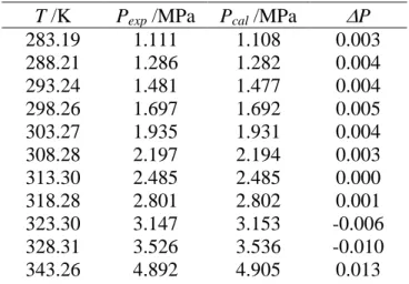
order to fit the Mathias Copeman coefficients: the Tillner – Roth’s (12) correlation for R32, and the Mc Linden’s (13) correlation for propane, from 248 K to critical temperatures of the corresponding component. The calculated values of the SRK EoS Mathias-Copeman coefficients are reported in Table 2. We have also measured the vapor pressures of the two pure components. Tables 3 and 4 (R32 and propane respectively)

report both our experimental data and pressures calculated with our model using the determined Mathias-Copeman coefficients. We have a good agreement between experimental and calculated vapour pressures showing good consistency between experimental data, literature correlations and our data treatment through the RKS EoS + Mathias-Copeman alpha function. The alpha functions are valid between 248 K and the critical temperatures of each component.

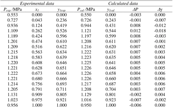
B) Vapor-liquid equilibrium: The VLE data obtained are listed in Tables 5 to 10. At each

temperature, we have adjusted the two (j,i and i,j) NRTL parameters. They appear slightly temperature dependent as shown in Figures 2 and 3.

Second order relationships are adequate for their representation:

12= 0.215T2 - 133.44T + 23579.72 (7)

 21= -0.139T2 + 77.35T - 8387.20 (8)

The results of modeling are reported in Tables 5 to 9 and plotted in Figure 4.

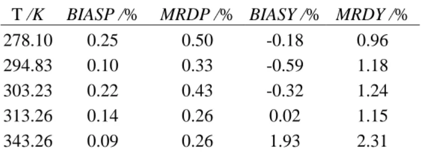
The mean relative absolute percentage deviations on pressure, MRDP, and the mean relative percentage deviations on vapor phase mole fraction, MRDY, listed in Table 10, are defined by:





_









 100/N U U_exp /U_exp

MRDU cal (9)

where U=P or y1 and N is the number of data points.

We have also calculated the BIAS values which are listed in table 10 and defined by eq (10):





_









BIASU _cal (10)

where U=P or y1 and N is the number of data points.

An accurate representation of the experimental data is found except at 343.26 K where adjustment and modeling is very difficult. At the mixture critical point the equation of state must calculate identical molar volumes for liquid and vapor phases. However, the SRK cubic equation of state is unable to calculate high-accuracy molar volumes close to the critical region. This may be the main reason for the modeling difficulty here.

C) PVT method: We have used another method to get results especially in the region

where a two phase-domain split was found and a poor representation was obtained. This was used to verify the data obtained from the static-analytic method. This second method selected here is the static-synthetic one with a variable volume cell. Herein, we measured only bubble pressures and compared them against the correlations. The uncertainties of the pressure is around 0.004 MPa and 0.1 K for the temperature. As displayed in Table 11, there is a good agreement (less than 1% for relative pressure deviation) between the two experimental methods. We have shown that left hand part of the diphasic envelope at 343.26 K really extends to xR32 about 0.5 while modeling stops at about 0.4. At this temperature there is clearly a modeling problem, not an experimental one. So we have changed the EoS and the mixing rules in order to have the best densities calculation. The Peng Robinson EoS (14) associated with the Wong-Sandler (15) mixing rules may well represent the last isotherm. The Wong-Sandler mixing rules are more adaptable with the third parameter kij, so in consequence all the densities are better calculated and the

experimental data are better represented specially at high pressure. The value of each parameters are given below and the isotherm is plotted on figure 5.

12= 1317,  21= 3135, k12=0.359.

D) Azeotrope line computation: An azeotrope corresponds to an extremum of temperature

or pressure. At this point the compositions of both liquid and vapor phases are equal. This can be expressed by,

0          P i x T for i=1 to N-1 (11) 0          T i x P for i=1 to N-1 (12) i i y x  for i=1 to N (13)

An azeotrope behaves like a pure fluid and then its components cannot be separated by simple distillation.

consequently, at equilibrium, EoS mixtures attractive parameters (a) at the azeotrope composition are the same in both the liquid and vapor phases. Conditions satisfying this equality allows computation azeotrope location. This method is suitable with an equation of state for isothermal or isobaric calculation.

Analytically, the advantage of this method is there are no derivatives to calculate. A simple secant method permits to obtain al=av at equilibrium where the compositions of the two phases are equal (x_i  y_i).

The computational algorithm is as follow: i) Input composition.

iii) Search for another composition where





 at equilibrium.

iv) Use the secant method to obtain third composition where av-al=0.

We show in the Table 12 and Figures 6 and 7 the characteristics of the azeotrope (pressure, temperature and composition). Equations (14) and (15) give the relation between T, Paz and xaz (R32).

Paz=379.61xaz2 – 451.39xaz + 134.13 (14)

Paz= 5.49810-4T2 - 0.275T + 35.26 (15) Note that the azeotropic composition of R32 increases with temperature.

E) Comparison with literature Data: Bobbo et al. (16) obtained data for this system at

lower temperatures but did not reproduce the liquid-liquid equilibrium mentioned by Holcomb et al. (16). We have fitted our model to their data. Then, we obtained two new parameters at each of their temperatures. Equations (16) and (17) represent the temperature dependence of the parameters obtained for each of our and Bobbo’s et al. temperatures, (248.15 to 343.26 K). Temperature dependence of parameters is continuous (see Figures 8 and 9) indicating consistency between the two data sets.

12= 0.189T2 – 111.73T + 19375 (16)

 21= -0.098T2 + 49.78T – 3817 (17)

The BIASU and MRDU were also calculated and the results are reported in Table 13. There’s a good agreement between experimental data and calculated data using the parameters 12 and 21 (Eqs (16) and (17)). Figure 10 gives the predictive curves along with experimental data (the 343.26 K isotherm does not appear in this figure).

F) Supercritical state: At 343.26 K, we have pointed out the disappearance of the phase

separation for xR32 between 0.5 and 0.85. The mixture becomes supercritical although the equilibrium temperature is lower than the critical temperature of the lightest component (R32). This isotherm and its two graphical critical end points are shown in Figure 4. An apparatus using the sapphire cell described by Laugier et al. (18) was used to observe the transition. At the critical point, a fog can be observed when the pressure is decreased. We can see in Figure 11 the different steps involving the fog and liquid formation. With this technique, we can record the pressure and the temperature for one composition after several increasing and decreasing of temperature. Two bubble pressures were measured and the results are given in Table 14. The precision for the pressure is 0.004 MPa and

0.1 K for the temperature. A correlating method to represent the critical point locus was established by Van Poolen and al. (19). Our critical data are congruent with the correlation, Figure 12 shows a plot indicating the VLE domain including the azeotrope line and the critical line from Van poolen et al..

Conclusion.

In this paper we present VLE data for the Propane+R32 system along several isotherm. Two experimental methods were used to verify the behaviour of this system. A static-analytic method and a PVT method were used to obtain the experimental data. The Soave-Redlich-Kwong (SRK EoS) equation of state, with a Mathias-Copeman alpha function and MHV1 mixing rules was chosen to conveniently fit VLE data except for the critical isotherm at 343.26 K where the Peng Robinson (PR EoS) and the Wong Sandler isotherm were used. At this temperature, there are two critical points. The azeotrope location is given as a function of temperature (see Figure 11).

List of symbols

a Parameter of the equation of state (attractive parameter)

b Parameter of the equation of state (co volume parameter)

G Gibbs free energy

F Objective function

P Pressure [MPa]

R Gas constant [J.mol-1 K-1]

T Temperature [K]

Z Compressibility factor

x Liquid mole fraction

y Vapor mole fraction N Number of component Greek letters

ij NRTL model parameter (eq 5)

ij NRTL model binary interaction parameter (eq 5) [J.mol-1]

 Acentric factor  Deviation Superscript E Excess property Subscripts C Critical property cal Calculated property exp Experimental property i,j Molecular species

az Azeotrope

v Vapor phase

l liquid phase

1 R32

References :

(1) Montreal Protocol on substances that deplete the ozone layer, United Nations Environmental Program (UNEP), Final Act, United Nations, New York, NY, USA, 1987. (2) Laugier, S.; Richon, D. New apparatus to perform fast determinations of mixture vapor – liquid equilibria up to 10 MPa and 423 K. Rev. Sci. Instrum. 1986, 57, 469-472. (3) Fontalba, F.; Richon, D.; Renon, H. Simultaneous determination of vapour liquid equilibria and volumetric properties up to 45 MPa and 160°C by the static method using a variable volume cell without sampling. CR Acad.Sci.Paris, 1982, 2, 944-951.

(4) Valtz, A.; Laugier, S.; Richon, D.; Bubble pressures and saturated liquid molar volumes of difluoromonochloromethane-fluorochloroethane binary mixtures: experimental data and modeling. Int. J. Refrig. 1986, 9, 282-289.

(5) Guilbot, P.; Valtz, A.; Legendre, H.; Richon D. Rapid On Line Sampler-Injector, a reliable tool for HT-HP Sampling and on line GC analysis. analusis 2000, 28, 426-431. (6) Huber, M.; Gallagher, J.; McLinden, M. O.; Morrison, G. Thermodynamic Properties of Refrigerants and Refrigerant Mixtures Database. REFPROP V.6.01. National Institute of Standards and Technology. Gaithersburg, MD, 1996.

(7) 17th IUPAC Conference on Chemicals Thermodynamics, Rostok July 28 August 02, 2002.

(8) Soave, G. Equilibrium constants for modified Redlich-Kwong equation of state.

Chem. Eng. Sci. 1972, 4, 1197-1203.

(9) Mathias, P. M. and Copeman, T. W. Extension of the Peng-Robinson Equation of State to Complex Mixtures: Evaluation of Various Forms of the Local Composition Concept. Fluid Phase Equilib. 1983, 13, 91-108.

(10) Michelsen, M. A modified HURON-VIDAL mixing rule for cubic equations of state.

Fluid Phase Equilib. 1990, 60, 213-219.

(11) Renon, H. and Prausnitz, J.M., Local Composition in Thermodynamic Excess Function for Liquid Mixtures. AIChE J. 1968, 14, 135-144.

(12) Tillner-Roth, R.; Yokozeki, A. An international standard equation of state for difluoromethane (R32) for temperatures from triple point at 136.34 K to 435 K and pressures up to 70 MPa. J.Phys.Ref.Data 1997, 26, 1273-1328.

(13) McLinden, M.O. Thermodynamic properties of CFC alternatives: a survey of the available data. Rev. Int. Froid. 1990, 13, 149-162.

(14) Peng, D. Y., Robinson, D. B.,A new two parameters Equation of State. Ind. Eng.

(15) Wong, D. S. H., Sandler S. I., A Theoretically Correct Mixing Rules for Cubic Equation of State. AIChE. 1992, 38, 671-680.

(16) Bobbo, S.; Fedele, L.; Camporese, R.; Stryjek R. VLE measurements and modeling for the strongly positive azeotropic R32 + propane system. Fluid Phase Equilib. 2002,

199, 175-183.

(17) Holcomb, C.D.; Magee, J.W.; Scott, J.R.; Outcalt, S.L.; Haynes, W.M. NIST Technical Note 1397. NIST: Gaithersburg, December 1997.

(18) Laugier, S.; Richon, D.; Renon, H. Simultaneous determination of vapor-liquid equilibria and volumetric properties of ternary systems with a new experimental apparatus. Fluid Phase Equilib. 1990, 54, 19-34.

(19) Van Poolen, L.J.; Holcomb, C.D.; Rainwater, J.C. Isoplethic method to Estimate Critical lines for Binary Fluid Mixtures from Subcritical Vapor-Liquid Equilibrium: Application to the Azeotropic Mitures R32 + C3H8 and R125 + C3H8. Ind. Eng. Chem.

Table 1. Critical Parameters and acentric Factors from REFPROP (3)

Compound Pc /MPa Tc /K  Propane 4.246 369.95 0.152

Table 2. Ajusted Mathias-Copeman Coefficients

Coefficients R32 Propane

C1 1.034 0.789

C2 -1.454 -0.894

Table 3. Experimental and calculated vapor pressures of R32 (SRK EoS)

T /K Pexp /MPa Pcal /MPa P 283.19 1.111 1.108 0.003 288.21 1.286 1.282 0.004 293.24 1.481 1.477 0.004 298.26 1.697 1.692 0.005 303.27 1.935 1.931 0.004 308.28 2.197 2.194 0.003 313.30 2.485 2.485 0.000 318.28 2.801 2.802 0.001 323.30 3.147 3.153 -0.006 328.31 3.526 3.536 -0.010 343.26 4.892 4.905 0.013

Table 4. Experimental and calculated vapor pressures of Propane (SRK EoS) T /) Pexp /MPa Pcal /MPa P

277.17 0.536 0.535 0.001 283.22 0.638 0.638 0.000 288.26 0.734 0.734 0.000 293.27 0.838 0.839 0.001 298.30 0.955 0.955 0.000 302.27 1.055 1.055 0.000 308.80 1.236 1.236 0.000 311.80 1.326 1.326 0.000 313.24 1.370 1.371 -0.001 318.22 1.537 1.536 0.001 323.22 1.716 1.715 0.001 328.26 1.911 1.911 0.000 333.29 2.120 2.122 -0.002 338.31 2.346 2.350 -0.004 343.26 2.591 2.593 -0.002 348.31 2.852 2.859 -0.007 353.41 3.134 3.149 -0.014

Table 5. Vapor-liquid Equilibrium Pressures and Phase Compositions for R32 (1) + Propane (2) Mixtures at 278.10 K

Experimental data Calculated data

Pexp /MPa x1 y1exp Pcal /MPa y1cal P y

0.553 0.000 0.000 0.550 0.000 -0.003 0.000 0.727 0.043 0.236 0.726 0.243 -0.001 -0.007 0.936 0.124 0.419 0.944 0.431 0.008 -0.012 1.109 0.262 0.526 1.121 0.544 0.012 -0.018 1.189 0.424 0.596 1.197 0.599 0.008 -0.003 1.201 0.474 0.610 1.208 0.611 0.007 -0.001 1.209 0.516 0.622 1.216 0.620 0.007 0.002 1.215 0.563 0.634 1.222 0.631 0.007 0.003 1.218 0.583 0.639 1.223 0.635 0.005 0.004 1.220 0.608 0.646 1.225 0.641 0.005 0.005 1.221 0.628 0.651 1.226 0.646 0.005 0.005 1.222 0.673 0.664 1.226 0.658 0.004 0.006 1.221 0.680 0.666 1.226 0.660 0.005 0.006 1.214 0.756 0.693 1.217 0.687 0.003 0.006 1.205 0.791 0.711 1.208 0.704 0.003 0.007 1.131 0.909 0.805 1.129 0.801 -0.002 0.004 1.023 0.975 0.921 1.016 0.923 -0.007 -0.002 0.956 1.000 1.000 0.950 1.000 -0.006 0.000

Table 6. Vapor-liquid Equilibrium Pressures and Phase Compositions for R32 (1) + Propane (2) Mixtures at 294.83 K

Experimental data Calculated data

Pexp /MPa x1 y1exp Pcal /MPa y1cal P y

0.874 0.000 0.000 0.874 0.000 0.000 0.000 0.926 0.008 0.049 0.922 0.050 -0.004 -0.001 1.123 0.046 0.206 1.121 0.216 -0.002 -0.010 1.206 0.064 0.261 1.202 0.269 -0.004 -0.008 1.406 0.123 0.370 1.413 0.385 0.007 -0.015 1.693 0.264 0.508 1.699 0.511 0.006 -0.003 1.840 0.439 0.584 1.851 0.586 0.011 -0.002 1.897 0.599 0.645 1.908 0.641 0.011 0.004 1.900 0.618 0.650 1.911 0.648 0.011 0.002 1.906 0.694 0.684 1.913 0.678 0.007 0.006 1.903 0.731 0.699 1.908 0.695 0.005 0.004 1.897 0.759 0.713 1.900 0.709 0.003 0.004 1.880 0.802 0.746 1.881 0.735 0.001 0.011 1.715 0.941 0.877 1.710 0.875 -0.005 0.002 1.677 0.957 0.903 1.672 0.903 -0.005 0.000 1.547 1.000 1.000 1.542 1.000 -0.005 0.000

Table 7. Vapor-liquid Equilibrium Pressures and Phase Compositions for R32 (1) + Propane (2) Mixtures at 303.23 K

Experimental data Calculated data

Pexp /MPa x1 y1exp Pcal /MPa y1cal P y

1.255 0.027 0.126 1.253 0.130 -0.002 -0.004 1.492 0.073 0.258 1.495 0.270 0.003 -0.012 1.824 0.165 0.404 1.833 0.413 0.009 -0.009 2.076 0.287 0.503 2.090 0.506 0.014 -0.003 2.262 0.456 0.590 2.272 0.583 0.010 0.007 2.311 0.535 0.615 2.320 0.615 0.009 0.000 2.317 0.564 0.630 2.332 0.626 0.015 0.004 2.336 0.646 0.665 2.352 0.661 0.016 0.004 2.340 0.694 0.689 2.353 0.684 0.013 0.005 2.345 0.705 0.695 2.352 0.689 0.007 0.006 2.318 0.794 0.747 2.320 0.740 0.002 0.007 2.226 0.890 0.824 2.218 0.821 -0.008 0.003 2.094 0.953 0.916 2.084 0.905 -0.010 0.011 1.937 1.000 1.000 1.929 1.000 -0.008 0.000

Table 8. Vapor-liquid Equilibrium Pressures and Phase Compositions for R32 (1) + Propane (2) Mixtures at 313.26 K

Experimental data Calculated data

Pexp /MPa x1 y1exp Pcal /MPa y1cal P y

1.496 0.017 0.075 1.497 0.077 0.001 -0.002 1.608 0.034 0.133 1.613 0.138 0.005 -0.005 2.344 0.198 0.412 2.363 0.417 0.019 -0.005 2.540 0.272 0.475 2.555 0.472 0.015 0.003 2.720 0.367 0.530 2.730 0.526 0.010 0.004 2.844 0.468 0.583 2.859 0.575 0.015 0.008 2.931 0.582 0.639 2.949 0.631 0.018 0.008 2.940 0.605 0.649 2.960 0.642 0.020 0.007 2.952 0.622 0.658 2.966 0.651 0.014 0.007 2.964 0.710 0.705 2.975 0.699 0.011 0.006 2.923 0.799 0.761 2.934 0.756 0.011 0.005 2.880 0.844 0.797 2.887 0.792 0.007 0.005 2.685 0.947 0.901 2.677 0.906 -0.008 -0.005 2.491 1.000 1.000 2.483 1.000 -0.008 0.000

Table 9. Vapor-liquid Equilibrium Pressures and Phase Compositions for R32 (1) + Propane (2) Mixtures at 343.26 K

Experimental data Calculated data

Pexp /MPa x1 y1exp Pcal /MPa y1cal P y

2.591 0.000 0.000 2.593 0.000 0.002 0.000 3.139 0.065 0.146 3.165 0.148 0.026 -0.002 3.499 0.113 0.226 3.519 0.220 0.020 0.006 3.964 0.188 0.310 3.977 0.297 0.013 0.013 4.222 0.237 0.345 4.225 0.333 0.003 0.012 4.442 0.282 0.375 4.423 0.360 -0.019 0.015 4.702 0.345 0.420 4.658 0.388 -0.044 0.032 5.009 0.432 0.472 5.003 0.432 -0.006 0.040 5.077 0.457 0.480 5.075 0.457 -0.002 0.023 5.451 0.858 0.849 5.451 0.858 0.000 -0.009 5.413 0.876 0.866 5.415 0.873 0.002 -0.007 5.308 0.911 0.901 5.313 0.900 0.005 0.001 5.259 0.924 0.915 5.267 0.912 0.008 0.003 5.201 0.939 0.930 5.208 0.927 0.007 0.003 5.049 0.972 0.965 5.058 0.964 0.009 0.001 4.940 0.992 0.989 4.951 0.989 0.011 0.000 4.892 1.000 1.000 4.905 1.000 0.013 0.000

Table 10. Mean Relative Absolute Deviations in Pressure, MRDP, Vapor Phase Compositions, MRDY, and Bias using the Soave-Redlich-Kwong Equation of State with MHV1 Mixing Rules

T /K BIASP /% MRDP /% BIASY /% MRDY /%

278.10 0.25 0.50 -0.18 0.96

294.83 0.10 0.33 -0.59 1.18

303.23 0.22 0.43 -0.32 1.24

313.26 0.14 0.26 0.02 1.15

Table 11. Bubble Point Data Measured by the PVT method and Calculated by SRK + MHV1 + NRTL Models

T /K Pexp /MPa x1 Pcal /MPa y1cal P

287.53 1.533 0.439 1.542 0.593 -0.009 323.25 3.455 0.439 3.482 0.542 -0.027 333.04 4.186 0.439 4.207 0.509 -0.021 343.10 3.876 0.173 3.884 0.284 -0.008 343.18 4.821 0.388 4.780 0.388 0.041 333.49 4.090 0.388 4.109 0.477 -0.019 342.15 4.874 0.406 4.823 0.406 0.051 333.49 4.129 0.406 4.156 0.487 -0.027 295.38 1.869 0.465 1.890 0.594 -0.021 303.67 2.278 0.465 2.302 0.586 -0.024 313.02 2.817 0.465 2.841 0.574 -0.024 323.35 3.497 0.465 3.532 0.556 -0.035 333.17 4.251 0.465 4.278 0.524 -0.027 337.85 4.629 0.465 4.641 0.493 -0.012 340.42 4.739 0.465 4.698 0.465 0.041 332.75 4.404 0.866 4.391 0.838 0.013 323.16 3.572 0.866 3.570 0.824 0.002

Table 12. Composition and Pressure of the Azeotrope (R32) at Each Temperature (MHV1 Mixing Rules)

T /K xaz exp Pexp /MPa xaz cal Pcal /MPa P x

278.10 0.663 1.221 0.653 1.226 -0.005 0.010 294.83 0.679 1.906 0.666 1.914 -0.008 0.023 303.23 0.683 2.342 0.674 2.354 -0.012 0.009 313.26 0.702 2.961 0.684 2.977 -0.016 0.018 323.00 0.694 3.699 333.00 0.705 4.580

Table 13. Mean Relative Absolute Deviations in Pressure, MRDP, Vapor Phase Composition, MRDY, and Bias using the Soave-Redlich-Kwong Equation of State with MHV1 Mixing Rules

T /K BIASP /% MRDP /% BIASY /% MRDY /%

Bobbo and al 248.15 -0.18 0.26 0.46 0.63 254.15 -0.11 0.45 -0.03 0.74 273.15 -0.05 0.41 1.20 1.21 294.91 -0.08 0.36 0.96 1.05 This work 278.10 0.39 0.42 -0.09 0.74 294.83 0.37 0.38 -0.25 0.79 303.23 0.27 0.33 0.03 0.19 313.26 0.12 0.16 0.29 0.75 343.26 0.12 0.25 2.60 2.91

Table 14. Critical Points Measured by the PVT Equipment with a Sapphire Variable Volume Cell

T /K P /MPa xR32 342.50 5.210 0.527 344.00 5.532 0.866

Figure 1. Flow diagram of the equipment:

C: Carrier Gas; EC: Equilibrium Cell; FV: Feeding Valve; LB: Liquid Bath; PP: Platinum Probe; PrC: Propane Cylinder; PT: Pressure Transducer; RC: Refrigerant Cylinder; SM: Sampler Monitoring; SW: Sapphire window; TC1 and TC2 Thermal Compressors; Th: Thermocouple; TR: Temperature Regulator; VSS: Variable Speed Stirring; VP: Vacuum Pump. TR PT SM VP PrC RC TR TR TC1 TC2 PP PP VSS Th TR C SW TR LB

Figure 2.  NRTL Binary parameter as a function of temperature: ♦; fitted to isotherm ; __; eq (7).

Figure 3.  NRTL Binary parameter as a function of temperature: ♦; fitted to isotherm; __; eq (8).

Figure 4. VLE for the R32 (1) + propane (2) system at different temperatures: ●; 278.10 K; ▲; 294.83 K; *; 303.23 K; ; 313.26 K ; ■; 343.26 K;

+; graphical end points;

solid lines, calculated with RKS EoS and MHV1 mixing rules ; dashes lines ---, calculated at 323 K;

dashes lines _ _ _, calculated at 333 K ; ♦; Azeotrope location. 0 1 2 3 4 5 6 0.0 0.2 0.4 0.6 0.8 1.0 x1, y1 P / M Pa

Figure 5. VLE for the R32 (1) + propane (2) system at 343.26 K. solid lines, calculated with PR EoS and Wong Sandler mixing rules ;

2.5 3.0 3.5 4.0 4.5 5.0 5.5 0.0 0.2 0.4 0.6 0.8 1.0 x1, y1 P / M Pa

Figure 6. Azeotropic composition (R32) as function of temperature. ♦; calculated azeotrope ; __ ; eq (14). 0.65 0.66 0.67 0.68 0.69 0.70 0.71 275 285 295 305 315 325 335 345 T / K A z e o tr o p e c o m p o si ti o n

Figure 7. Azeotropic pressure as function of temperature. ♦ ; calculated azeotrope ; __; eq (15). 0.5 1.0 1.5 2.0 2.5 3.0 3.5 4.0 4.5 5.0 275 285 295 305 315 325 335 345 T / K Paz / M Pa

Figure 8.  NRTL Binary parameter as function of temperature: ▲; from Bobbo et al.; ▪; this work ; __; eq (16).

Figure 9.  NRTL Binary parameter as function of temperature: ▲; from Bobbo et al.; ▪ ; this work ; __; eq (17).

Figure 10. VLE for the R32 (1) + propane (2) system at all different temperatures with experimental data. 0.1 0.5 0.9 1.3 1.7 2.1 2.5 2.9 0.0 0.2 0.4 0.6 0.8 1.0 Composition x1, y1 P re s s u re / M P a

Figure 12. P,T diagram of the R32-propane system: ---; Critical locus from Van Poolen et al.;

; Critical point measured by the PVT (Sapphire cell); ♦; Azeotrope calculation. 0.5 1.0 1.5 2.0 2.5 3.0 3.5 4.0 4.5 5.0 5.5 6.0 270 290 310 330 350 370 390 T /K P / M Pa Propane R32 Azeotrope

1) 2) 3) Figure 11. The different steps to characterize a mixture critical point: 1) mixture in supercritical state;

2) The pressure decreases (beginning of fog formation); 3) The fog leads to a liquid phase.

Fog Sapphire

cell