PM2.5 low-cost sensor perfomance in ambient conditions

PM2.5 low-cost sensor performance in ambient conditions

C. Falzone

_{, A.-C. Romain}

_{, S. Guichaux}

_{, V. Broun}

_{, D. Rüffer}

_{, G. Gérard}

_{, F.}

Lenartz

1. Introduction

The use of low-cost air quality sensors to evaluate personal exposure, complement a monitoring network or perform real-time data assimilation is spreading. Although some laboratories and project consortiums have set up their own procedures to assess the performan ce of such systems [1, 2] and although the CEN TC264 WG42 is preparing two standards on that topic, so far the only European reference remains the Guidance for the Demonstration of Equivalence of Ambient Air Monitoring Methods [3] that holds for any

This short paper presents the application on a recent data set of some generic statistical tests and the demonstration of equivalence to evaluate the performance of various air quality nodes. The demonstration of equivalence uses an orthogonal regression whereas a majority of papers present a linear model based on total least square [4, 5]. In Section 2, we present the measurement campaign set up, the devices and their main characteristics, as well as the metrics used to assess their performance. In Section 3, we show and discuss the results, whereas in Section 4, we draw our conclusion.

2. Material and methods

In this study, six devices based on low-cost sensors and designed by three different institutions are compared during three measurement campaigns held in January, February and April 2020. Their reliability is simply estimated in terms of data coverage, while their metrological performance is assessed on one hand by a comparison of statistical test results, error metrics and method agreement analysis, on the other hand by following, as closely as possible, the methodology for the demonstration of equivalence known and used by monitoring network managers.

2.1. Campaign

The measurement campaign set up for this study is an add-on to the one led annually by the Air Quality Department of ISSeP to verify and/or update the calibration factors of their PMX monitors. In this work,

three sites are investigated, the urban background station of Herstal from January 25th _{to February 6}th_{, the}

suburban background station of Angleur from February 8th _{to February 20}th _{and the temporary traffic station}

1_{SAM ULiège, Arlon (Belgium), [email protected]} 2_{CECOTEPE, Seraing (Belgium)}

3_{Sensirion AG, Stäfa (Switzerland)} 4_{ISSeP, Liège (Belgium)}

of Charleroi from April 10th _{to April 22}nd_{. This last site is investigated during the Belgian lockdown due to}

COVID19.

2.2. Measurement systems

The sampler used for the reference gravimetric method is a conditioned Derenda PNS 16-6.1, while the instrument used as the equivalent method is the Grimm EDM180. The calibration equation in use since 2010 for PM2.5 is . Nevertheless, for our tests we decide to consider the Grimm like the

other devices and use the raw data. Gravimetric data are only available for the sites of Angleur and Charleroi, because a PM10 head was used in Herstal.

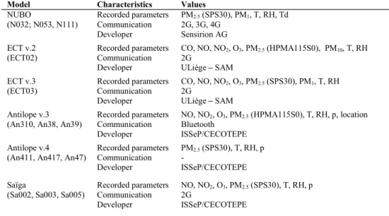
One commercial and five non-commercial systems based on low-cost commercial sensors are tested: the Nubo from Sensirion AG (3 replicates), the EcoCityTool v.2 (1) and v.3 (1) from ULiège and the Antilope v.3 (3) and 4 (3) as well as the Saiga (3) from ISSeP/CECOTEPE. Their main characteristics are reported in Table 1. All these automatic mini-stations are based either on the Honeywell HPMA115S0 or on the Sensirion SPS30 sensors for PM2.5. The principle of measurement, light-scattering, is similar for

both but they differ in the way they estimate mass concentration based on count concentration. The Grimm is also based on light-scattering but has a larger range and discriminate 32 particle sizes.

Model Characteristics Values

NUBO Recorded parameters PM2.5 (SPS30), PM1, T, RH, Td

(N032; N053, N111) Communication 2G, 3G, 4G

Developer Sensirion AG

ECT v.2 Recorded parameters CO, NO, NO2, O3, PM2.5 (HPMA115S0), PM10, T, RH

(ECT02) Communication 2G

Developer ULiège SAM

ECT v.3 Recorded parameters CO, NO, NO2, O3, PM2.5 (SPS30), PM1, T, RH

(ECT03) Communication 2G

Developer ULiège SAM

Antilope v.3 Recorded parameters NO, NO2, O3, PM2.5 (HPMA115S0), T, RH, p, location

(An310, An38, An39) Communication Bluetooth

Developer ISSeP/CECOTEPE

Antilope v.4 Recorded parameters PM2.5 (SPS30), T, RH, p

(An411, An417, An47) Communication -

Developer ISSeP/CECOTEPE

Saïga Recorded parameters NO, NO2, O3, PM2.5 (SPS30), T, RH, p

(Sa002, Sa003, Sa005) Communication 2G

Developer ISSeP/CECOTEPE

Table 1. Automatic mini- .

2.3. Performance evaluation

Square Error (RMSE). Both error metrics provide a value in the same units as the original signals, the latter

g a Bland-Altman analysis. Finally, the verification of equivalence is done based on a limit value of 25 µg/m³, the relative expended uncertainty (WCM) is set to 25% (uncertainty for fixed measurements according to the 2008/50/EC directive; it is set to

50% for indicative measurements) and the reference squared uncertainty equals 0.2221 (µg/m³)². Depending on the results, a calibration will be required for some devices to reach the data quality objective. All data analyses are performed with R and the following libraries: openair, blandr, DescTools and Metrics.

3. Results

All low-cost measurements presented here have a 1-minute interval. When compared to the Grimm they are averaged with a 30-minute interval and when compared to the gravimetric method with a 1-day interval. For these aggregations a 75% capture rate is required, otherwise the value is considered as not available.

3.1. Preliminary tests

As a first step, we check data availability and discard instruments for which the coverage rate is less than 75% in each period (see Table 2).

Herstal Angleur Charleroi

n % [min-max] n % [min-max] n % [min-max] n total % total An310 19067 100 [0-93.5] 18735 100 [0.3-45.4] 18747 100 [3.2-58.4] 56549 100% An38 19067 100 [0-97.7] 18735 100 [0.2-43.3] 18747 100 [2.7-61.8] 56549 100% An39 19066 100 [0-194.6] 0 0 - 18747 100 [1.9-119.4] 37813 67% An411 0 0 - 18699 100 [0-31.2] 0 0 - 18699 33% An417 19030 100 [0-103] 0 0 - 18710 100 [0.8-68.4] 37740 67% An47 0 0 - 18699 100 [0-29.4] 18710 100 [0.7-73.5] 37409 66% Sa002 10747 56 [0.3-53.3] 13110 70 [0.7-31] 4702 25 [2-19.6] 28559 51% Sa003 13730 72 [0.2-46.7] 10575 56 [0.6-24.3] 18165 97 [1-57.5] 42470 75% Sa005 16785 88 [0-98.8] 17830 95 [0.5-21.2] 18174 97 [1.3-60.1] 52789 93% N032 18801 99 [0.1-111.6] 18434 98 [0.2-29.9] 18535 99 [1.7-58.6] 55770 99% N053 18758 98 [0.1-106.2] 18293 98 [0.2-25.8] 18408 98 [1.7-55.7] 55459 98% N111 18764 98 [01-109.6] 18557 99 [0.3-32.5] 18594 99 [1.7-54.8] 55915 99% ECT02 14525 76 [0-75] 18457 99 [0-26] 13620 73 [1-155] 46602 82% ECT03 19067 100 [0-79.1] 18735 100 [0.2-46.4] 0 0 - 37802 67%

Table 2. Number of data, coverage percentage and minimal and maximal values collected during each campaign and for all of them.

As a second step, we make a visual inspection of the time series and a summary of the distribution via boxplot and whiskers.

Fig. 1. Time series of the 14 instruments tested along the reference and equivalent methods. The red line is the median of the ensemble of instruments, the grey ribbon represents its interquartile range and the

lightblue line the An39 device.

As can be seen in Figure 1, all sensors display a similar behavior over time for each period, except for the An39 (lightblue). However, the amplitude of the signals varies slightly from one sensor to the others as can be seen in Table 1. The levels observed in Herstal are below 20 µg/m3 _{except during the first two and}

last two days, where they reach up to 50 µg/m3_{. In Angleur, concentrations remain low (< 15 µg/m}3_{) during}

the whole campaign. For both these periods we have measured an amount of about 50 mm of precipitation, while the average wind speed was slightly higher for the second period than for the first, with respectively 4.79 m/s and 3.23 m/s. During the last period in Charleroi, a more diverse profile of concentrations is observed, e.g. a narrow peak on April 13th _{night, some days with an increase during the night and a decrease}

in the late morning, a whole day with PM2.5 concentrations higher than 20 µg/m3 on April 19th.

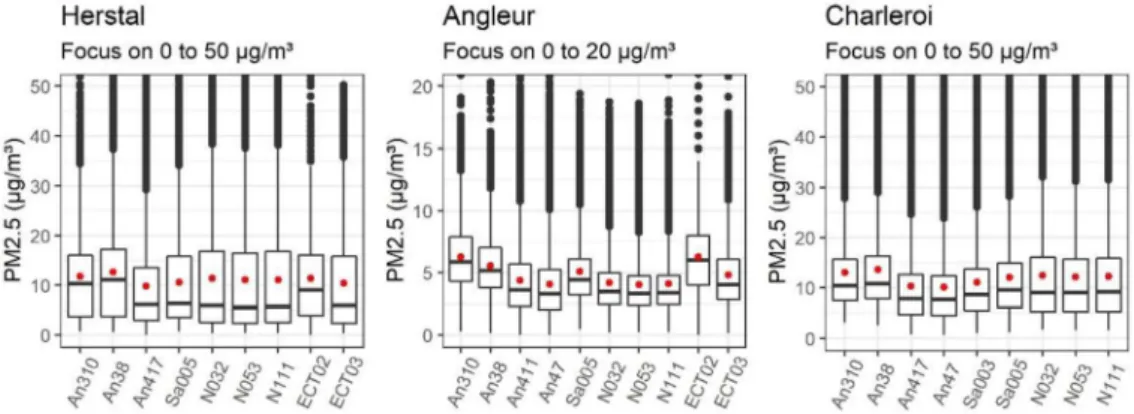
In Figure 2, one can clearly see the dependence of the distribution on the sensor model, at least for the first two boxplots. Both in Herstal and Angleur, the An310, An38 and ECT02, all equipped with a HPMA115S0, present a median higher than the one displayed by the devices with the SPS30 and also closer to their mean. The inter-quartile ranges are very similar in each device family.

Fig. 2. Boxplots of the different devices for which the coverage rate is greater than 75% in each period and for a common period between devices. The red dot corresponds to the mean.

3.2. Statistical tests, error metrics and equivalence

The statistics tests are in accordance to the boxplots shown in Figure 2. The Kruskal-Wallis test applied on the ensemble of devices for each period presents a p-value < 0.05, hence the H0

-Whitney-Wilcoxon tests present a

p-mostly those with the same SPS30 sensor (Herstal: An417 with the 3 Nubo and ECT03, ECT03 with the 3 Nubo and the 3 Nubo with each other; Angleur: An310 with ECT02; Charleroi: An417 with An47 and the 3 Nubo with each other).

The equivalence demonstration is done for Angleur and Charleroi. The common periods, for which the capture rate of the devices is higher than 75%, includes respectively 11 and 13 days.

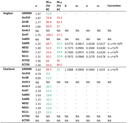
For Angleur, only the Grimm with a WCM = 11. 9% passes directly the equivalence test, the other

sensors need to be calibrated. Thereafter, four additional devices sensors pass the test, namely the Sa005 with a WCM = 22.2% (68.7% before calibration), the N032 with a WCM = 24.4%

(52.5% before calibration), the N053 with a WCM = 23.4% (53.6% before calibration) and the

N111 with a WCM = 22.8% (50.1% before calibration). All these devices were built with an

SPS30 sensor.

For Charleroi, only the Grimm fails the equivalence test and needs a calibration to pass with a WCM = 22% (66.5% before calibration). Devices based on both the Honeywell and the Sensirion

sensors pass directly the test.

Table 3 summarizes the results of the demonstration of equivalence, including calibration equation. In order to complete the analysis, one can mention that the average and the standard deviation of the reference method in Angleur are 5.46 µg/m3 _{and 3.47 µg/m}3_{, and in Charleroi 13.08 µg/m}3 _{and 6.45 µg/m}3_.

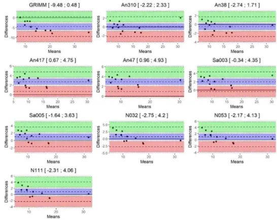
In addition, a Bland-Altman plot [5] is drawn for each device in respect with the reference method (see F

closely as possible to 0 for the whole range of observed values. The bias corresponds to the mean error. The limits of agreement correspond to 1.96 times the standard deviation of the differences against the bias. For the measurement campaign in Charleroi, one can see in the upper left corner subplot that the bias of the Grimm is far from 0 with a value of -4.5 µg/m3_{, that the repeatability (half the distance between the limits}

of agreement) is high with a value of 9.96 µg/m3 _{and that a tendency of increasing gaps with increasing}

values is displayed; all these elements make the instrument, a priori, a not so good candidate for the equivalence. Nevertheless, the impact of calibration is also directly visible on the Bland-Altman plot, as shown in Figure 4. The limits of agreement are widely reduced and the bias is nearly equal to 0; the rmined in 2010, the repeatability decreases from 4.98 µg/m3 _{to 2.97 µg/m}3 _{and the Grimm fails the test of equivalence}

(27.5%).

Table 3. Demonstration of equivalence for Angleur and Charleroi. Devices that pass the test are in green,

u W CM (%) BC WCM (%) AC b ub a ua Correction Angleur GRIMM 1.37 11.9 - - - - An310 1.87 74.8 76.4 An38 1.77 89.4 82.3 An411 1.66 99.9 27 An417 NA NA NA NA NA NA NA NA An47 1.75 100.5 27.5 Sa003 NA NA NA NA NA NA NA NA

Sa005 1.22 68.7 22.2 0.5772 0.0817 2.0228 0.5217 yi.cal=(yi-a)/b

N032 1.30 52.5 24.4 0.7275 0.0992 0.3300 0.6330 yi.cal=yi/b

N053 1.37 53.6 23.4 0.7283 0.0975 0.1705 0.6220 yi.cal=yi/b

N111 1.31 50.1 22.8 0.7472 0.0968 0.1270 0.6178 yi.cal=yi/b

ECT02 1.56 64 36

ECT03 1.34 59.4 40.5

Charleroi GRIMM 3.62 66.5 22 1.2988 0.0909 0.5964 1.3155 yi.cal=yi/b

An310 0.79 9.4 - - - - An38 0.85 11.5 - - - - An411 NA NA NA NA NA NA NA NA An417 2.04 20.7 - - - - An47 2.19 23.5 - - - - Sa003 1.63 19.8 - - - - Sa005 1.15 10.2 - - - - N032 1.31 16.2 - - - - N053 1.29 12.6 - - - - N111 _{1.27 13.2} - - - - ECT02 NA NA NA NA NA NA NA NA ECT03 NA NA NA NA NA NA NA NA

Fig. 3. Bland-Altman plots for the measurement campaign in Charleroi. The intermediate dashed line represents the bias between the method, both others the upper and the lower limit of agreement (their value is also in the title of each subplot). The green ribbon corresponds to the IC 95% on the upper L.A.,

-Fig. 4. Bland-Altman plots before (left) and after (right) calibration and the regression plot (middle) for the Grimm in Charleroi.

Bland-From our two

correlated, meaning that a good rank correlation does not necessarily lead to a good concordance correlation and conversely, e.g. Grimm in Charleroi. According to a subjective classification in the literature [7], all -0.95], respectively) pass directly the equivalence -0.6]; [0.61-0.7], respectively) always fail the test even -0.8]; [0.81-0.9], respectively) labels does not allow one to conclude anything.

As well, one cannot draw any conclusion based on both chosen error metrics. They usually depend too much on the concentration levels observed; they may be useful in relative terms but it has not been tested here.

L.A. lower

L.A.

upper Bias Accuracy Repeat. Slope Spearman Lin MAE RMSE GRIMM -4.05 1.09 -1.48 1.76 2.57 0.13 0.73 0.82 Fairly good 1.75 1.93

An310 -6.01 4.23 -0.89 2.4 5.12 0.59 0.71 0.55 Poor 2.40 2.64 An38 -5.33 4.95 -0.19 2.07 5.14 0.7 0.71 0.55 Poor 2.06 2.50 An411 -3.37 5.36 0.99 1.52 4.36 0.8 0.72 0.61 Mediocre 1.52 2.34 An417 - - - - An47 -3 5.63 1.31 1.68 4.31 0.77 0.63 0.59 Poor 1.68 2.47 Sa003 - - - -

Sa005 -3.2 3.77 0.28 1.18 3.48 0.52 0.86 0.80 Fairly good 1.18 1.71 N032 -1.8 4.11 1.15 1.26 2.95 0.3 0.82 0.81 Fairly good 1.26 1.84 N053 -1.61 4.23 1.31 1.34 2.92 0.3 0.86 0.80 Fairly good 1.34 1.93 N111 -1.56 4.07 1.25 1.28 2.81 0.28 0.86 0.81 Fairly good 1.27 1.85 ECT02 -5.04 3.24 -0.9 2.04 4.14 0.54 0.71 0.69 Mediocre 2.04 2.20 ECT03 -3.18 4.27 0.54 1.38 3.72 0.39 0.63 0.78 Satisfactory 1.37 1.89 GRIMM -9.48 0.48 -4.5 4.52 4.98 -0.26 0.95 0.78 Satisfactory 4.52 5.12 An310 -2.22 2.33 0.05 0.94 2.27 0.03 0.93 0.98 Excellent 0.94 1.11 An38 -2.7 1.71 -0.49 0.96 2.20 -0.03 0.94 0.98 Excellent 0.95 1.20 An411 - - - -

An417 0.67 4.75 2.71 2.71 2.04 -0.02 0.93 0.90 Very good 2.71 2.88

An47 0.96 4.93 2.94 2.94 1.98 -0.01 0.95 0.88 Fairly good 2.94 3.09

Sa003 -0.34 4.35 2.00 2 2.34 0.01 0.94 0.93 Very good 2.00 2.31

Sa005 -1.64 3.63 0.99 1.43 2.63 -0.07 0.95 0.96 Excellent 1.42 1.63 N032 -2.75 4.2 0.72 1.54 3.47 -0.16 0.93 0.96 Excellent 1.54 1.85 N053 -2.17 4.13 0.98 1.5 3.15 -0.12 0.93 0.96 Excellent 1.49 1.83 N111 -2.31 4.06 0.87 1.5 3.18 -0.13 0.93 0.96 Excellent 1.46 1.78 ECT02 - - - - ECT03 - - - -

Table 4. Limits of agreement (L.A.), bias, accuracy, coefficient of repeatability and slope of the

Bland-Absolute Error and Root-Mean-Square Error for Angleur (above) and Charleroi (below). Devices that pass the equivalence test directly are in green, devices that pass it after calibration in orange and devices

that fail it in red.

noticing that only two sites are investigated, that the range of measured values is relatively limited and that a rather short period of the year is covered.

All these parameters are performance indicators and could be used as-is or in combination to evaluate the metrological quality of a device. However, to find an alternative to the demonstration of equivalence without adding some subjective or site-dependent thresholds seems, on the mere basis of these two measurement campaigns, quite unlikely. The Bland-Altman plot provides an interesting visual inspection of the data set and seems promising; it will require some additional work to set the bias and L.A. values that could hopefully be used in all sites.

From these limited test results, it seems that the sensor performance really depends on the type of site investigated. One can assume that these differences are due to different calibration method for each manufacturer.

In the future, we will set up two additional measurement campaigns to evaluate the performance on a colder period and on two different sites, and evaluate the performance of the devices for the other parameters (CO, NO, NO2 and O3).

Acknowledgments

We would like to thank Didier Muck who helped us set up all instruments for the measurement campaign, Laurent Spanu for checking the implementation of parts of the R code, Robin Laruelle and Sébastien Fays for providing the Grimm data for the Charleroi experiment and Laurent Collard for the conception of the devices of ULiege. We are also grateful to AwAC for sharing and allowing the use of the measurements from the air quality monitoring network of Wallonia, ISSeP for supporting the OIE and Microcapteurs projects that respectively gave birth to the Antilope v.3 and 4, and to the Saïga, as well as the Walloon region for supporting the EcoCityTools project that gave birth to the ECT.

References

[1] Redon, N.; Spinelle, L. (2018): Premier essa -capteurs (EAµC) pour la surveillance https://www.lcsqa.org/system/files/rapport/LCSQA2017-CILmicrocapteurs-synthese_resultats.pdf

[2] Fishbain, B. et al. (2016): An evaluation toolkit of air quality micro-sensing units. In: Science of The Total Environment 575, 639-648 http://dx.doi.org/10.1016/j.scitotenv.2016.09.061.

[3] EC Working Group (2010); Guide to the demonstration of equivalence of ambient air monitoring methods. In: https://ec.europa.eu/environment/air/quality/legislation/pdf/equivalence.pdf

[4] Bulot, F.M.J., Johnston, S.J., Basford, P.J. et al (2019): Long-term field comparison of multiple low-cost particulate matter sensors in an outdoor urban environment. In: Science Reports 9, 7497

[5] Feenstra, B. et al. (2019): Performance evaluation of twelve low-cost PM2.5 sensors at an ambient air monitoring site. In: Atmospheric Environment 216, 116946, https://doi.org/10.1016/j.atmosenv.2019.116946.

[6] Bland, J.M.; Altman, D.G. (1999): Measuring agreement in method comparison studies. In: Stat Methods Med Res. 8, 135-60.

[7] Patrik, B.L.; Stadler, A.; Schamp, S.; Koller, A.; Voracek, M.; Heinz, G.; Helbich, T.H. (2002): 3D versus 2D ultrasound: accuracy of volume measurement in human cadaver kidneys. Invest Radiol. 37, 489-95.