Distributed Dynamic Load Balancing for
Iterative-Stencil Applications
G. Dethier1, P. Marchot2and P.A. de Marneffe1 1 EECS Department, University of Liege, Belgium 2 Chemical Engineering Department, University of Liege, Belgium
Abstract
In the context of jobs executed on heterogeneous clusters or Grids, load balancing is essential. Indeed, a slow machine must receive less work than a faster one otherwise the overall job termination will be delayed. This is particularly true for Iterative-Stencil Applications where tasks are run simultaneously and are interdependent. The problem of assign-ing coexistassign-ing tasks to machines is called mappassign-ing.
With dynamic clusters (where the number of machines and their avail-able power can change over time), dynamic mapping must be used. A new mapping must be calculated each time the cluster changes. The mapping calculation must therefore be fast. Also, a new map-ping should be as close as possible to the previous mapmap-ping in order to minimize task migrations.
Dynamic mapping methods exist but are based on iterative optimiza-tion algorithms. Many iteraoptimiza-tions are required to reach convergence. In the context of a distributed implementation, many communications are needed. We developed a new distributed dynamic mapping method which is not based on iterative optimization algorithms.
Current results are encouraging. Load balancing execution time re-mains bounded for tested cluster sizes. Also, a decrease of ∼20% of the global available computational power of a cluster leads to ∼30% of migrated tasks during load rebalancing. A new mapping is therefore close to the previous one.
1
Introduction
Iterative Stencil Applications (ISA) can be structured as a set of periodically recomputed interdependent computational tasks involving frequent communi-cations between subsets of them. Applicommuni-cations based on Computational Fluid Dynamics (CFD) are an example of ISA. Such programs generally require big amounts of memory and computational power to obtain meaningful results in reasonable time spans. High performance computing infrastructures are there-fore generally used to run such applications.
However, many small laboratories don’t have access to this kind of systems. In this context, a possible solution is to organize available desktop machines, possibly used for another purpose, into a cluster. The obtained cluster can be heterogeneous, especially in terms of computational power. It is also dynamic because local workloads on the cluster machines can change. Machines can also join or leave the cluster during a distributed execution.
Load balancing is an important problem in the context of the execution of ISAs on heterogeneous systems. In case of load unbalance, slower tasks slow down the whole ISA execution. As dynamic clusters are used, dynamic load balancing is required. Changes in computational power or availability must lead to load rebalancing.
1.1
Definitions
The execution of an ISA computational task is composed of a sequence of computations. We call a computation an iteration. At the end of each iteration, data are sent to some computational tasks. Each next iteration needs data from other computational tasks to start.
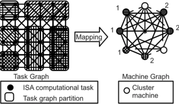
A machine graph is a representation of a cluster. Each node is a machine of the cluster. The edges are network links between the cluster’s machines. The nodes are weighted with the computational power of their associated machine. The edges are weighted with the bandwidth of their associated network link.
When the computational tasks of an ISA all have the same computational weight(an iteration of the computational task needs the same amount of instruc-tions to be completed), the computational power of a machine can be expressed as the number of computational task iterations that can be computed per second on this machine if the communications are ignored. The bandwidth is then the number of computational task data that can be sent in one second.
A task graph is a representation of an Iterative Stencil Application (ISA). Each node is an ISA computational task. Two task graph nodes are connected by an edge if their associated ISA computational tasks exchange data during the execution of the ISA. The task graph nodes are not weighted as all ISA com-putational tasks have the same comcom-putational weight. The edges are weighted with the amount of data exchanged during the ISA execution.
The load balancing problem is solved by finding an optimal mapping of the task graph onto the machine graph. The result of the mapping is the association of a task graph partition to the machine graph nodes. Each task graph node is associated to exactly one machine graph node.
1.2
Related Work
For fixed machine and task graphs, static mappers [1, 2, 3] can be used. In our case, we consider dynamic machine graphs. Static mappers are therefore not directly usable. As a new mapping has to be calculated when the machine graph changes, it must be calculated fast and during the ISA execution. Parallel algorithms can accelerate the mapping calculations. Scotch [1] and Metis [2] both feature a parallel implementation. However, these are only meant to speed up the computation of an initial static mapping.
Less attention has been paid to dynamic load balancing. However, some so-lutions exist [4, 5, 6, 7]. These methods all use iterative optimization algorithms for load balancing. Distributed implementations of these methods are easy to write. Each machine sends a message containing its current optimal workload to its neighbors. After the reception of the message of all its neighbors, a machine can update its current optimal workload. These actions are repeated until con-vergence of the optimal workloads on all machines. Work can then be migrated from overloaded to underloaded machines. The main caveat of these methods is the amount of messages that are sent before convergence is reached. Indeed, for small machine graphs (64 nodes), several thousands of iterations are needed. Several thousands of messages are therefore sent by each machine during the algorithm execution. In addition to that, only Walshaw et al.[7] solve the map-ping problem (which task on which machine). In the other methods, a machine graph node only knows how many task graph nodes will be associated to it.
2
Method description
Our load balancing method is composed of 4 phases : (1) computation of a spanning tree on the current machine graph, (2) initial homogeneous mapping of the task graph onto the machine graph, (3) load balancing of the partitions and, finally, (4) partitions refinement to minimize inter-partitions communications.
2.1
Spanning Tree Computation
Initially, each machine selects a neighborhood in the current machine graph. A spanning tree is then computed using a classical distributed algorithm [8]. This algorithm is used in the spanning tree protocol that ensures a loop-free topology for bridged local area networks. Each machine graph node has a unique ID. The root of the spanning tree is the node with the lowest ID. The distance of a node to the root is the minimal number of edges that must be followed to reach the root. The parent of a machine graph node n is the neighbor of n that is the nearest to the root. A node of the spanning tree has only one parent (except the root which has no parent). The children of n are the nodes having n as parent. Each node n of the tree is the root of a subtree T (n). |T (n)| is the size of subtree T (n) i.e. the number of nodes it contains. C(n) is the set of children nodes of n. Then |T (n)| = 1 +Pm∈C(n)|T (m)|.
The computation of the size of the subtrees starts when the spanning tree computation is finished. To compute |T (n)|, a node n must wait for the size of the subtrees associated to its children. When a subtree size |T (n)| is computed, it is forwarded to the parent of node n. The leaves do not wait data (a leaf is the root of a subtree of size 1). When the root, which has no parent, has computed the size of the entire spanning tree, initial data distribution can start.
2.2
Initial Data Distribution
The task graph is initially homogeneously distributed among the machine graph nodes. The task graph contains W nodes. If r is the root node of the machine graph spanning tree and C(r) the set of its children, the task graph will be divided into 1 + |C(r)| partitions. Each child m ∈ C(r) receives a partition of the task graph that contains (|T (m)|/|T (r)|) × W task graph nodes. The partition that is associated to r contains (1/|T (r)|) × W task graph nodes. When a machine graph node n has received its partition from its parent, it distributes it among its children using the same method. Leaf machine graph nodes keep all the task graph nodes of the partition they received from their parents. The number of task graph nodes on a machine graph node n is noted wn. The number of task graph nodes in subtree T (n) is noted Wn.
2.3
Load Balancing
Each machine graph node n is labeled with pn the power of the associated
machine. pn is expressed as the number of ISA computational task iterations
that can be computed per second on the machine associated to node n if com-munications are ignored. The computational power Pn of a subtree rooted at
node n is the sum of the computational power of all nodes of the subtree. Using the same method as for the computation of the size of all subtrees (see Section 2.1), the computational power of each subtree is computed.
From now on, each machine graph node n has the following information: its power (pn) and its number of local task graph nodes (wn), the number of
task graph nodes in each subtree rooted at the node’s children (∀i ∈ C(n) : Wi
is known) and the computational power of each subtree rooted at the node’s children (∀i ∈ C(n) : Pi is known).
The load balancing algorithm is based on the Tree Walking Algorithm (TWA) [9] initially intended for dynamic parallel scheduling. The root node of the span-ning tree calculates the average number of task graph nodes wavg = W
r/|T (r)|
per machine graph node. wavg is then broadcasted to all machine graph nodes
through the spanning tree. For each machine graph node n, a quota qn is
calcu-lated. This value indicates how many task graph nodes are to be scheduled to the machine graph node n (i.e. qn = wavg). A subtree quota is also calculated.
The subtree quota Qiis the quota associated to the subtree rooted at node i. It
is defined as follows: Qi =Pm∈T(i)qm. A machine graph node n must receive
task graph nodes from its parent if Wn < Qn. Machine graph node n must
received all awaited task graph nodes, machine graph node n sends (Wn− Qn)
task graph nodes to its parent if Wn> Qn. It also sends (Qi− Wi) task graph
nodes to each of its children i if Wi< Qi.
This algorithm does not take into account the weights of the machine graph nodes. Indeed, each machine graph node should receive an amount of task graph nodes that is proportional to the power associated to the machine. We define ln
the load of machine graph node n and Ln the load of the subtree rooted at n.
The machine graph node load ln is given by wn/pn and is expressed in seconds.
The subtree load Ln is given by Wn/Pn. The root r calculates Lr. As wavg in
the classical TWA, Lris broadcasted to all machine graph nodes. The quota of
each node is then calculated in function of Lr: qn= Lr× pn.
2.4
Partition Refinement
After the load balancing phase, the task graph nodes are associated to a machine graph node. This defines a partitioning of the task graph. The size of each partition is proportional to the power of the associated machine. However, the inter-partition communications are not minimized. A refinement phase is therefore needed.
The refinement neighborhood of a machine graph n is defined by all the ma-chine graph nodes containing task graph nodes adjacent to the task graph nodes of n. Each machine graph node exchanges task graph nodes with its refinement neighbors to decrease the edge-cut (number of task graph edges “cutting” the partition’s border). A modified version of Kernighan-Lin (KL) algorithm [10] to solve the 2-way partitioning problem is used to choose the nodes to exchange.
Given two partitions A and B, the boundary of partition A is the subset of nodes of A containing all nodes connected to a node of B. The modified version of the KL algorithm searches pairs of nodes to exchange in the boundaries of the partitions instead of the entire partitions. This strongly decreases the search time of the pair of nodes to exchange as the size of the boundary of a partition is much smaller than the partition size.
3
Dynamic Load Balancing
As stated previously, the number of nodes of the machine graph and their weights can change over time. Dynamic load balancing is therefore needed. Each time the machine graph changes, load balancing should occur. The two first phases of the method described in Section 2 can be skipped after the initial load balancing. Spanning tree computation and initial data distribution are executed only once at the beginning.
When weights of the machine graph nodes change (i.e. computational power changes), only the load balancing and the partition refinement phases are exe-cuted. When nodes are added or removed from the machine graph, the spanning tree needs partial adaptations. In the case of machine graph nodes removal, the partitions associated to these nodes must be merged with remaining partitions.
The handling of removed machine graph nodes is a fault tolerance problem. ISA fault tolerance in dynamic clusters and grids has already been investigated [11]. In this work, the ISA state (actually, the task graph and the state attached to each of its nodes) is periodically checkpointed in a distributed way. In case of fault detection, the lost states are restored on the remaining machines. In the context of our load balancing method, this means restored task graph nodes are associated to remaining partitions. After this is done, the load balancing and the partition refinement phases can be executed.
4
Results
The execution time of the presented load balancing method is measured on clusters of up to 65 machines. The method is also used to map a task graph node on a simulated heterogeneous cluster. The task graph nodes repartition on the cluster is observed after the available power of some machines is decreased.
4.1
Load Balancing Time
The load balancing time is measured from the beginning of the load balancing phase to the end of the partition refinement phase (see Section 2). The spanning tree computation and the initial data distribution are only initialization phases (see Section 3). The same task graph is mapped on clusters (machine graphs) with an increasing number of machines (machine graph nodes). The task graph contains 10000 nodes and 40000 edges. Figure 2 shows load balancing time in function of the number of machines in the cluster.
Fig. 2: Load balancing time.
The load balancing time remains roughly constant while the number of ma-chines increases. However, the real evolution of load balancing time could prob-ably be observed with more machines (up to 1000 machines and more). Unfor-tunately, we currently have no access to such clusters.
4.2
Dynamic Load Balancing
In this section, the behaviour of our load balancing method in case of avail-able computational power variations is illustrated. We simulate a cluster of 50
machines with 3Ghz processors. Initially, all the computational power is avail-able. The same task graph as in Section 4.1 is mapped on the simulated cluster. After an initial mapping, the available power of 25 machines is decreased to 2Ghz and the load balancing method is applied. The power of the same 25 machines is then decreased again to 1Ghz and our method is applied again. The initial load balancing requires all the phases described in Section 2. The two subsequent load balancings only require the two last phases (see Section 3).
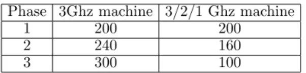
In the scenario described hereabove, there are three phases. Phase 1 features 50 × 3Ghz machines, phase 2 features 25 × 3Ghz + 25 × 2Ghz machines and phase 3 features 25 × 3Ghz + 25 × 1Ghz machines. Table 1 gives the number of task graph nodes on the machines after the initial load balancing (phase 1) and after the load rebalancings triggered by phase changes. We observed that the number of task graph nodes per machine was the same on all machines having the same power.
Phase 3Ghz machine 3/2/1 Ghz machine
1 200 200
2 240 160
3 300 100
Tab. 1: Number of task graph nodes on cluster machines for different cluster configurations.
The transition 1-2 (resp. 2-3) induces a global computational power decrease of 16% (resp. 20%). The number of moved task graph nodes in the two load rebalancings has been measured. For transition 1-2, 2457 task graph nodes are moved. As there are 10000 nodes in the task graph, this represents 25% of moved nodes. For transition 2-3, 3123 task graph nodes (31%) are moved. The majority of task graph nodes mapped on the machine graph are not moved during load rebalancing.
5
Conclusion and Future Work
In this paper, an original distributed dynamic load balancing method has been presented. It is able to map a task graph representing an ISA on a ma-chine graph representing a cluster. The described method is meant to deal with dynamic heterogeneous clusters (the number of machines and their available computational power can vary over time).
Unlike other dynamic load balancing methods [4, 5, 6, 7], load balancing is not achieved using iterative optimization methods. The amount of exchanged messages during load balancing is therefore decreased from a factor in the order of thousands. Indeed, during the load balancing phase, each node of the machine graph only sends one or two messages to its parent and children. Also, during the partition refinement phase, each node exchanges partition data with each of
its neighbors only one time.
Obtained preliminary results are encouraging. The load balancing time re-mains bounded (∼10s) for tested cluster sizes. Also, a decrease of ∼20% of the global available computation power of the cluster leads to ∼30% of moved nodes. The majority of task graph nodes are not moved during load rebalancing which is a good behaviour for a dynamic load balancing method.
It would be interesting in the future to evaluate the scalability of the proposed method. Indeed, the biggest tested cluster contained 65 machines. Clusters with thousands of machines would allow to conclude on the scalability of the method. We also plan to use the distributed load balancing method in LBG-SQUARE [11], a generic Lattice-Boltzmann based flow simulator. This would prove the usability of the method in a real application.
References
1. SCOTCH & PT-SCOTCH : Software package and libraries for graph, mesh and hypergraph partitioning, static mapping, and parallel and sequential sparse ma-trix block ordering,
http://www.labri.fr/perso/pelegrin/scotch/scotch fr.html. 2. MeTiS : Family of multilevel partitioning algorithms.
http://glaros.dtc.umn.edu/gkhome/views/metis.
3. S. Huang, E. Aubanel, V.C. Bhavsar, “PaGrid: A Mesh Partitioner for Compu-tational Grids”, Journal of Grid Computing, Vol. 4, Issue 1, pp. 71-88, march 2006.
4. G. Cybenko, “Dynamic Load Balancing for Distributed Memory Processors”, Journal of Parallel and Distributed Computing, Vol. 7, pp. 279-301, 1989. 5. R. Els˜asser, B. Monier, R. Preis, “Diffusion Schemes for Load Balancing on
Het-erogeneous Networks”, Theory of Computing Systems, Vol. 35, Issue 3, pp. 305-320, 2002.
6. C.C. Hui, S.T. Chanson, “Hydrodynamic Load Balancing”, IEEE Transactions on Parallel and Distributed Systems, Vol. 10, Issue 11, pp. 1118-1137, 1999. 7. C. Walshaw, M. Cross, M. G. Everett, “Parallel Dynamic Graph Partitioning for
Adaptive Unstructured Meshes”, Journal of Parallel and Distributed Computing, Vol. 47, pp. 102-108, 1997.
8. Radia Perlman, “An algorithm for distributed computation of a spanningtree in an extended LAN”, ACM SIGCOMM Computer Communication Review, Vol. 15, Issue 4, pp. 44-53, 1985.
9. Wei Shu, Min-You Wu, “Runtime Incremental Parallel Scheduling (RIPS) on Distributed Memory Computers”, IEEE Transactions on Parallel and Distributed Systems, Vol. 07, no. 6, pp. 637-649, June, 1996.
10. B. W. Kernighan and S. Lin, “An efficient heuristic procedure for partitioning graphs”, Bell Syst. Tech. J., Vol. 49, pp. 291-307, 1990.
11. G. Dethier, C. Briquet, P. Marchot and P.A. de Marneffe, “LBG-SQUARE - Fault-Tolerant, Locality-Aware Co-allocation in P2P Grids”, PDCAT’08, Dunedin, New-Zeland, 1-4 December 2008 (Accepted for Publication).