Urban Localization with Street Views using a Convolutional Neural Network for End-to-End Camera Pose Regression

HAL Id: hal-02156721

https://hal-mines-paristech.archives-ouvertes.fr/hal-02156721

Submitted on 14 Jun 2019

HAL is a multi-disciplinary open access

archive for the deposit and dissemination of

sci-entific research documents, whether they are

pub-lished or not. The documents may come from

teaching and research institutions in France or

abroad, or from public or private research centers.

L’archive ouverte pluridisciplinaire HAL, est

destinée au dépôt et à la diffusion de documents

scientifiques de niveau recherche, publiés ou non,

émanant des établissements d’enseignement et de

recherche français ou étrangers, des laboratoires

publics ou privés.

Urban Localization with Street Views using a

Convolutional Neural Network for End-to-End Camera

Pose Regression

Guillaume Bresson, Yu Li, Cyril Joly, Fabien Moutarde

To cite this version:

Guillaume Bresson, Yu Li, Cyril Joly, Fabien Moutarde. Urban Localization with Street Views using

a Convolutional Neural Network for End-to-End Camera Pose Regression. 2019 IEEE Intelligent

Vehicles Symposium (IV 19), Jun 2019, Paris, France. �hal-02156721�

Urban Localization with Street Views using a Convolutional Neural

Network for End-to-End Camera Pose Regression

Guillaume Bresson

, Li Yu

, Cyril Joly

and Fabien Moutarde

Abstract— This paper presents an end-to-end real-time monocular absolute localization approach that uses Google Street View panoramas as a prior source of information to train a Convolutional Neural Network (CNN). We propose an adaptation of the PoseNet architecture [8] to a sparse database of panoramas. We show that we can expand the latter by synthesizing new images and consequently improve the accuracy of the pose regressor. The main advantage of our method is that it does not require a first passage of an equipped vehicle to build a map. Moreover, the offline data generation and CNN training are automatic and does not require the input of an operator. In the online phase, the approach only uses one camera for localization and regresses poses in a global frame. The conducted experiments show that augmenting the training set as presented in this paper drastically improves the accuracy of the CNN. The results, when compared to a handcrafted-feature-based approach, are less accurate (around 7.5 to 8 m against 2.5 to 3 m) but also less dependent on the position of the camera inside the vehicle. Furthermore, our CNN-based method computes the pose approximately 40 times faster (75 ms per image instead of 3 s) than the handcrafted approach.

I. INTRODUCTION

The localization of a vehicle is a task that has raised a lot of attention lately, especially in urban environments. For autonomous driving or simply navigation, positioning a vehicle in cities has proved to be a challenging task due to urban canyons and non-line-of-sight propagation of GNSS signals. As such, many methods rely on the detection of distinctive environment features to localize a vehicle. Simul-taneous Localization and Mapping (SLAM) is the privileged method due to its ability to incrementally build a map of the surroundings while localizing the vehicle inside it. However, the application of such methods at a worldwide scale can be problematic, as detailed below.

Vehicles are supposed to be able to be localized dur-ing hundreds of kilometers of continuous drivdur-ing. Visual-based and LIDAR-Visual-based SLAM algorithms tend to drift over time due to an accumulation of errors caused by the integration of local measurements. Even the best approaches [23] exhibit an average error above 0.5% of the length of the trajectory, meaning that after 10 km, the position given by a SLAM algorithm could be 50 meters away from the real one. Countering the drift is still possible with loop closure (recognizing a previously visited place) or by integrating absolute information. The latter, under the form of GNSS measurements, are most of the time insufficient in

1_{Institut VEDECOM, 23 bis All´ee des Marronniers, 78000 Versailles,}

Francefirstname.name@vedecom.fr

2 _{Centre of Robotics, MINES ParisTech, PSL Research}

University, 60 Bd Saint Michel, 75006 Paris, France firstname.name@mines-paristech.fr

urban environments, even with differential corrections. Loop closing, even if partially correcting the drift, does not ensure that an estimation becomes drift-free [13]. It also means that the followed trajectory should regularly loop, which is rarely the case in a normal driving situation. The most viable option thus becomes to build maps beforehand using SLAM techniques, and then use the produced map as a constraint for the localization algorithm [20][11].

The main issue thus becomes the fact that these maps should be built at a worldwide scale, requiring vast fleets of equipped vehicles to do so. Even if this effort has already been initiated by mapping companies, it remains mainly focused on highways and the acquired data are not freely accessible. However, many information (especially images) are available regarding cities and urban environments as a whole. In this paper, we explore the use of Google Street View panoramas, an immense collection of images at a nearly worldwide scale, to automatically build prior environment representations that can then be used in a localization algo-rithm using a single camera. More specifically, we investigate how such a data source an be used to train a Convolutional Neural Network (CNN) to regress, in an end-to-end manner, the position and orientation of a vehicle from an image. Our contributions are the following:

• The adaptation and application of PoseNet [8] to a sparse, worldwide database of panoramas.

• The validation of the approach with real data acquired

in urban environments.

• A comparison of the results with a previously developed

approach that uses handcrafted features [21].

The rest of this paper is divided as follows: Section II exposes the related work regarding the use of existing information sources for visual localization as well as end-to-end pose regression with CNNs. Section III presents the developed method and focuses on how to build a viable training set out of Google Street View panoramas. Section IV describes the conducted experiments and the obtained re-sults in comparison to a handcrafted-feature-based approach. Finally, Section V concludes and give some insights about future works.

II. RELATED WORK

Localization is a topic that has received a lot of attention from the scientific community. Interested readers can refer to [5][4] for recent surveys. We will focus here on visual localization systems that take advantage of an existing source of information.

Visual map-aided localization systems are very few in the literature and mainly use Google Street View panoramas due

to the presence of their accurate positioning and of a coarse depth map (see Figure 1 for an example). The problem is often addressed with a place recognition objective. In [12], the authors present a ground-air place recognition system that matches aerial images with Street Views and 3D cadastral building models. Street Views are converted into a feature-based representation using Affine Scale-Invariant Feature Transform (ASIFT). A similar matching method is exploited in [19] but noisy results are removed from the trajectory with Minimum Spanning Trees (MSTs). In [22], the authors build an indexed tree based on SIFT descriptors extracted from 100,000 Street Views. A voting scheme is then used to choose the closest panorama to the query image. From a place recognition point of view, the main challenge remains to find informative enough descriptors at a city scale [3][17][18].

Regarding metric visual localization, we can cite the work of Zhang et al. [24] in which the position of the camera is estimated by triangulation between several geo-referenced Street Views. In [1], localization is performed with a two-stage approach. In the first phase, the 3D positions of tracked features in monocular sequences are estimated. Then, these estimated points are associated with Street Views in order to compute a relative transformation. Results are not directly metrically evaluated with Street Views but with recreated panoramas. Outside of Street Views, other approaches involving existing data can be found such as the use of aerial images [10] or the integration of geo-referenced objects (traffic lights and signs, for instance) to constrain the localization [16].

The rise of deep learning in perception has led to specific approaches regarding localization. For instance, the authors of [15] leverage Street View information and show that, using deep reinforcement learning, it is possible to learn how to navigate in multiple cities. The interest is not towards the accurate localization of a vehicle using Street Views but how it is possible to learn how to navigate in cities using only Steet View information. Centered on metric localization, but without using Steet Views, PoseNet [8] is an approach that uses a CNN to directly regress from a query image the corresponding 6 DoF pose. The CNN is trained from image datasets and poses generated with Structure from Motion (SfM). The results show an accuracy of a few meters (between 1.5 to 3.7 m depending on the validation test) but the convnet exhibits good robustness to changes (both illumination, weather, and presence/absence of non-static objects) and requires less computational time that a standard SfM approach. VidLoc [6] follows the same principle as PoseNet but takes into account the temporal link between images using LSTM (Long Short-Term Memory) and improves the results of PoseNet.

In this paper, we are interested in seeing how these convnets could be applied to already available data such as Street Views and thus remove the requirement of a first passage to build a database. The main drawbacks are that panoramas are far from each other (separated by 6 to 16 m) and have approximate and incomplete depth maps and

that some static elements of the scene that are needed for localization can be masked, blurred or even not up-to-date (taken in different seasons, time of day, traffic conditions, etc.).

III. DEVELOPED METHOD

As previously mentioned, we want to see how CNNs could be applied to regress a pose from an image when trained with Street View imagery. Our proposed method works in two phases. The whole pipeline is illustrated in Figure 2.

The first phase is an offline step in which Street View panoramas, along with their depth maps and absolute posi-tions, located in the test area are extracted. Panoramas are transformed into a set of rectilinear images similar in consti-tution to the images that will then be acquired in the online step (green boxes). From this initial dataset, we generate new images following the topology of the road network in order to densify the training set (gray boxes). To do so, we exploit the depth map associated to each panorama. From there, and using an adapted PoseNet architecture [8] suited to our problem, we train the convnet to regress a 2D position and orientation using the whole set of images (synthesized and real ones) and the absolute position furnished by Street View (blue box). It is worth noting that the absolute position of a Street View can be considered as accurate as it mixes several sources (SfM, GPS, odometry, IMU) in an offline manner [2].

In the online phase, the vehicle is driving inside the test area. Using only a camera, the aim is to localization the vehicle in an absolute manner. To do so, acquired images are given to the previously trained convnet which returns, as an output, the corresponding absolute 2D position and orientation of the camera.

The central aspect of this pipeline is how can sparse Street View images be used by a convnet in order to regress a proper pose. We will focus on this aspect by exposing how we augmented the original sparse Street View database with synthesized images so as to densify the training set (Subsection III-A) and how PoseNet has been adapted to fit our constraints (Subsection III-B).

A. Street View augmentation

Street View panoramas are distributed along the road network with an average distance of 6 to 16 meters in the area used in the experiments. The distance varies a lot depending on the type of environment and on the presence of intersections. In order to properly train a CNN to regress a pose from various locations, it is necessary to augment the quantity of data and their distribution along the road network where the vehicle will certainly be driving.

First, we need to be able to transform a panorama into a set of rectilinear images. To do so, we built a back projection model using ray tracing and bilinear interpolation as proposed in [14]. We create n virtual pinhole cameras, with an intrinsic calibration matrix K, located at the center O of a unit sphere S. The orientation of these virtual cameras (defined by roll (ψ), pitch (φ) and yaw (θ) angles) can be

(a) Panorama (b) Depth map (c) Depth planes in colormap

Fig. 1: Example of Street View extraction at location [48.801516, 2.131556] in Versailles, France. The depth map is computed from the given planes.

(a) Offline convnet training

(b) Online exploitation

Fig. 2: Pipeline of our approach for both automatic offline training and online exploitation. Gray boxes correspond to the Street View augmentation.

freely selected depending on the most relevant part of the panorama. A good practice is to fix ψ and φ close to the onboard camera so as to generate images with the same viewing angle and so ease the localization. We use n different θ values to generate the required amount of images in the panorama. From a 3D point P, expressed in the coordinates of the sphere S, we can compute its perspective projection p. p = K R(ψ, φ, θ)P d(R(ψ, φ, θ)P) =   fx 0 u0 0 fy v0 0 0 1   R(ψ, φ, θ)P d(R(ψ, φ, θ)P) (1) f is the focal length and (u0, v0) the principal point.

Again, these parameters are fixed according to our onboard camera. d is a function that selects the depth information

to normalize the points to a unit plan of depth equal to 1. R is the 3D rotation resulting from ψ, φ and θ. The pixel intensity is computed with bilinear interpolation.

Following this back-projection model, we are able to render images at the position where the panorama was taken. In order to distribute information along the potential trajectory of the vehicle, we need to translate the panorama (and so the sphere S) following the road network. To do so, we use the global yaw θg given in the meta-data of any

Street View and which indicates the global orientation of the vehicle when taking the panorama. We can thus compute a translation t in ENU (East-North-Up) format:

t =   l sin(θg) l cos(θg) 1   (2)

l is the Euclidian distance between the original panorama and the virtual one, expressed in a translated sphere S0. This distance can be set as needed. We can then compute the coordinates of a point P in the new translated sphere S0.

PS0 = P + R(0, 0, θ_g)t (3)

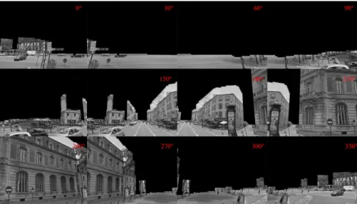
We can then create rectilinear images using Equation (1). Intensity values are interpolated from the original panorama only for points whose depth is greater than 0 when expressed in S0, otherwise we set the pixel intensity to 0. Conversely to images created from the panorama location, many pixels lack depth information when synthesized from a translated sphere. Examples of 12 images synthesized from a panorama translated 1 meter forward can be seen in Figure 3.

As can be easily spotted, some sky pixels have been synthesized. This is due to approximations in the provided depth map. The direct consequence is that it deteriorates the quality of the synthesized images. Images are rendered in grayscale to match the ones provided by the onboard camera that was used in the experiments.

We generate images following the direction of the road within a 4-meter range and with a 0.2-meter step, resulting in 40 new locations from which to synthesize images for one panorama. The 4-meter limit forward and backward has been set to limit the number of dead pixels which rises when synthesizing images far from the panorama. For each of the 41 panoramas, we create a set of 60 virtual cameras situated in the center of the sphere with θ distributed between [0; 2π[ in order to have the maximum amount of

Fig. 3: Synthesized images from a panorama translated one meter forward. Images are generated using 12 different values of yaw angle θ.

details on the environment. For the images created from the original panorama, we also generate 50 artificial brightness changes by randomly varying the value channel of a small amount (in HSV format) and 50 random shadows to simulate different sunlight conditions. Based on the whole generation scheme described here, we only keep synthesized images with a majority of non-zero pixels, leading to an augmented database that contains roughly 1500 times more images than originally.

B. PoseNet adaptation

We worked on PoseNet’s architecture [8] instead of Vid-Loc’s [6] due to the fact that our prior source of information does not directly integrate a temporal continuity between its panoramas. However, it could be worth investigating as panoramas are dated and their relative proximity gives information on the order in which they might be encountered by a moving vehicle.

PoseNet is based on a slightly modified version of GoogleNet where the softmax classifiers are replaced by affine regressors. A Fully Connected (FC) layer is added before the two regressors. The latter are responsible respec-tively for regressing the 3D position of the camera (x) and its orientation under the form of a quaternion (q). Stochastic Gradient Descent is used to train the CNN with the following loss function. L = kˆx − xk2+ β ˆ q − q kqk 2 (4) Estimations are denoted as ˆx and ˆq and the ground truth as x and q. The parameter β is used to adjust the relative weight between position and orientation errors and can be fine-tuned with grid search.

We adapted PosetNet to our problem in two ways. First, we simplified the regressor outputs in order to provide only a 2D position x2D and a global orientation θg. Positions are

projected from latitude and longitude to Universal Transverse

Mercator (UTM). We center them on the mean position of the Street View panoramas of the test area to reduce the magnitude of the values that are regressed by the CNN thus leading to the loss function defined in Eq. (5).

L = kˆx2D− x2Dk2+ β ˆ θg− θg 2 (5) We also changed the CNN architecture from GoogleNet to ResNet 50. The main reason for this change is that ResNet is better at training without overfitting with a small training dataset [7] which is our case. We modified the architecture by replacing the final classifier with the pose regressor. We also separate the regression of the 2D position and from the orientation, similarly to what is done in PoseNet. We use transfer learning to initialize the weights of convolutional layers with values from the original ResNet trained for classification on ImageNet.

IV. EXPERIMENTS AND RESULTS

The proposed method was evaluated using several acquisi-tions made in the city of Versailles, France. The vehicle was equipped with a camera and a Real Time Kinematic GNSS fused with a high-end Inertial Measurement Unit used only for ground truth purposes (accuracy of a few centimeters). Two different camera settings were tested: a camera facing forward, located inside the vehicle behind the windshield and a camera facing sideway towards building fa¸cades (see Figure 4). The camera provides grayscale images (resolution of 640×480) at 20 Hz. Two examples of images taken from the acquisitions are visible in Figure 5. It is important to note that only images were used to evaluate the method and in a pure end-to-end manner without any position tracking between two consecutive images (each frame is treated independently of the previous one).

Regarding the training phase, we used Keras and Ten-sorFlow. Every image is resized to fit the CNN input to a 224 × 224 resolution. Training is conducted with gradient descent using the Adam optimizer [9] with a learning rate of

Fig. 4: Position of the cameras in the vehicle used in the experiments.

Fig. 5: Images acquired from our vehicle in Versailles, France. Left: camera facing forward. Right: camera looking sideway.

10−5 and a batch size of 80 samples during 500 epochs. We compare the results obtained by our end-to-end pose regres-sor with our previous approach based on handcrafted features [21]. The latter uses a bag-of-words approach followed by a feature matching between the current image and the closest panoramas found. The resulting associations are then jointly optimized using bundle adjustment.

First, we validate the benefits brought by both the aug-mentation of the database and our adapted PoseNet archi-tecture using one of the acquired sequences (Sequence 1 of 234 meters) where the camera is facing sideway. Results are exposed in Table I. We can see that the augmented database considerably reduces the error in position (9.86 m against 48.13 m) but has no impact on orientation errors. It is coherent with the fact that we augment the database by creating translated panoramas. However, it also means that augmenting the number of virtual cameras does not help in estimating the orientation of the vehicle but only for its position. The changes made in the architecture of the CNN reduces again the errors regarding the position of the vehicle (7.62 m against 9.86 m) but, similarly to the augmented training set, has almost no effect on the orientation estimation. The obtained positions are plotted in Figure 6 along with the ground truth. We can observe that the trajectory jumps a lot and seems affected by a lateral offset. Jumps were expected as there is no integration of the temporal continuity of the localization in the convnet to smooth the trajectory. Regarding the lateral offset, it might be caused by an imbalanced training set as parts of the streets are more represented due the presence of depth information. Even if synthesized images with a majority of zero pixels are discarded, missing pixels could still have an impact on how the CNN interprets query images at positions where the training set was mainly constituted of images with a high amount of missing pixels.

PoseNet [8] Ours Street Views _{Street Views}Augmented _{Street Views}Augmented Training error Position (m) 8.54 0.73 0.08 Angular (◦) 1.28 1.28 0.94 Seq. 1 error Position (m) 48.13 9.86 7.62 Angular (◦) 3.34 3.79 3.55 TABLE I: Results obtained by our method and PoseNet

Fig. 6: Trajectory obtained by our method (in blue) compared to the ground truth (in red). Original panorama locations are indicated by red dots.

We evaluated our method over 5 trajectories, including 1 with the camera facing forward (and denoted Sequence F) and compared it with our previously developed approach based on handcrafted features [21]. The results are visible in Table II. Fail indicates that the handcrafted approach could not recognize the place due to many potential candidates (environment not distinctive enough) or that the training of the CNN was unable to properly converge (overfitting or underfitting observed by a validation dataset excluded from the training).

Seq. Number of Street Views Error Error of (length) images (virtual) using [21] our approach 1 (234 m) 897 29 (1160) 2.85 m 7.62 m 2 (271 m) 898 29 (1160) 2.63 m 7.93 m 3 (222 m) 895 29 (1160) Fail Fail 4 (216 m) 901 34 (1360) 2.82 m 7.55 m F (265 m) 554 29 (1160) Fail 7.87 m TABLE II: Results obtained using the proposed method and an approach based on handcrafted features [21]

Our handcrafted-feature-based approach outperforms, in terms of accuracy, our adapted PoseNet. Errors range from 2.5 to 3 meters whereas the convnet regresses position within an error of 7.5 to 8 meters. This is certainly caused by an insufficient amount of information in the generated images due to missing pixels. One solution to counter this could be to synthesize images based on several panoramas or to use Generative Adversarial Networks (GANs) to generate missing information that are mainly common elements such

as sky or vegetation. Another prospect would be to first segment the images and remove elements (put pixels to zero) for which we do not have depth information. Of course, the most obvious way to improve the performance would be to have more complete and accurate depth maps.

We can note that both approaches fail to provide a proper localization in Sequence 3. In both cases, we suspect that it is caused by dense vegetation (trees, bushes, etc.) which covers up most of the building fa¸cades where distinctive information is usually found. Localization in Sequence F, with the camera facing forward, was only possible with the convnet approach and the reached accuracy is similar to other sequences. Features were not distinctive enough to obtain a localization with the handcrafted method. Sequences 1 and F are taken in the same area thus illustrating that CNNs might offer better robustness to the position and orientation of the camera in the vehicle.

Finally, regarding computational time, with the appropriate hardware, our CNN approach takes approximately 75 ms per image whereas the approach in [21] takes 3 seconds on average to compute a position. However, it is worth noting that some parts of the processing could also be parallelized to improve the overall computational time of this approach.

V. CONCLUSION

We have presented an end-to-end approach that regresses the position and orientation of a vehicle based on a single im-age. The main contribution of our method is that the training is performed on Street View panoramas that can be extracted and processed before using the vehicle and without requiring a first passage to acquire data. We showed that it is possible to expand this sparse database of panoramas by synthesizing new images in order to help the CNN generalize the link between images and poses. We compared the results obtained by our approach in the city of Versailles, France with our previously developed method based on handcrafted features [21]. While still less accurate and globally insufficient for autonomous driving, these first results are encouraging and already roughly similar to that of a non-differential GPS, with a negligible computation time (75 ms per image, instead of 3 s for the more precise handcrafted approach).

They could be further improved. Depth maps are very coarse and do not cover all objects in the scene. It could be interesting to synthesize new images using several panora-mas. Another way to make up for missing information would be to use GANs to generate the missing pixels in the synthesized images. Adding a temporal link between panoramas could also help to reduce the sudden jumps that have been observed. One way to do that would be to use Recurrent Neural Network and to synthesize images along fake trajectories to simulate a coherent temporal continuity. Finally, one obvious modification that would improve the distinctiveness of the environment would be to use a color camera instead of a grayscale one.

REFERENCES

[1] P. Agarwal, W. Burgard, and L. Spinello. Metric Localization using Google Street View. Computing Research Repository (CoRR), 2015.

[2] D. Anguelov, C. Dulong, D. Filip, C. Frueh, S. Lafon, R. Lyon, A. Ogale, L. Vincent, and J. Weaver. Google Street View: Capturing the World at Street Level. Computer, 43(6):32–38, 2010.

[3] G. Baatz, K. K¨oser, D. Chen, R. Grzeszczuk, and M. Pollefeys. Leveraging 3D city models for rotation invariant place-of-interest recognition. International Journal of Computer Vision, 96(3):315– 334, 2012.

[4] G. Bresson, Z. Alsayed, L. Yu, and S. Glaser. Simultaneous Local-ization And Mapping A Survey of Current Trends in Autonomous Driving. IEEE Transactions on Intelligent Vehicles, 2(3), 2017. [5] C. Cadena, L. Carlone, H. Carrillo, Y. Latif, D. Scaramuzza, J. Neira,

I. Reid, and J. J. Leonard. Past, Present, and Future of Simultaneous Localization and Mapping: Toward the Robust-Perception Age. IEEE Transactions on Robotics, 32(6):1309–1332, 2016.

[6] R. Clark, S. Wang, A. Markham, N. Trigoni, and H. Wen. VidLoc: A Deep Spatio-Temporal Model for 6-DoF Video-Clip Relocalization. In IEEE Conference on Computer Vision and Pattern Recognition, 2017. [7] K. He, X. Zhang, S. Ren, and J. Sun. Deep Residual Learning for Image Recognition. In IEEE Conference on Computer VIsion and Pattern Recognition, 2016.

[8] A. Kendall, M. Grimes, and R. Cipolla. PoseNet: A convolutional network for real-time 6-DOF camera relocalization. In IEEE Interna-tional Conference on Computer Vision, pages 2938–2946, 2015. [9] D. P. Kingma and J. Ba. Adam: A Method for Stochastic Optimization.

CoRR, abs/1412.6980, 2014.

[10] R. Kummerlemmerle, B. Steder, C. Dornhege, A. Kleiner, G. Grisetti, and W. Burgard. Large scale graph-based SLAM using aerial images as prior information. Autonomous Robots, 30(1):25–39, 2011. [11] J. Levinson and S. Thrun. Robust Vehicle Localization in Urban

Envi-ronments Using Probabilistic Maps. In IEEE International Conference on Robotics and Automation, pages 4372–4378, 2010.

[12] A. Majdik, Y. Albers-Schoenberg, and D. Scaramuzza. MAV Urban Localization from Google Street View Data. In IEEE/RSJ Interna-tional Conference on Intelligent Robots and Systems, pages 3979– 3986, 2013.

[13] A. Martinelli, N. Tomatis, and R. Siegwart. Some Results on SLAM and the Closing the Loop Problem. In IEEE/RSJ International Conference on Intelligent Robots and Systems, pages 2917–2922, 2005.

[14] M. Meilland, A. I. Comport, and P. Rives. A Spherical Robot-Centered Representation for Urban Navigation. In IEEE/RSJ International Conference on Intelligent Robots and Systems, pages 5196–5201, 2010.

[15] P. Mirowski, M. K. Grimes, M. Malinowski, K. M. Hermann, K. An-derson, D. Teplyashin, K. Simonyan, K. Kavukcuoglu, A. Zisserman, and R. Hadsell. Learning to Navigate in Cities Without a Map. CoRR, abs/1804.00168, 2018.

[16] X. Qu, B. Soheilian, and N. Paparoditis. Vehicle localization using mono-camera and geo-referenced traffic signs. In IEEE Intelligent Vehicles Symposium, pages 605–610, 2015.

[17] G. Schindler, M. Brown, and R. Szeliski. City-scale location recogni-tion. In IEEE Conference on Computer Vision and Pattern Recogni-tion, pages 1–7, 2007.

[18] A. Torii, J. Sivic, and T. Pajdla. Visual localization by linear combination of image descriptors. In IEEE International Conference on Computer Vision Workshops, pages 102–109, 2011.

[19] G. Vaca-Castano, A. R. Zamir, and M. Shah. City scale geo-spatial trajectory estimation of a moving camera. In IEEE Conference on Computer Vision and Pattern Recognition, pages 1186–1193, 2012. [20] R. W. Wolcott and R. M. Eustice. Visual Localization within LIDAR

Maps for Automated Urban Driving. In IEEE/RSJ International Conference on Intelligent Robots and Systems, pages 176–183, 2014. [21] L. Yu, C. Joly, G. Bresson, and F. Moutarde. Monocular Urban Localization using Street View. In The 14th International Conference on Control, Automation, Robotics and Vision, pages 1–6, 2016. [22] A. R. Zamir and M. Shah. Accurate image localization based on

google maps street view. In 11th European Conference on Computer Vision, pages 255–268, 2010.

[23] J. Zhang and S. Singh. Visual-lidar Odometry and Mapping: Low-drift, Robust, and Fast. In IEEE International Conference on Robotics and Automation, 2015.

[24] W. Zhang and J. Kosecka. Image based localization in urban envi-ronments. In Third International Symposium on 3D Data Processing, Visualization, and Transmission, pages 33–40, 2006.