HAL Id: hal-01845977
https://hal.archives-ouvertes.fr/hal-01845977
Submitted on 20 Jul 2018
HAL is a multi-disciplinary open access
archive for the deposit and dissemination of
sci-entific research documents, whether they are
pub-lished or not. The documents may come from
teaching and research institutions in France or
abroad, or from public or private research centers.
L’archive ouverte pluridisciplinaire HAL, est
destinée au dépôt et à la diffusion de documents
scientifiques de niveau recherche, publiés ou non,
émanant des établissements d’enseignement et de
recherche français ou étrangers, des laboratoires
publics ou privés.
Impedance control using a cascaded loop force control
Sylvain Devie, Pierre-Philippe Robet, Yannick Aoustin, Maxime Gautier
To cite this version:
Sylvain Devie, Pierre-Philippe Robet, Yannick Aoustin, Maxime Gautier. Impedance control using a
cascaded loop force control. IEEE Robotics and Automation Letters, IEEE 2018. �hal-01845977�
Impedance control using a cascaded loop force
control.
Sylvain Devie, Pierre-Philippe Robet, Yannick Aoustin, and Maxime Gautier
Abstract—In this paper, a cascaded loop force control is implemented on a robot while considering the flexibility of the force sensor connecting the end effector to the tool. A classical frequency approach using a bandwidth and a phase margin is used to tune this controller. The aim is to find an equivalence between the proposed control law and a classical impedance control law. The apparent impedance of this system is calculated and can be seen as the desired impedance for a classical impedance control law. Using this equivalence the cascaded loop force controller can be tuned as an impedance controller, and can be shown to behave equivalently in simulations and experiments on a one degree of freedom (dof ) robot.
Index Terms—Force Control, Compliance and Impedance Control, Industrial Robots
I. INTRODUCTION
C
ONTROLLING the interaction with the environment is one of the most challenging fields of today’s robotics. Several applications can be considered. For example, in indus-trial applications like polishing, a robot can be used. In this case it has to apply a specific force onto the environment, while exhibiting a variable impedance. However, this paper focuses on another field of application, co-botics, where the robot has to work with a human to perform a collaborative task. The classical co-botics applications are tele-operation tasks, where the operator manipulates a master arm to perform a task with a slave arm, and co-manipulation, where the operation is executed by the robotic arm manipulated by the operator. This paper focuses on this latter application.This paper focuses on two different approaches to force control - the cascaded loop control and the impedance control. These control laws are based on the mechanical model of the robot, which is supposed to be sufficiently close to reality thanks to formal algorithms that efficiently compute robot models [1] and allow accurate identification of the dynamic parameters.
In [2], a control law was proposed to control the force and the position of a rigid robot using a stiff force sensor by decoupling force and position control using a closed loop. However, the proposed experiments showed a force overshoot
Manuscript received: September 10, 2017; Revised November 17, 2017; Accepted January 5, 2018.
This paper was recommended for publication by Editor B. Antonio and Editor R. Paolo upon evaluation of the Associate Editor and Reviewers’ comments.
The Authors are with the Universit´e de Nantes LS2N (Digital Sciences Laboratory of Nantes), 1, rue de la No¨e, ´Ecole Centrale de Nantes, France. BP 92101. 44321 Nantes, France, UMR 6004, CNRS,(Sylvain.Devie, Pierre-philippe.Robet, Yannick.Aoustin,
Maxime.Gautier)@univ-nantes.fr
Digital Object Identifier (DOI): 17-0863
at the point of impact with the environment. At the same time, impedance control was formulated by Hogan in [3] as the achievement of the desired relation between external force and robot movement. In the case of co-manipulation, it allows us to control the robot in order to control the dynamic response felt by the operator when he manipulates it. Ever since, impedance control has become the general way to control the interaction between a robot and its environment. An equivalent control law has been proposed in [4], requiring an exact model of the robot.
One of the main problems of the conventional force con-trollers is that their performances are degraded in the presence of dynamic perturbations. To solve this problem, in [5], an external force loop is proposed in order to encapsulate an inner force-based impedance loop. This external loop allows modifying the reference trajectory of the inner impedance controller online. The opposite approach was proposed by the same authors in [6]. In this paper, an inner force loop was encapsulated into an outer position-based impedance control carried out by vision. For this impedance control, the target impedance of the robot was limited to only a damping coefficient, which is also the aim of this paper. The advantage of using vision-based control is the possibility to design the two loops separately. However, this kind of controller needs a powerful processor and time to process. This is why this paper focuses on encoder-based measurement.
The classical approach to impedance control concentrates on robotic systems in which the joint elasticity is neglected. But in the case of classical industrial robots, the flexibility of the joints of the robot limit the performance of these control laws. In [7], Ott et al. proposed an impedance control law taking into account this flexibility by decoupling the dynamics of the torque from one of the links. They proposed a proof of stability and an experimental validation with a one dof robot. In [8] they proposed two controllers, using an outer impedance control loop with an inner torque loop in order to achieve the desired dynamic behaviour with respect to an external force acting on the load side. This proposed model for the robot is similar to the one defined and used by this paper. However, the flexibility considered here is the flexibility of the force sensor, which is ten times as large as that of the joints. Other approaches for impedance control considering the flexibility of the robot are presented in [9] and [10] for one dof.
The use of a one dof prismatic robot is a good solution for this kind of study, as recently shown in [11]. There, an acceleration-based impedance control law is used in a tele-operation scenario for fast environmental stiffness estimations with a time delay. In [12] a bilateral tele-operation control is
2 IEEE ROBOTICS AND AUTOMATION LETTERS. PREPRINT VERSION. ACCEPTED JANUARY, 2018
improved by considering a non-linear model for the perturba-tion observer.
In [13], a cascaded loop using proportional (P) correction for the velocity loop and proportional and integral (PI) cor-rection for the force loop is proposed. Then the equivalent impedance of the full system is calculated - it is equivalent to a apparent mass proportional to the integral correction of the system. Experiments are made for one dof of a St¨aubli RX90. In this paper, a similar control law is proposed, using a PI controller on an inner velocity loop to control the performance of the system and a P controller on an outer force loop to control the transparency of the system. The apparent impedance of the control law is a mass-damper system where the mass depends on the parameters of the PI inner velocity controller and the damper depends of the P outer force controller. This control law has been defined in a previous study [14] and applied on a known system with one dof ([15],[16],[17]).
The main contribution of this paper is to compare this control law to a classical impedance controller ([18]). The aim is to create an equivalence between the two control laws, allowing us to tune the first one [14] according to a desired impedance and tune the second one [18] according to the desired performance of the first control law. This equivalence, will allows the utilisation of the classical tool of automatism in the case of robot interacting with the environment. It will be obtained by calculating the apparent impedance of the cascaded loop control and apply it as a reference for the impedance control law. The cascaded closed loop used is an advantage because it allows us to tune the apparent mass and damping coefficient while considering the two loops independently. The stiffness term of the impedance control law will correct the errors due to the experimental conditions in an innovative manner - it is not used as a apparent stiffness like the classical impedance controller, but as a control stiffness that makes an integral term appear.
This paper is outlined as follows - Section 2 describes the experimental set-up and its modelling. Section 3 presents the closed loop controller, the calculation of its appar-ent impedance and the impedance controller targeting this impedance. Section 4 is devoted to simulations and experi-mental validations and Section 5 offers our conclusion.
II. MODELLING
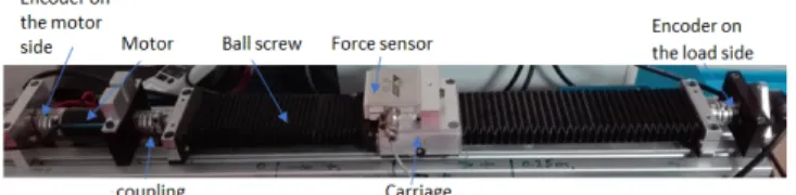
In this study, the EMPS (Electro Mechanical Positioning System) robot is considered (Fig. 1). It is a standard config-uration of a drive system for the prismatic joints of robots or machine tools. It is composed of a Maxon DC motor which drives a carriage by a Star high-precision low-friction ball screw. The carriage moves a load in translation. The motor rotor and the ball screw are connected by a flexible coupling. Two incremental encoders are present on the robot: one on the motor side and one on the load side. The first one measures the motor position and the second one measures the position of the ball screw.
In the following, let us consider that the robot is rigid in the operational frequency range, which implies that the inner
Fig. 1: EMPS robot main components
flexibility does not create oscillations. All variables are given in SI units on the load side. The motor force τ1is proportional
to the motor torque, according to the reduction ratio r of the ball screw. This torque is proportional to the electric current inside the motor according to the torque constant of the motor kt. An inner current loop is applied on the exit of the control
law. The bandwidth of this loop is sufficiently high to consider a linear relation Gi between the reference voltage of the inner
current loop vI (V) and the electric current inside the motor.
These relations allow us to write:
τ1= r.kt.Gi.vI= Gτ.vI (1)
For the following study, a tool interacting with the environ-ment is fixed to the carriage. A force sensor is used in order to measure the interaction force between the robot and the environment through this tool (Fig. 2). This sensor is a spring with a stiffness coefficient Kr12given by the manufacturer, and
this has been checked experimentally.
The mechanical system has two degrees of freedoms (dof s) : one rigid dof q1 and one flexible dof q2. The position q1
of the end effector of the robot is measured and controlled thanks to an encoder sensor. The position q2 is the relative
deformation of the force sensor spring defined in order to have τe= 0 when q2= 0, where τe is the force measured by the
sensor. It defines the position x of the end-effector thanks to (2).
x= q1+ q2 (2)
Fig. 2: Definition of the considered system. Body 1 is the controlled mass of the robot and is connected to one end of the force sensor. Body 2 is the tool, is connected to the other end of the force sensor, and interacts with the environment.
In the following, body 1 contains the moving part of the robot, including the rotor of the motor, the power transmis-sion gear and the attached end of the force sensor. Body 2 represents the other extremity of the force sensor and the tool, which is in contact with the environment.
For each body i = [1, 2], Miis the inertia, which is equivalent
to a mass in translation (kg), Fvi is the viscous damping
With respect to the reference frame fixed to the robot, the dynamic model of the horizontal mechanical device is as follows [15]:
τ1= M1q¨1+ Fv1q˙1+ Fc1sign( ˙q1) − Kr12(x − q1)
τe∗= M2x¨+ Kr12(x − q1)
(3) with τ1 the actuation force on body 1 and τe∗ the interaction
force from the environment on body 2. In the following, let us differentiate the force τe∗ applied on the system from the
environment and the force τe= Kr12(x − q1) measured by the
force sensor.
The interaction force τe∗ applied on the system and the velocity ˙x are linked by the impedance of the environment: Ze= τe∗/ ˙x. If the robot is controlled in order to apply a specific
force on the environment, Ze (N/(m/s)) is the impedance of
this environment. Three particular cases can be considered for the impedance. The softest case is the free case: τe∗= 0 so
Ze= 0, which means that there is no obstacle and the robot is
free to move. The hardest case is the constraint case: ˙x= 0 so Ze−→ ∞, which means that the environment is an infinitely
rigid obstacle, the direct consequence is that x is constant.
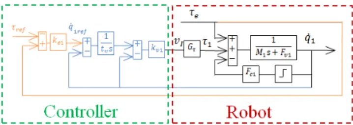
Fig. 3: Cascaded closed loop of speed (blue) and force (orange) in the case of co-manipulation.
III. CONTROL DESIGN
A. Cascaded loop control
The previous study [14], a simple control law was studied for the force control using an IP correction for the velocity loop and a P correction for the force loop. Then, this control law was adapted in order to perform the co-manipulation task. In the co-manipulation case, the environmental impedance depends on the impedance of everything interacting with the robot, including the environment and the operator’s hands, it is supposed to be unknown. In this case, the control system is illustrated in Fig. 3. The velocity loop is used to control the performance of the system and the force loop is mostly used to control its transparency. Here, by increasing the gain ke1,
we increase the transparency. However, a very high gain can lead to instability. We consider τre f the desired effort applied
by the robot on the operator’s hand, it can be seen as an offset of effort that the operator has to apply. In order get an easy co-manipulation with τe= 0 when the robot is not moving
( ˙q1= ˙q2= 0), we choose τre f= 0.
Thanks to this reference, the system allows a linear re-lationship between the external force τe and the velocity
reference ˙qre f. If the external perturbation has a low frequency,
the relation τe= kcq˙1 can be used in order to calculate the
correction gain of the closed loops.
In the following, we consider M2x¨ τe∗. In this case we
have τe∗= τe. In this case, (3) becomes (4).
τ1= M1q¨1+ Fv1q˙1+ Fc1sign( ˙q1) − τe∗ (4)
In order to calculate the correction and the performance of the system, we consider that the frequency range of τe
(< 20 rad/s) is small compared to the bandwidth of the velocity loop (100 rad/s), giving us a linear relation between the velocity and the external force: τe= kcq˙1with kc= 1/ke1.
Imposing the phase margin φv at a frequency ωv leads to
Tvo( jωv) = q˙ q˙1
1re f− ˙q1 = 1e
j(−π+φv) and gives the values of k
v1
and tv. The closed velocity loop is defined with a transfer
func-tion of second order, the cut-off frequency ω0v=
p
Kv/M1and
a damping coefficient zv= (tv+KCv)ω20v, with Kv= kv1Gτ/tv
and C = Fv1− kc.
According to Fig. 3 and considering a reference for τre f= 0
for co-manipulation applications, the open loop transfer func-tion of the velocity loop is given by the equafunc-tion:
Tvo(s) = ˙ q1(s) vq˙(s) − ˙q1(s) =kv1Gτ tvs 1 M1s +C + kv1Gτ (5) with C = Fv1−kc. Imposing the phase margin φvat a frequency
ωv leads to Tvo( jωv) = 1ej(−π+φv) and gives the values of kv1
and tv. This criterion ensures the stability of the system and
allows to calculate some characteristics of the control, like the overshoot of the response time. However, the passivity analysis, which is currently used in case of robot/environment interaction only assure the stability, it is not necessary here. B. Equivalent impedance
The apparent impedance of the robot is the impedance felt by the operator when he manipulates the robot. By separately considering the two blocks of Fig. 3, it is possible to write the following equation: Z1(s) = τ1(s) + τe(s) ˙ q1(s) τ1(s) = A(s)τe(s) − B(s) ˙q1(s) (6) with:
• Z1= (M1s + Fv1) the impedance of the robot, • A(s) =ke1kv1Gτ tvs = Kv kcs • B(s) = kv1Gτ 1 + tvs tvs = Kv 1 + tvs s .
Let us now define the equivalent impedance of the robot from (6): Zr= τe ˙ q1 (s) =Z1+ B(s) A(s) + 1 (7) This equation can be written in the following form:
Zr= kc
M1s2+ (Fv1+ Kvtv)s + Kv
kcs + Kv
(8) At low frequencies ω Kv/kc, which is in the frequency
range of our applications, the denominator of (8) is equivalent to a gain Kv. Similarly, for ω
p Kv/M1 we simplify the numerator to get: Zr= kc (Fv1+ Kvtv)s + Kv Kv (9)
4 IEEE ROBOTICS AND AUTOMATION LETTERS. PREPRINT VERSION. ACCEPTED JANUARY, 2018
According to the previous section: tv= 2zv ω0v −Fv1− kc Kv (10) Zr= 2zvkc ω0v (1 + kc 2zvω0vM1 )s + kc (11)
So we can define the apparent impedance as Zr= Mas + Fva,
with: • Ma= 2zvkc ω0v (1 + kc 2zvω0vM1
) the apparent mass,
• Fva= kcthe apparent damping.
This simplified impedance is equivalent to the one of eq. (8) in the considered frequency range, as shown in Fig. 4. The numerical value of the mechanical parameters are given in the following section. We use this simplified assumption in the remainder of this paper.
Fig. 4: Bode diagram of the apparent impedance of (8) and its simplified version (11), the numerical values of the parameters are defined in the next section.
From this control law, no stiffness coefficient K0 can be
identified. However, it would be possible to identify such a stiffness with another kind of cascaded loop. For example, adding a position loop in parallel to the force loop allows us to define an apparent stiffness K0. However, the control law
presented in this paper behaves like a mass damper system and does not use any apparent stiffness other than the stiffness of the force sensor. Hence in order to ensure the equivalence between the two control laws, the stiffness coefficient K0will
be considered null in the first set of experiments below. However, the apparent impedance of the robot at the point of interaction with the environment is Za= τe∗/ ˙x. It should not be
confused with Ze which is the impedance of the environment
at the point of interaction with the robot. According to the second equation of (3): ˙ q1(s) = sq1(s) = s Kr12 (Z2x(s) − τ˙ e∗(s)) (12)
with Z2= M2s + Kr12/s, (11) and (12) give:
Zr=
τe∗ Z2x− τe∗
Kr12
s (13) The expression of Zabecomes:
Za=
ZrZ2
Kr12
s + Zr
(14)
When M2x¨can be neglected with respect to τe∗, which is the
case in the considered applications, this equation becomes: Za= Zr 1 + Zr Kr12 s (15) This means that the apparent impedance strongly depends on the stiffness of the force sensor measuring the interaction between the robot and the environment. If this stiffness has high values, Zais equivalent to Zr. If this stiffness has very low
values, τe∗ is not transmitted to the robot and it is equivalent to a low pass filter.
C. Impedance control
Let us now consider an impedance control. From (4), we get:
τ1+ τe∗= M1q¨1+ Fv1q˙1+ Fc1sign( ˙q1) (16)
The considered model for the impedance control is given by Fig. 6. The goal here is to control the robot in order to give it a specific apparent inertia Za= τe∗/ ˙x. However, at
low frequencies, ˙x≈ ˙q1. This is the case when the resonance
frequency of the robot pKr12/M1 is low compared to ωv.
Usually, this impedance is chosen to have the following desired behaviour:
τe∗= Maq¨1+ Fvaq˙1+ K0(q1− q10) (17)
q10 is the position reference for the impedance controller. The
gain K0 is usually chosen according to the desired apparent
stiffness Ka, with
Ka−1= K0−1+ Kr12−1 (18) According to this equation, the apparent stiffness cannot be higher than Kr12. However, in this specific case, the apparent
stiffness was not identified in the precedent section. It will be calculated in another method in the next section. Let us define the acceleration ¨q1: ¨ q1= 1 Ma (τe∗− Fvaq˙1− K0(q1− q10)) (19)
By substituting (19) into (16), the controlled force is: τ1= (τe− τre f) M1− Ma Ma + (Fv1− Fva M1 Ma ) ˙q1 −K0 M1 Ma (q1− q10) + Fc1sign( ˙q1) (20) The main focus of this study is to compare the behaviour of the system controlled by this force to the one controlled by the cascaded loop represented in Fig. 3.
Let us now verify whether the apparent impedance of this control law corresponds with the one presented in the previous section. By injecting (20) into (4) with τre f = 0, we get the
equation represented in Fig. 5. It can be simplified into: τe= Maq¨1+ Fvaq˙1+ K0
M1
Ma
(q1− q10) (21)
According to this equation, we get Zr= τe/ ˙q1= Za, with Za
defined in (15) at low frequency. If this apparent impedance is considered, both control laws are equivalent.
Fig. 5: Impedance closed loop in the case of co-manipulation.
Fig. 6: Definition of the considered system for the impedance control.
Here, Ma and Fva are chosen from the expression of Zr in
the previous section in order to have a correlation between the two control laws. The gain K0is chosen equal to 0 N/m.
IV. EXPERIMENTAL VALIDATION AND DISCUSSION
The EMPS robot is used. This robot was fully identi-fied in previous studies [15], the numerical values of the parameters used in the previous section are: M1= 105 kg,
Fv1 = 212 N/(m/s), Fc1 = 18.5 N, Gτ = 35 N/V and
Kr12= 2 104 N/m. The considered mass M1is the equivalent
mass of the robot, including the parts moving in rotation, like the rotor, and the parts moving in translation, like the carriage. The position of the payload is calculated thanks to the encoder sensor and a backward derivative is used to calculate the velocity.
First of all, a simulation will be presented in order to compare the effects of the two control laws on a system that is perfectly known. Then these control laws will be tested on hardware.
A. Simulations
Let us consider the following scenario: the robot is free to move and an operator applies a specific force τe on the
end-effector. This force is measured by the force sensor and used to control the robot. Then, the evolution of the velocity of the robot is observed in order to compare the two control laws. The system is simulated thanks to Simulink in order to compare the two control laws in a controlled environment, using the parameters of Table I.
TABLE I: Parameters of the first set of experiments
Dynamic parameters closed loop gains apparent impedance zv=
√
2 kv1= 7.5 102 Ma= 9 kg
wv= 100 rad/s tv= 2.8 10−2s Fva= 323 N/(m/s)
kc= 323 N/(m/s) ke1= 3.1 10−3 K0= 0 N/(m/s)
The aim of these simulations is to show the equivalence between both control laws, supposing the robot is perfectly identified. Here, the stiffness K0 does not appear in the
apparent impedance of the cascaded loop, so it is chosen to be equal to zero in the case of impedance control. The Coulomb friction in the robot is equivalent to a constant perturbation, which is compensated by the integral correction in the case of the cascaded loop. However, in the case of impedance control, a friction compensation is applied instead. For the experiments on the real system, this is not possible because of the identification error of the friction model (up to 5%). Thus a specific integration will be discussed in the experimental part. Simulations were performed with these parameters for the two control laws. For the first one, a step signal was applied for the force τeand the evolution of the velocity ˙q1was observed.
The evolution of this velocity is presented in Fig. 7a for the two control laws. The goal is to design a control with an apparent impedance equals to the desired damping factor Fva=
kc, similar to [6].
(a) Velocity for the two control laws for a step input.
(b) Velocity amplitude, as a func-tion of the force input frequency for the two control laws.
Fig. 7: Simulation: Velocity, for a force input. Fig. 7 shows that, for the same input, the velocity in steady state is the same for the two control laws. The response time to reach 5% of the final value is 76 ms for the closed loop control law and 85 ms for the impedance control law. However, the velocity obtained with the closed loop control law has a second order transfer function behaviour during the transitional time. On the other hand, the velocity obtained with the impedance control law has a first order transfer function behaviour during
6 IEEE ROBOTICS AND AUTOMATION LETTERS. PREPRINT VERSION. ACCEPTED JANUARY, 2018
the transitional regime. This difference is not very visible in Fig. 7a because the damping coefficient zv was chosen to be
larger than 1.
Other simulations were executed with these parameters in order to check the bandwidth of these control laws. The parameters of Table I were applied to the two control laws and a sinusoidal function was used for the force input. In this configuration, Fig. 7b shows the evolution of the velocity amplitude as the frequency of the input increases. This figure shows that, if the bandwidth of the impedance control law (4 Hz) is similar to the one of the cascaded loop control law (4 Hz), their velocities are very close. These results prove the equivalence of the two control laws for this specific configuration. According to several simulations, the response of the two controls laws are the same during the transitional regime, with a maximum difference of 10 ms for the response time. But if the damping coefficient zv is reduced to below
1, the response of the control law using the cascaded loop should decrease and have an overshoot, which is the classical behaviour of a second order closed loop, while the response of the impedance closed loop should keep its first order behaviour. However the behaviour at steady state is the same and the maximal difference for the time response is up to 15 ms for a damping coefficient of √2/2. So, even if the behaviour is slightly different during the transitional regime the equivalence between the two control laws is valid for any damping coefficient.
B. Experiments
Experiments were performed with the parameters presented in Table I on the EMPS robot. The main difficulties appearing for the comparison of the two control laws in co-manipulation is that the action from the operator is not perfectly repeatable. However, the force τe applied by the operator is far smaller
than the force τm applied by the motor. Because of this
assumption, the effort from the environment can be neglected in the dynamics of the body 1. The input of the control law is divided into the force from the operator and the force from the environment. We choose to simulate the action from the operator, and to consider the effort from the environment to be equal to the one measured by the force sensor. For the experiments, the robot is placed in front of a stiff obstacle.
In the first case, the stiffness K0is still considered equal to
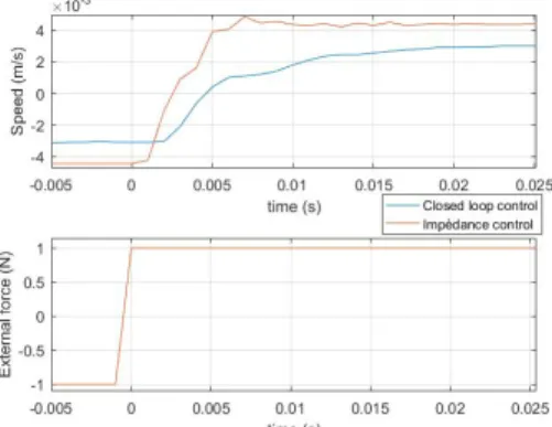
0 N/m in order to make a comparison of the two control laws. The input force has values equal to 1 N for t > 0 and −1 N for t < 0. This specific input allows us to use a square signal for the reference force, and to easily repeat the experiment. The evolutions of the velocity ˙q1and the external force τeare
showed in Fig. 8 for the two control laws.
According to this figure, the response time of the impedance control law is half of the one from the cascaded loop control law, and the steady state behaviour is not the same for the two control laws. This difference is mostly due to the approximation of the friction parameters. Actually, in the case of the EMPS robot, the approximation of the Coulomb and viscous damping has a maximal accuracy of 2 N, which is the order of magnitude of the force applied on the robot. In order
Fig. 8: Evolution of velocity for the two control laws for a step input, during the transitional time without environmental reaction, with K0= 0.
to have the same behaviour for the two control laws, an integral correction has to be applied in the impedance control law in order to track the reference position q10. We decided to build
this integral correction using the unidentified coefficient K0.
Here, we do not consider a desired stiffness for the dynamic behaviour of the system, but a control stiffness K0 around
a position q10 defined from the measurement of the external
force by:
q10=
Z t 0
ke1τe(u) du (22)
Three values were considered for the stiffness K0 in order to
be stable and have a behaviour similar to the cascaded loop in transitional regime. These values are of the order of magnitude of the stiffness of the force sensor and can be expressed as a function of it: Kr12, Kr12/2 and Kr12/3. The evolution of the
velocity, for no environmental reaction is shown in Fig. 9
Fig. 9: Velocity for the two control laws for a step input, during the transitional time without environmental reaction, with differents values for K0.
As shown in this figure, the behaviour of the robot con-trolled with the closed loop control law is coherent with the simulation results: the high damping coefficient allows no overshoot, the integral correction leads us to null steady state error and the response time to 5% of the final value is equal to 86 ms thanks to the chosen dynamics. For the impedance control, it appears that the choice of the gain K0
has a significant influence on the dynamics of the system. Taking this parameter to be equal to Kr12 leads us to feel an
apparent stiffness equal to Kr12/2, but the velocity response
presents an overshoot because of the rigidity of the system. On the other hand, a coefficient K0 that is too low decreases
the performance of the controller. A good match between the two control laws is obtained for K0= Kr12/2. In this case, the
apparent stiffness is equal to Kr12/3. Similar to the cascaded
loop control law, this one presents no overshoot. It has a response time equal to 88 ms.
Fig. 10: Velocity for the two control laws for a step input for the full experiment, including the contact phase with a stiff obstacle.
The evolution of the velocity ˙q1 and the external forces
are shown in Fig. 10 when the robot is in contact with the stiff obstacle. In this case, all the control laws present the same behaviour. In steady state, before touching the obstacle, the velocity is constant and equal to ke1τe. Then, when the
end-effector touches the stiff obstacle, the velocity decreases to zero with a first order transfer function behaviour. During this operation, the curves of the velocities from all the control laws are superimposed and have a response time that is far longer than the one of the free phase. During this phase, the dynamics of the system depend on the obstacle, which is stiffer than the force sensor. A rigid wall is present on the other side of the stiff obstacle. The response shown in Fig. 10 during these phases depends on the equivalent stiffness of the Robot + Obstacle system, which is almost the same for the four control laws.
These experiments show that the control law proposed using a cascaded closed loop is equivalent to an impedance control law using apparent mass and damping, which can be calculated according to the parameters of the control law, and an apparent stiffness which can be built in order to add an integral correction to the basic impedance control law.
V. CONCLUSION
In this paper, a force control law using a cascaded loop was presented in order to perform a co-manipulation task. The apparent inertia of a specific robot using this control law was calculated and used in order to make an impedance control law. It appears that the apparent mass and the apparent damping
of this impedance can be calculated according to the dynamic parameters of the robot.
Simulations proved the equivalence between these two control laws under certain assumptions and the experiments showed the limit of this equivalence. However, it is possible to push these limits by building an integral correction in the impedance control law.
ACKNOWLEDGEMENTS
The project is co-funded by the European Union. Europe is now investing in Pays de la Loire with the European Regional Development Fund.
REFERENCES
[1] W. Khalil, J. Kleinfinger, and M. Gautier, “Reducing the computational burden of the dynamic models of robots,” in IEEE Int. Conf. on Robotics and Automation, pp. 525–531, 1986.
[2] O. Khatib and J. Burdick, “Motion and force control of robot manip-ulators,” IEEE Int. Conf. on Robotics and Automation, vol. 3, no. 5, pp. 1381–1386, 1986.
[3] N. Hogan, “Impedance Control: An Approach to Manipulation,” J. of Dynamic Systems, Measurement, and Control, vol. 107, no. March, pp. 304–313, 1985.
[4] A. A. Goldenberg, “Implementation of force and impedance control in robot manipulators,” IEEE Int. Conf. on Robotics and Automation, vol. 3, pp. 1626–1632, 1988.
[5] G. Morel and P. Bidaud, “A reactive external force loop approach to control manipulators in the presence of environmental disturbances,” IEEE Int. Conf. on Robotics and Automation, vol. 2, no. April, pp. 1229– 1234, 1996.
[6] G. Morel, E. Malis, and S. Boudet, “Impedance based combination of visual and force control,” IEEE Int. Conf. on Robotics and Automation (Cat. No.98CH36146), vol. 2, no. May, pp. 1743–1748, 1998. [7] C. Ott, A. Albu-Schaffer, A. Kugi, and G. Hirzinger, “Decoupling based
Cartesian impedance control of flexible joint robots,” IEEE Int. Conf. on Robotics and Automation, vol. 3, no. July, pp. 671–683, 2003. [8] C. Ott, A. Albu-Schaffer, A. Kugi, and G. Hirzinger, “On the
Passivity-Based Impedance Control of Flexible Joint Robots,” IEEE Trans. on Robotics, vol. 24, no. 2, pp. 416–429, 2008.
[9] R. Ozawa and H. Kobayashi, “A new impedance control concept for elastic joint robots,” IEEE Int. Conf. on Robotics and Automation, vol. 3, pp. 26–31, 2003.
[10] G. Ferretti, G. A. Magnani, and P. Rocco, “Impedance control for elastic joints industrial manipulators,” IEEE Trans. on Robotics and Automation, vol. 20, no. 3, pp. 488–498, 2004.
[11] D. Yashiro, “Fast Stiffness Estimation using Acceleration-based Impedance Control and its Application to Bilateral Control,” in IFAC World Congress, pp. 12565–12570, 2017.
[12] K. Seki, S. Fujihara, and M. Iwasaki, “Improvement of Force Trans-mission Performance Considering Nonlinear,” in IFAC World Congress, pp. 12577–12582, 2017.
[13] X. Lamy, F. Colledani, F. Geffard, Y. Measson, and G. Morel, “Achieving efficient and stable comanipulation through adaptation to changes in human arm impedance,” in IEEE Int. Conf. on Robotics and Automation, pp. 265–271, 2009.
[14] S. Devie, P. P. Robet, Y. Aoustin, M. Gautier, and A. Jubien, “Accurate force control and co-manipulation control using hybrid external com-mand,” IFACWorld Congress, pp. 2271–2276, 2017.
[15] M. Gautier, A. Jubien, A. Janot, and P. P. Robet, “Dynamic Identification of flexible joint manipulators with an efficient closed loop output error method based on motor torque output data,” in IEEE Int. Conf. on Robotics and Automation, pp. 2949–2955, 2013.
[16] P. Hamon, M. Gautier, P. Garrec, and A. Janot, “Dynamic Modeling and Identification of Joint Drive with Load-,” in Int. Conf. on Advanced Intelligent Mechatronics, pp. 902–907, 2010.
[17] P. P. Robet and M. Gautier, “Cascaded loops control of DC motor driven joint including an acceleration loop,” in IFAC World Congress, (Cape Town, South Africa), pp. 513–518, 2014.
[18] N. Hogan, “Stable execution of contact tasks using impedance control,” IEEE Int. Conf. on Robotics and Automation, vol. 4, pp. 1047–1054, 1987.