HAL Id: hal-00670641
https://hal.archives-ouvertes.fr/hal-00670641
Submitted on 15 Feb 2012
HAL is a multi-disciplinary open access
archive for the deposit and dissemination of
sci-entific research documents, whether they are
pub-lished or not. The documents may come from
teaching and research institutions in France or
abroad, or from public or private research centers.
L’archive ouverte pluridisciplinaire HAL, est
destinée au dépôt et à la diffusion de documents
scientifiques de niveau recherche, publiés ou non,
émanant des établissements d’enseignement et de
recherche français ou étrangers, des laboratoires
publics ou privés.
A Similarity Skyline Approach for Handling Graph
Queries - A Preliminary Report
Katia Abbaci, Allel Hadjali, Ludovic Liétard, Daniel Rocacher
To cite this version:
Katia Abbaci, Allel Hadjali, Ludovic Liétard, Daniel Rocacher. A Similarity Skyline Approach for
Handling Graph Queries - A Preliminary Report. International Workshop on Graph Data Management
Techniques and Applications (GDM’11), in Conjunction with The IEEE International Conference on
Data Engineering (ICDE)„ Apr 2011, Germany. pp.112-117. �hal-00670641�
A Similarity Skyline Approach for Handling Graph
Queries - A Preliminary Report
Katia Abbaci
#1, Allel Hadjali
#2, Ludovic Li´etard
∗3, Daniel Rocacher
#4,
#IRISA/ENSSAT
Rue de K´erampont BP 80518 Lannion, France 1[email protected] 2[email protected] 4[email protected]
∗IRISA/IUT
Rue Edouard Branly BP 30219 Lannion, France 3[email protected]
Abstract—One of the fundamental problems in graph databases is similarity search for graphs of interest. Existing approaches dealing with this problem rely on a single similarity measure between graph structures. In this paper, we suggest an alternative approach allowing for searching similar graphs to a graph query where similarity between graphs is rather modeled by a vector of scalars than a unique scalar. To this end, we introduce the notion of similarity skyline of a graph query defined by the subset of graphs of the target database that are the most
similar to the query in a Pareto sense. The idea is to achieve a
d-dimensional comparison between graphs in terms of 𝑑 local distance (or similarity) measures and to retrieve those graphs that are maximally similar in the sense of the Pareto dominance relation. A diversity-based method for refining the retrieval result is proposed as well.
I. INTRODUCTION
Graphs have become increasingly important in modeling complex structured data in many recent real applications. These applications include Bioinformatics [1], [2], Pattern Recognition [3], XML documents [4], Chemical compounds [5], Social networks [6], etc. All these applications indicate the importance and the broad usage of graph databases. One can broadly classify queries against graph databases into two categories [7]: (1) Graph containment search and (2)
Graph similarity search. The former consists of the following
two sub-problems: (i) subgraph containment search: given a graph database 𝐷 = {𝑔1, 𝑔2, . . . , 𝑔𝑛} and a graph query q, retrieve all graphs 𝑔𝑖 ∈ 𝐷 such that q is a subgraph of 𝑔𝑖 (i.e., 𝑞 ⊆ 𝑔𝑖); (ii) supergraph containment search: given a graph database 𝐷 = {𝑔1, 𝑔2, . . . , 𝑔𝑛} and a graph query q, retrieve all graph 𝑔𝑖 ∈ 𝐷 such that q is a supergraph of 𝑔𝑖 (i.e., 𝑞 ⊇ 𝑔𝑖). Both sub-problems consider the procedure of checking subgraph isomorphism, known to be NP-Complete. Many query processing approaches using indexing techniques have been developed to reduce the search space and then efficiently solve these two sub-problems [8], [9], [10], [11].
As for the second category (i.e., graph similarity search), which consists in retrieving all the graphs of the database that are structurally similar to a given graph query, has emerged
as new trend due to the following reasons [12], [13]. Firstly, many real graph datasets are noisy and incomplete in nature, so approximate, rather than exact, graph matching is required. Secondly, many graph applications prefer approximate match-ing results rather than exact ones as they can provide more information such as what might be missing or spurious in a query or in a graph database. A number of approaches therefore have been proposed to support similarity queries on graph databases, see [14], [15] and [12] in the case of subgraph queries and [16] in the case of supergraph queries. The common point of all those approaches is the fact that they impose a single measure to evaluate graph similarity. However, a graph is a complex structure by nature and involves various basic features. It is then difficult to give a meaningful definition of graph similarity using only a single index.
In this paper, we advocate that for graph similarity to be efficiently assessed, several indices are required. Each index is dedicated to measure a local distance (or similarity) between two graphs pertaining to one aspect in the graph structure. Therefore, graph similarity is now characterized by a vector of local distance measures (where each measure expresses a feature similarity) instead of a single measure. By this way, one can preserve information about similarity on several features when comparing two graphs.
We propose an approach based on the notion of similarity skyline to support graph similarity search. Roughly speaking, the similarity skyline of a graph query is defined by the subset of graphs of the target database that are the most similar to the query in a Pareto sense. The idea is to achieve a d-dimensional comparison between graphs in terms of d local distance (or similarity) measures and to retrieve those graphs that are maximally similar in the sense of a defined
similarity-dominance relation. In summary, we made the following
contributions in this paper:
∙ We introduce the notion of graph compound similarity and then define the similarity-dominance relationship between graphs.
of the graph similarity skyline, i.e., graphs of the target database that are maximally similar to a graph query in a Pareto sense.
∙ To reduce the resulting skyline (which is often quite large), we propose a method to extract a subset which is as diverse as possible, but with an acceptable size. The rest of the paper is organized as follows. Section 2 provides some preliminary notions. Related work is discussed in Section 3. Section 4 describes some well-known measures for graph similarity and their semantic properties. In Section 5, we introduce the notion of similarity skyline to support graph similarity queries. Section 6 proposes a detailed example. Section 7 presents a method for refining the retrieval result. Section 8 concludes the paper.
II. PRELIMINARIES A. Reminder About Skyline Queries
Skyline queries [17] are a popular and powerful paradigm for extracting interesting objects from a multi-dimensional dataset. They rely on Pareto dominance principle which can be defined as follows:
Definition 1. Let r be a set of d-dimensional data points
and 𝑝 = (𝑝1, 𝑝2, . . . , 𝑝𝑑) and 𝑞 = (𝑞1, 𝑞2, . . . , 𝑞𝑑) two points of r. p is said to dominate (in the Pareto sense) q iff on every dimension 𝑝𝑖 ≤ 𝑞𝑖 (for 1 ≤ 𝑖 ≤ 𝑑) and on at least one dimension 𝑝𝑗 < 𝑞𝑗.
For simplicity and without loss of generality, we assume that the smaller the value 𝑝𝑖, the better. We say then that p
dominates (is preferred to) q and we denote this by 𝑝 ≻ 𝑞. Definition 2. The skyline of r is the set of points which are
not dominated by any other point.
Skyline queries compute the set of Pareto-optimal tuples in a relation, i.e., those tuples that are not dominated by any other tuple in the same relation.
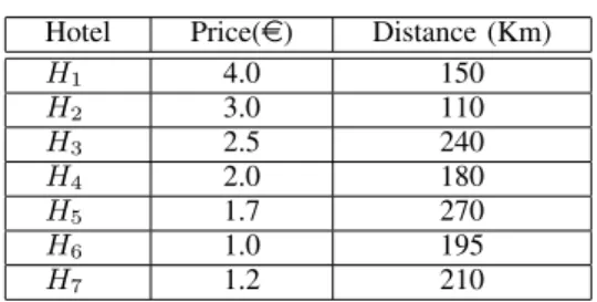
Example 1. Consider a database containing information
about hotels as shown in Table I (where dimension d = 2).
TABLE I SAMPLEHOTELS
Hotel Price(e) Distance (Km)
𝐻1 4.0 150 𝐻2 3.0 110 𝐻3 2.5 240 𝐻4 2.0 180 𝐻5 1.7 270 𝐻6 1.0 195 𝐻7 1.2 210
Consider a person who looks for a hotel that is as close as possible to the beach and having a low price. One can check that the resulting skyline S contains 𝐻2, 𝐻4 and 𝐻6. For instance, 𝐻1is dominated by 𝐻2, and𝐻7by 𝐻6.
B. Some Basic Definitions
Definition 3 (Graph). A graph g is defined as a 4-tuple (V, E, L, l) where V is the set of vertices, E is the set of edges, L
is the set of labels and l is a labeling function that maps each vertex or edge to a label in L.
For ease of presentation, graphs refer here to undirected labeled graphs. Note that different nodes could have the same label and the size of g is defined as∣𝑔∣ = ∣𝐸(𝑔)∣ (i.e., the size of a graph is the number of its edges).
Definition 4 (Graph isomorphism). Given two graphs g = (V, E, L, l) and g’ = (V’, E’, L’, l’), g is isomorphic to g’
(denoted by 𝑔 ≈ 𝑔′) if there exists a bijection 𝑓 : 𝑉 → 𝑉′, such that
1) ∀𝑣 ∈ 𝑉, 𝑓(𝑣) ∈ 𝑉′ and l(v) = l’(f(v)) and;
2) ∀(𝑢, 𝑣) ∈ 𝐸, (𝑓(𝑢), 𝑓(𝑣)) ∈ 𝐸′, and l(u, v) = l’(f(u), f(v)).
Definition 5 (Subgraph isomorphism). Given two graphs g = (V, E, L, l) and g’ = (V’, E’, L’, l’), g is subgraph isomorphic to g’ if there exists an injection𝑓 : 𝑉 → 𝑉′ such that
1) ∀𝑣 ∈ 𝑉, 𝑓(𝑣) ∈ 𝑉′ and l(v) = l’(f(v)) and;
2) ∀(𝑢, 𝑣) ∈ 𝐸, (𝑓(𝑢), 𝑓(𝑣)) ∈ 𝐸′ and l(u, v) = l’(f(u), f(v)).
Definition 6 (Subgraph v.s. supergraph). Given two graphs g = (V, E, L, l) and g’ = (V’, E’, L’, l’), g is called a subgraph of g’ (or g’ is a supergraph of g), denoted as𝑔 ⊆ 𝑔′ (or𝑔′⊇ 𝑔), if there exists a subgraph isomorphism from g to g’.
Definition 7 (Maximum common subgraph, mcs). Given two
graphs𝑔1and𝑔2, the maximum common subgraph of𝑔1and𝑔2 is the largest (i.e., the maximum number of selected vertices) connected subgraph of 𝑔1 that is subgraph isomorphic to 𝑔2, denoted as𝑔′= 𝑚𝑐𝑠(𝑔1, 𝑔2).
III. RELATEDWORK
Our proposal can be related to the works in the areas of skyline queries and similarity queries on graph databases.
Skyline queries. They have received a lot of attention over
the recent years. Several research efforts have been made to develop efficient algorithms and to introduce different variants for skyline queries [18], [19], [20], [21]. Up to our knowledge, no work related to skyline queries exists in a graph data context, except the recent work by Zou et al. [22] where dynamic skyline queries in a large graph have been studied. In our case, a different kind of skyline (i.e., similarity skyline) over a set of graphs (rather than a single large graph) is investigated.
Similarity queries. Similarity search of graphs is a vital
operation in many recent applications. As indicated in Section I, this kind of graph search is conducted thanks to similarity queries that aim at finding graphs in the target database that are similar, but not necessarily isomorphic, to a given graph query. A number of approaches have been developed to support similarity queries. Grafil [14] performs substructure similarity search in a large scale graph database. It returns all the graphs of the database that approximately contain the graph query. C-Tree [15] is another tool for subgraph similarity search which focuses on the edit distance between the query and its candidate matches. Tale [12], unlike most previous graph matching tools which treat every node in a
graph equally, proposes an innovative matching technique that distinguishes nodes by their importance in the graph structure. This technique first matches the important nodes of a graph query, and then progressively extends these matches. Recently, Shang et al. [16] have proposed a technique to deal with supergraph queries where the notion of maximum common subgraph plays a key role. The problem of interest is converted into a 𝜎-missing subgraph detection problem, where 𝜎 is the error tolerance threshold. All the graphs of the queried database such that the mcs-based distance measure to the graph query considered is less than𝜎, are returned as answers. Both
C-Tree and Tale rely on the edit distance to measure similarity
between graphs whereas the works done in [14] and [16] use the notion of maximum common subgraph for computing that similarity.
As can be seen all the approaches that support similarity queries on graph data make use of a unique index to measure similarity between two graphs. So doing, similarity between two graph structures is not wholly captured since some similarities pertaining to some features of graph are missed. This is mainly due to the fact that each index of graph similarity can be seen as a local measure that expresses only a resemblance w.r.t. one aspect in a graph structure (see Section IV). Compared with the above work, our approach, on the one hand, relies on a compound similarity measure between graphs and, on the other hand, returns a set of similarity dominant graphs in a Pareto sense to answer a graph query.
IV. GRAPHSIMILARITYMEASURES: SOMESEMANTIC
PROPERTIES
Several models have been proposed [23], [24], [25] to measure the similarity (or distance) between two graphs. Hereafter, we present the most widely accepted measures to determine similarities between graphs1.
A. Graph Edit Distance
Graph edit distance [15], [23] is based on graph edit
opera-tions needed to transforme one graph to another. Generally, the set of edit operations considered includes: insertion or deletion of a vertex/edge and relabeling of a vertex/edge. Each edit operation is associated with a cost (a non-negative real number) according to the amount of distortion that it introduces in the transformation. Let e op be an edit operation and c(e op) its cost. The cost of a sequence of edit operations,
𝑠 = (𝑒 𝑜𝑝1, . . . , 𝑒 𝑜𝑝𝑛) is given by 𝑐(𝑠) =∑𝑛𝑖=1𝑐(𝑒 𝑜𝑝𝑖).
The choice of elementary edit operations and their cost rep-resent a difficult task in practice. The cost of a transformation of an element to another can be regarded as a distance function between the two elements. We assume here a uniform distance measure: the distance between two vertices/edges is 1 if they have different labels; otherwise it is 0.
1Due to space limitation, the computational complexity analysis of each measure is not addressed here.
Definition 8 (Graph edit distance). The edit distance between
two graphs𝑔1and𝑔2is equal to the minimum cost, taken over all sequences of edit operations, that transform𝑔1into𝑔2, i.e.,
𝐷𝑖𝑠𝑡𝐸𝑑(𝑔1, 𝑔2) = 𝑚𝑖𝑛𝑠∈𝐸 𝑜𝑝𝑐(𝑠) (1)
where E op denotes the set of all sequences of edit operations that transform𝑔1 into𝑔2.
The smaller 𝐷𝑖𝑠𝑡𝐸𝑑(𝑔1, 𝑔2), the more similar the two graphs. One can easily check that the edit distance between
isomorphic graphs is zero.
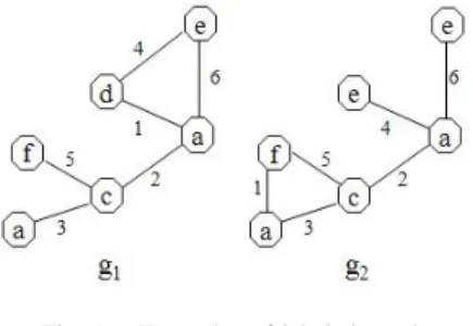
Fig. 1. Examples of labeled graph
Example 2. Let us consider the labeled graphs of Fig.1.
The sequence of edit operations those are necessary for transforming𝑔1into𝑔2is: (i) one edge deletion, (ii) one edge relabeling, (iii) one vertex relabeling, (iv) one edge insertion. By considering uniform distance measures, one can check that this sequence is the best one (i.e., the shortest). So,
𝐷𝑖𝑠𝑡𝐸𝑑(𝑔1, 𝑔2) = 4.
It is worth noticing that, in a graph database querying context, this distance measure provides information on features that both a graph of the target database and the graph query at hand disagree.
B. Mcs-Based Distance
Bunke et al. [24] have developed another kind of measure for graph similarity. It is based on the maximum common
subgraph (mcs).
Definition 9 (Similarity based on the mcs). Given two graphs 𝑔1and𝑔2, the graph similarity based on the mcs is defined as,
𝑆𝑖𝑚𝑀𝑐𝑠(𝑔1, 𝑔2) =𝑚𝑎𝑥(∣𝑔∣𝑚𝑐𝑠(𝑔11∣,∣𝑔,𝑔22)∣∣),
where ∣𝑚𝑐𝑠(𝑔1, 𝑔2)∣ denotes the number of edges in
𝑚𝑐𝑠(𝑔1, 𝑔2).
Clearly, the larger the mcs of two graphs the greater their similarity. The measure 𝑆𝑖𝑚𝑀𝑐𝑠 is normalized (i.e., 0 ≤
𝑆𝑖𝑚𝑀𝑐𝑠(𝑔1, 𝑔2) ≤ 1) since ∣𝑚𝑐𝑠(𝑔1, 𝑔2)∣ ≤ 𝑚𝑎𝑥(∣𝑔1∣ , ∣𝑔2∣). Now, the graph distance measure, 𝐷𝑖𝑠𝑡𝑀𝑐𝑠, derived from
𝑆𝑖𝑚𝑀𝑐𝑠 writes:
𝐷𝑖𝑠𝑡𝑀𝑐𝑠(𝑔1, 𝑔2) = 1 − 𝑆𝑖𝑚𝑀𝑐𝑠(𝑔1, 𝑔2) (2) Such a measure is proved to be a metric in [24] and leads to a distance in [0, 1].
The major advantage of the mcs-based approach is the fact that it does not require the use of any cost function, thereby avoiding the main drawback of edit-distance-based approach.
Example 3. Let us come back to Example 2. The
mcs-based distance measure between 𝑔1 and 𝑔2 is calculated as follows. First, the 𝑚𝑐𝑠(𝑔1, 𝑔2) is identified, see Fig. 2. Then, by applying (2), we obtain
𝐷𝑖𝑠𝑡𝑀𝑐𝑠(𝑔1, 𝑔2) = 1 −𝑚𝑎𝑥(∣𝑔∣𝑚𝑐𝑠(𝑔11∣,∣𝑔,𝑔22)∣∣) = 0.33, where ∣𝑚𝑐𝑠(𝑔1, 𝑔2)∣ = 4 and 𝑚𝑎𝑥(∣𝑔1∣ , ∣𝑔2∣) = 6.
Fig. 2. Mcs of𝑔1 and𝑔2
From a database querying point of view, this kind of similarity conveys information on the amount of features that both a graph of the queried database and a graph query agree.
C. Gu-Based Distance
Graph union(Gu)-based distance measure, introduced by
Wallis et al. [25], is based on the idea of graph union. Graph union (rather than the larger of two graphs) is used to model the size of the problem.
Definition 10 (Gu-based similarity). Given two graphs 𝑔1
and 𝑔2, the graph similarity based on graph union is defined as,
𝑆𝑖𝑚𝐺𝑢(𝑔1, 𝑔2) =∣𝑔1∣+∣𝑔∣𝑚𝑐𝑠(𝑔2∣−∣𝑚𝑐𝑠(𝑔1,𝑔2)∣1,𝑔2)∣,
where the denominator represents the size of union of the two graphs in the set theoretic sense2.
This similarity measure is also normalized and its be-haviour is somewhat close to 𝑆𝑖𝑚𝑀𝑐𝑠. It is easy to see that 𝑆𝑖𝑚𝐺𝑢(𝑔1, 𝑔2) ≤ 𝑆𝑖𝑚𝑀𝑐𝑠(𝑔1, 𝑔2) holds as well (which means that𝑆𝑖𝑚𝐺𝑢 is a stronger measure than 𝑆𝑖𝑚𝑀𝑐𝑠). The use of graph union [25] is motivated by the fact that changes in the size of the smallest graph that keep 𝑚𝑐𝑠(𝑔1, 𝑔2) constant are not taken into account in 𝑆𝑖𝑚𝑀𝑐𝑠(𝑔1, 𝑔2) whereas the measure𝑆𝑖𝑚𝐺𝑢(𝑔1, 𝑔2) does take this variation into account. The graph distance measure derived from 𝑆𝑖𝑚𝐺𝑢 can be written as:
𝐷𝑖𝑠𝑡𝐺𝑢(𝑔1, 𝑔2) = 1 − 𝑆𝑖𝑚𝐺𝑢(𝑔1, 𝑔2) (3) It was also proved to be a metric and gives values in [0, 1].
Example 4. Let us again consider the graphs provided in
Example 2. Using (3), the Gu-based distance measure between
𝑔1 and𝑔2 is
𝐷𝑖𝑠𝑡𝐺𝑢(𝑔1, 𝑔2) = 1 −∣𝑔1∣+∣𝑔∣𝑚𝑐𝑠(𝑔2∣−∣𝑚𝑐𝑠(𝑔1,𝑔2)∣1,𝑔2)∣ = 0.50, where∣𝑚𝑐𝑠(𝑔1, 𝑔2)∣ = 4 (see Example 3) and ∣𝑔1∣ = ∣𝑔2∣ = 6.
In a database querying context, this type of similarity gives also information about the number of agreements between a graph of the queried database and a graph query.
2This similarity measure looks like the Jaccard index used to measure similarity between two sets A and B, i.e.,𝐽(𝐴, 𝐵) = ∣𝐴 ∩ 𝐵∣ / ∣𝐴 ∪ 𝐵∣.
V. GRAPHSIMILARITYSKYLINE
This section is devoted to define the notion of similarity
skyline for supporting graph similarity search without the
need for specifying a global similarity measure between graph structures.
From now on, we assume that graph similarity is a com-pound notion, i.e., in order to assess similarity between graphs we consider a vector of distance measures. Each measure can be regarded as a local similarity expressing the extent to which two graphs are similar w.r.t. some features or aspects.
Definition 11 (Graph Compound Similarity, GCS). Let g
and g’ be two graphs, a graph compound similarity between
g and g’ is a vector of local distance measures denoted by 𝐺𝐶𝑆(𝑔, 𝑔′) = (𝐷𝑖𝑠𝑡1(𝑔, 𝑔′), 𝐷𝑖𝑠𝑡2(𝑔, 𝑔′), . . . , 𝐷𝑖𝑠𝑡𝑑(𝑔, 𝑔′)),
where 𝐷𝑖𝑠𝑡𝑖(𝑔, 𝑔′), for i = 1, . . ., d, stands for a local graph distance measure.
Let now 𝐷 = {𝑔1, 𝑔2, . . . , 𝑔𝑛} be a graph database and
q a graph similarity query (i.e., this means that the user is
interested in graphs of D that are the most similar to q). Since a global similarity between graphs is not available, the idea is to proceed with a d-dimensional comparison between graphs in terms of d (local) distance measures to retrieve graphs that are maximally similar in the sense of the following similarity-dominance relation.
Definition 12 (Similarity-dominance relation). Given a graph
query q and two graphs g and g’, we say that g’ is
similarity-dominated by g in the context of q, denoted by 𝑔 ≻𝑞 𝑔′, iff the following two statements hold:
1) ∀𝑖 ∈ {1, . . . , 𝑑}, 𝐷𝑖𝑠𝑡𝑖(𝑔, 𝑞) ≤ 𝐷𝑖𝑠𝑡𝑖(𝑔′, 𝑞), 2) ∃𝑘 ∈ {1, . . . , 𝑑}, 𝐷𝑖𝑠𝑡𝑘(𝑔, 𝑞) < 𝐷𝑖𝑠𝑡𝑘(𝑔′, 𝑞).
Roughly speaking, the relation𝑔 ≻𝑞𝑔′ holds if g is not less similar to q than g’ in all dimensions and (strictly) more similar to q than g’ in at least one dimension. One can observe that
g is potentially more interesting than g’ as a retrieval graph.
Therefore, the set of graphs that are the most similar to q are those that are not dominated (in the sense of Definition 12). Such graphs, called Pareto-optimal graphs, represent what we denote by the graph similarity skyline (GSS):
𝐺𝑆𝑆(𝐷, 𝑞) = {𝑔 ∈ 𝐷∣ ∕ ∃𝑔′∈ 𝐷, 𝑔′ ≻
𝑞 𝑔} (4)
where 𝑔′ ≻𝑞 𝑔 means that g is similarity-dominated by g’. To illustrate the above approach, we provide in the next section an example where d = 3. GCS(g, q) is then a vector of three components expressed by the local distance measures described in Section IV, i.e.,
𝐺𝐶𝑆(𝑔, 𝑞) = (𝐷𝑖𝑠𝑡𝐸𝑑(𝑔, 𝑞), 𝐷𝑖𝑠𝑡𝑀𝑐𝑠(𝑔, 𝑞), 𝐷𝑖𝑠𝑡𝐺𝑢(𝑔, 𝑞)).
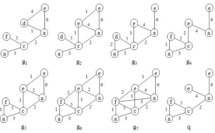
VI. ANILLUSTRATIVEEXAMPLE
Let𝐷 = {𝑔1, 𝑔2, 𝑔3, 𝑔4, 𝑔5, 𝑔6, 𝑔7} be a graph database and
q a graph similarity query, as shown in Fig. 3. In order to
provide the most interesting answers to q, one can compute the graph similarity skyline GSS(D, q). It is easy to see that
∣𝑔1∣ = 6, ∣𝑔2∣ = 7, ∣𝑔3∣ = 7, ∣𝑔4∣ = 6, ∣𝑔5∣ = 8, ∣𝑔6∣ =9, ∣𝑔7∣ =
Fig. 3. The graph database D and the graph query q
10 and∣𝑞∣ = 6. Table 2 summarizes the values of ∣𝑚𝑐𝑠(𝑔𝑖, 𝑞)∣, for i = 1,. . .,7. TABLE II INFORMATIONABOUT∣𝑀𝑐𝑠(𝑔𝑖, 𝑞)∣ ∣𝑀𝑐𝑠(𝑔𝑖, 𝑞)∣ (𝑔1, 𝑞) 4 (𝑔2, 𝑞) 4 (𝑔3, 𝑞) 4 (𝑔4, 𝑞) 3 (𝑔5, 𝑞) 5 (𝑔6, 𝑞) 5 (𝑔7, 𝑞) 6 TABLE III DISTANCEMEASURES 𝐷𝑖𝑠𝑡𝐸𝑑(𝑔𝑖, 𝑞) 𝐷𝑖𝑠𝑡𝑀𝑐𝑠(𝑔𝑖, 𝑞) 𝐷𝑖𝑠𝑡𝐺𝑢(𝑔𝑖, 𝑞) (𝑔1, q) 4 0.33 0.50 (𝑔2, q) 4 0.43 0.56 (𝑔3, q) 3 0.43 0.56 (𝑔4, q) 2 0.50 0.67 (𝑔5, q) 3 0.38 0.44 (𝑔6, q) 4 0.44 0.50 (𝑔7, q) 4 0.40 0.40
Now the graph similarity vectors𝐺𝐶𝑆(𝑔𝑖, 𝑞), for i = 1,. . .,7, are shown in Table III. By applying (4), the set of Pareto optimal graphs, i.e. the graph similarity skyline, is given by
𝐺𝑆𝑆(𝐷, 𝑞) = {𝑔1, 𝑔4, 𝑔5, 𝑔7}.
One can easily check that𝑔2(resp.𝑔3) /∈ 𝐺𝑆𝑆(𝐷, 𝑞) since it is dominated by𝑔7 (resp.𝑔5) and𝑔6 /∈ 𝐺𝑆𝑆(𝐷, 𝑞) since it is dominated by𝑔1. Thus, the graphs of𝐷 that are maximally similar to q are𝑔1,𝑔4,𝑔5 and𝑔7. Indeed,
∙ Graph 𝑔1 is the most interesting w.r.t. the measure
𝐷𝑖𝑠𝑡𝑀𝑐𝑠. This is due to the two following reasons: i) 𝑔1 satisfies a maximum number of features required by
𝑞 than other graphs with the same size; ii) 𝑔1 and𝑞 are of the same size. But, 𝑔1 is the less interesting w.r.t. to superfluous and missing features.
∙ Graph 𝑔4 is the best w.r.t. the measure 𝐷𝑖𝑠𝑡𝐸𝑑. This means that it is the most interesting w.r.t. to the numbers of disagreements with 𝑞. On the other hand, 𝑔4 is much less satisfactory w.r.t. to the agreements with 𝑞 in the sense of the mcs notion.
∙ Graph 𝑔7 is the most interesting w.r.t. the measure
𝐷𝑖𝑠𝑡𝐺𝑢. This is due to the fact that 𝑔7 ⊃ 𝑞. But, it is the less interesting w.r.t. a superfluous feature-based criterion.
∙ Graph 𝑔5 may be a good compromise between the three measures𝐷𝑖𝑠𝑡𝐸𝑑,𝐷𝑖𝑠𝑡𝑀𝑐𝑠and𝐷𝑖𝑠𝑡𝐺𝑢.
Let us now take a look at the results obtained when using only a single similarity measure between graphs. If we are interested in the best𝑘 (= 3) answers, 𝑔3 is then returned for instance by the edit-distance-based approach as answer to the user, but with the skyline-based approach 𝑔3 is not returned as answer since𝑔5 does better than it.
VII. REFININGGRAPHSIMILARITYSKYLINE
One of the problems that may arise when computing the set GSS (and a skyline in general) is its size which is often quite large. From a user point of view, it is very desirable to have a suitable criterion to select a small interesting subset of graphs of the skyline GSS. One solution is to use the criterion of diversity [26] to select a subset of graphs which is as diverse
as possible and then provide the user with a picture of the
whole set GSS.
Let S be a subset of GSS. The diversity of S means that the graphs it includes should be dissimilar amongst each other. The goal is to extract from GSS a subset 𝕊 of size k (a user-defined parameter) with a maximal diversity. Adapted from [27], the proposed approach defines the diversity of S (⊆ 𝐺𝑆𝑆) of size k by a vector 𝐷𝑖𝑣(𝑆) = (𝑣1, 𝑣2, 𝑣3) such as
𝑣𝑖 = 𝑚𝑖𝑛{𝐷𝑖𝑠𝑡𝑖(𝑔, 𝑔′)∣𝑔, 𝑔′ ∈ 𝑆},
where 𝐷𝑖𝑠𝑡1 = 𝐷𝑖𝑠𝑡𝑁−𝐸𝑑 (the normalized version of the distance 𝐷𝑖𝑠𝑡𝐸𝑑 obtained using the function f(x) = x/(1+x)),
𝐷𝑖𝑠𝑡2 = 𝐷𝑖𝑠𝑡𝑀𝑐𝑠 and 𝐷𝑖𝑠𝑡3 = 𝐷𝑖𝑠𝑡𝐺𝑢. The value 𝑣𝑖
expresses the diversity in the𝑖𝑡ℎ dimension of the subset S. To identify the subset𝕊 of interest, we consider all subsets
𝑆 ⊆ 𝐺𝑆𝑆 with ∣𝑆∣ = 𝑘 (i.e., the size of 𝑆 is 𝑘) as candidates
and apply the following steps:
Step 1. For each dimension i (i = 1,. . .,3), rank-order all
candidates subsets S in decreasing way according to their diversity 𝑣𝑖 in that dimension. Let 𝑟𝑎𝑛𝑘𝑖(𝑆) be the rank of S w.r.t.𝑖𝑡ℎ dimension. Rank value 1 means the best diversity value and rank value M means the worst diversity value (M is the number of subsets of size k of the set GSS).
Step 2. Evaluate a candidate S by:
𝑣𝑎𝑙(𝑆) =∑𝑖=1,...,3𝑟𝑎𝑛𝑘𝑖(𝑆).
The subset that minimizes this criterion (i.e., minimizes the sum of its positions in all ranks) is considered as a subset with a maximal diversity. So, 𝕊 is characterized by
where 𝑆 ⊆ 𝐺𝑆𝑆 and ∣𝑆∣ = 𝑘.
Example 5. Let us come back to the example given in
section VI, where𝐺𝑆𝑆(𝐷, 𝑞) = {𝑔1, 𝑔4, 𝑔5, 𝑔7}. Assume now that the user is interested in the best k (= 2) graphs w.r.t. the diversity criterion. One can easily check that the set of all candidates contains 6 subsets of size k, see Table IV.
TABLE IV
CANDIDATES WITHTHEIRDIVERSITY
𝑣1 𝑣2 𝑣3 𝑆1= {𝑔1, 𝑔4} 0.86 0.67 0.80 𝑆2= {𝑔1, 𝑔5} 0.83 0.50 0.60 𝑆3= {𝑔1, 𝑔7} 0.87 0.60 0.67 𝑆4= {𝑔4, 𝑔5} 0.80 0.62 0.73 𝑆5= {𝑔4, 𝑔7} 0.83 0.70 0.77 𝑆6= {𝑔5, 𝑔7} 0.75 0.50 0.61
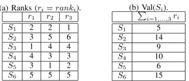
Now, steps 1 and 2 lead to the results depicted in Table V.
TABLE V EVALUATION OFALLCANDIDATES. (a) Ranks (𝑟𝑖= 𝑟𝑎𝑛𝑘𝑖). 𝑟1 𝑟2 𝑟3 𝑆1 2 2 1 𝑆2 3 5 6 𝑆3 1 4 4 𝑆4 4 3 3 𝑆5 3 1 2 𝑆6 5 5 5 (b) Val(∑ 𝑆𝑖). 𝑖=1,...,3𝑟𝑖 𝑆1 5 𝑆2 14 𝑆3 9 𝑆4 10 𝑆5 6 𝑆6 15
From Table V-(b), one can easily see that 𝑣𝑎𝑙(𝑆1) is the minimal value. So,𝕊 = 𝑆1= {𝑔1, 𝑔4}.
VIII. CONCLUSION
In this paper, we have proposed an alternative approach to support graph similarity search. The key concept of this approach is the notion of graph similarity skyline we intro-duced. This kind of skyline allows retrieving all graphs of the queried database that are not dominated in the sense of the similarity-dominance relation defined. Namely, graphs those are maximally-similar to the graph query at hand. Each answer graph is provided to the user with a vector of scores showing different similarities pertaining to different features. We have also shown how to select a maximally diverse subset of a graph similarity skyline.
We plan to conduct some experiments on real-life data to demonstrate the effectiveness and efficiency of the approach. To this end, a system implementing it is underway.
ACKNOWLEDGMENTS
This work was supported in part by the National Agency for Research under project AOC on the reference ANR-08-CORD-009, and Brittany region.
REFERENCES
[1] Y. Tian, R. McEachin, C. Santos, D. J. States, and J. M. Patel, “Saga: a subgaph matching tool for biological graphs,” Bioinformatics, vol. 23(2), pp. 232–239, 2007.
[2] H. Hu, Y. Hang, J. Han, and X. Zhou, “Mining coherent dense subgraphs across massive biological network for fonctional discovery,” Bioinfor-matics, vol. 1(1), pp. 1–9, 2005.
[3] D. Conte, P. Foggia, C. Sansone, and M. Vento, “Thirty years of graph matching in pattern recognition,” Inter. J. of Pattern Recogn. and Art. Intell., vol. 18 (3), pp. 265–298, 2004.
[4] N. Zhang, T. Ozsu, I. Ilyas, and A. Aboulnaga, “Fix: eature-based indexing technique for xml documents,” in Proc. of VLDB, 2006, pp. 259–270.
[5] S. Klinger and J. Austin, “Chemical similarity searching using a neural graph matcher,” in Proc. of ESANN, 2005, pp. 479–484.
[6] D. Cai, Z. Shao, X. He, X. Yan, and J. Han, “Community mining from multirelational networks,” in Proc. of PPKDD, 2005, pp. 445–452. [7] Z. Zeng, A. Tung, J. Wang, J. Feng, and L. Zhou, “Comparing stars: On
approximating graph edit distance,” in Proc. of VLDB, 2009, pp. 25–36. [8] C. Chen, X. Yan, P. S. Yu, J. Han, D.-Q. Zhang, and X. Gu, “Towards Graph Containment Search and Indexing,” in Proc. of VLDB, Vienna, Austria, sept 23-27 2007, pp. 926–937.
[9] X. Yan, P. S. Yu, and J. Han, “Graph indexing: A frequent structurebased approach,” in Proc. of ACM SIGMOD, 2004, pp. 335–346.
[10] S. Zhang, J. Z. Li, H. Gao, and Z. Zou, “A novel approach for efficient supergraph query processing on graph databases,” in Proc. of EDBT, march 24-26 2009, pp. 204–215.
[11] S. Zhang, M. Hu, and J. Yang, “Treepi: A novel graph indexing method,” in Proc. of ICDE, 2007, pp. 966–975.
[12] Y. Tian and J. M. Patel, “Tale : A tool for approximate large graph matching,” in Proc. of ICDE, Cancun, Mexico, 2008, pp. 963–972. [13] E. Petrakis and C. Faloutsos, “Similarity searching in medical image
databases,” Proc. of TKDE, vol. 9 (3), pp. 435 –447, May 1997. [14] X. Yan, P. S. Yu, and J. Han, “Substructure similarity search in graph
databases,” in Proc. of ACM SIGMOD, 2005, pp. 766–777.
[15] H. He and A. K. Singh, “Closure-tree: An index structure for graph queries,” in Proc. of ICDE, 2006, pp. 38–52.
[16] H. Shang, K. Zhu, X. Lin, Y. Zhang, and R. Ichise, “Similarity search on supergraph containment,” in Proc. of ICDE, march 1-6 2010, pp. 637–648.
[17] S. Borzsonyi, D. Kossmann, and K. Stocker, “The skyline operator,” in Proc. of ICDE, 2001, pp. 421–430.
[18] J. Pei, B. Jiang, X. Lin, and Y. Yuan, “Probabilistic skylines on uncertain data,” in Proc. of VLDB, 2007, pp. 15–26.
[19] M. L. Yiu and N. Mamoulis, “Efficient processing of top-k dominating queries on multi-dimensional data,” in Proc. of VLDB, 2007, pp. 483– 494.
[20] M. E. Khalefa, M. F. Mokbel, and J. J. Levandoski, “Skyline query processing for incomplete data,” in Proc. of ICDE, 2008, pp. 556–565. [21] A. Hadjali, O. Pivert, and H. Prade, “Possibilistic contextual skylines with incomplete preferences,” in Proc. of SoCPaR, Cergy Pontoise, Paris, France, December 07-10, 2010.
[22] L. Zou, L. Chen, M. T. Ozsu, and D. Zhao, “Dynamic skyline queries in large graphs,” in Proc. of DASFAA, 2010, pp. 62–78.
[23] H. Bunke, “On a relation between graph edit distance and maximum common subgraph,” Pattern Recogn. Letters, vol. 18 (9), pp. 689–697, August 1997.
[24] H. Bunke and K. Shearer, “A graph distance metric based on the maximal common subgraph,” Pattern Recogn. Letters, vol. 19 (3-4), pp. 255–259, March 1998.
[25] W. D. Wallis, P. Shoubridge, M. Kraetz, and D. Ray, “Graph distances using graph union,” Pattern Recogn. Letters, vol. 22 (6-7), pp. 701–704, May 2001.
[26] D. McSherry, “Diversity-conscious retrieval,” in Proc. of ECCBR. Springer-Verlag, 2002, pp. 219–233.
[27] S. Kukkonen and J. Lampinen, “Ranking-dominance and many-objective optimization,” in IEEE Congress on Evolutionary Computation, 2007, pp. 3983–3990.