HAL Id: hal-01870459
https://hal.archives-ouvertes.fr/hal-01870459
Submitted on 7 Sep 2018
HAL is a multi-disciplinary open access
archive for the deposit and dissemination of
sci-entific research documents, whether they are
pub-lished or not. The documents may come from
teaching and research institutions in France or
abroad, or from public or private research centers.
L’archive ouverte pluridisciplinaire HAL, est
destinée au dépôt et à la diffusion de documents
scientifiques de niveau recherche, publiés ou non,
émanant des établissements d’enseignement et de
recherche français ou étrangers, des laboratoires
publics ou privés.
Arturo Gonzalez, Franziska Schmidt
To cite this version:
Arturo Gonzalez, Franziska Schmidt.
Effects on bridges of the various vehicle configurations.
[Research Report] IFSTTAR - Institut Français des Sciences et Technologies des Transports, de
l’Aménagement et des Réseaux. 2017, 58 p. �hal-01870459�
DELIVERABLE REPORT
DELIVERABLE N0: D5.2 DISSEMINATION LEVEL: PUBLICTITLE: EFFECTS ON BRIDGES OF THE VARIOUS VEHICLE CONFIGURATIONS
DATE: 01/01/2017
VERSION: DRAFT
AUTHOR(S): ARTURO GONZALEZ (UCD)
FRANZISKA SCHMIDT (IFSTTAR)
REVIEWED BY: BERNARD JACOB (IFSTTAR)
APPROVED BY: COORDINATOR – PAUL ADAMS (VOLVO)
GRANT AGREEMENT N0: 605170
PROJECT TYPE: THEME 7 TRANSPORT – SST GC.SST.2012.1-5: INTEGRATION AND OPTIMISATION OF RANGE EXTENDERS ON ELECTRIC VEHICLES
PROJECT ACRONYM: TRANSFORMERS
PROJECT TITLE: CONFIGURABLE AND ADAPTABLE TRUCKS AND TRAILERS FOR OPTIMAL TRANSPORT EFFICIENCY
PROJECT START DATE: 01/09/2013
PROJECT WEBSITE: WWW.TRANSFORMERS-PROJECT.EU
COORDINATION: VOLVO (SE)
Executive summary
This deliverable D5.2 assesses the impact of the TRANSFORMERS solutions on bridges, as far as the static and dynamic vertical effects are concerned. The static effect has been assessed in terms of extreme effects and fatigue, and the dynamic effects have been evaluated in terms of interaction with the bridge.
As far as these two impacts are concerned, the sensitive parts of the infrastructure have been chosen, independently for the static and the dynamic behaviour of bridges.
For the static effect on bridges, simply supported, single span and continuous 2-span bridges with spans of length 10 meters, 20 meters, 30 meters and 50 meters have been chosen, while the considered effects are the bending moment at mid-span and the shear force at the supports. Literature has shown that these are the sensitive infrastructure elements as far as the static effect of traffic on bridges is concerned.
For the dynamic effect on bridges, a simply supported bridge with span lengths 10m, 15m and 20m is used for simplified assessment. For the detailed assessment, a solid slab plate deck model is used to represent a bridge with a cross section of inverted T-beams and several span lengths (9, 11, 13, 15, 17, 19, 21 meters). Here again, these are the infrastructure elements that have been highlighted as sensitive and to be assessed.
The second step has been to define the truck configurations to assess: until details of the TRANSFORMERS solution were available, standard truck models were chosen, namely the conventional 40t-semi-trailer, a 41t-semi-trailer, a 44t semi-trailer and a 38t- truck-trailer with 2 axles. Then, with the finalizing of the TRANSFORMERS solution, the truck models have been refined in order to compare the effects of the truck + Hybrid on Demand (HoD) trailer combination and the effects of the truck + load optimization trailer.
For all these truck configurations, the effect on bridges has been assessed and compared.
When considering the 40t semi-trailer as reference (impact on bridge normalized to 1.0), the extreme static effect of the chosen truck configurations varies between 0.93 (38T vehicle) and 1.33 (44T vehicle).
Similarly, when considering the 40t semi-trailer as reference (lifetime of bridge normalized to 100 years), the lifetime of bridges in good shape and under the sole assumption of static effect of the fully loaded TRANSFORMERS configurations varies between 89 and 136 years.
For the dynamic effect on bridge, one can notice that for the bridge scenarios with stochastic road profiles being investigated, changes in values of dynamic amplification factor (usually called “DAF” in the literature, but called “DAmF” hereafter to avoid confusing with the TRANSFORMERS partner and OEM DAF) associated to the node location holding the largest static bending moment has hardly been altered with the truck configurations under investigation. Only when the truck has increased (44t) or decreased (38t) in GVW noticeably, DAmF of the bridge response has shown to be affected.
Contents
1 Introduction ... 5
2 The truck models ... 6
2.1 First truck configurations ... 6
2.2 TRANSFORMERS Truck: Volvo tractor and SCB hybrid trailer/Van Eck trailer ... 7
2.3 Dynamic parameters ... 8
3 Static effects and fatigue damage of the given configurations of trucks ... 10
3.1 Methodology for effect assessment ... 10
3.1.1 Comparison of extreme effects ... 10
3.1.2 Comparison of fatigue life ... 10
3.2 Infrastructure choice ... 11
3.3 Comparison of extreme effects ... 13
3.4 Comparison of fatigue life ... 14
4 Dynamic effects of the given configurations of trucks ... 17
4.1 Introduction ... 17
4.2 Methods of assessment ... 17
4.2.1 Simple method using a vehicle modeled as a series of constant forces moving on a planar bridge model ... 18
4.2.2 Complex method using a 3D vehicle-bridge interaction model. ... 21
4.3 Choice of structure/infrastructure ... 23
4.3.1 The bridge model ... 23
4.3.2 The road profile... 24
4.4 Simple assessment ... 25
4.4.1 Definition of parameters ... 26
4.4.2 Results of simple assessment ... 27
4.4.3 Results for Truck Type A ... 27
4.4.4 Results for Truck Type B ... 28
4.4.5 Results for Truck Type C ... 30
4.4.6 Preliminary conclusions ... 31
4.5 Detailed assessment ... 31
4.5.1 Truck case 0-a (EU reference truck – 40 t) ... 33
4.5.2 Truck Case 0-b (extra tonne in tractor – 41 t) ... 35
4.5.3 Truck Case 0-c (44 t) ... 37
4.5.4 Truck Case 0-d (38 t) ... 39
4.5.5 Truck Case 1 (extra tonne in trailer – 41 t) ... 41
4.5.6 Truck Case 2 (Transformers configuration – 40 t) ... 43
4.5.7 Truck Case 3 (Transformers configuration – 41 t) ... 45
4.6 Summary ... 46
5 Conclusions ... 49
6 References ... 50
7 Acknowledgment ... 52
8.1 Ratio of static extreme effects for the chosen infrastructure types ... 53 8.2 Fatigue life for the various bridge configurations ... 55
1 Introduction
This deliverable D5.2 of the FP7 project TRANSFORMERS deals with the effects on bridges of vehicle configurations that have been designed in other work packages of the project. For that, two first steps have been 1/ to define the infrastructure parts to be assessed, and 2/ to define precisely the chosen vehicle configurations to be able to evaluate the impact.
Indeed, the objective is to assess the static and the dynamic effect of the TRANSFORMERS solution on bridges. This effect depends on:
1. The bridge structure: number of spans, length of spans, type of supports… 2. The effect of the bridge: bending moment, shear force …
3. The point of interest of the bridge structure: mid-span, supports …
Consequently, the first step has been to define the parts of the bridge infrastructure to be assessed, for the static effect (Section 3.2) and for the dynamic effect (Section 4). This means that the way of assessing the effect has also been chosen for all these infrastructure elements (see Section 3.1 for the methods of assessing the static effect).
After knowing the type of infrastructure to assess and the involved methods, the vehicle configurations to be considered had to be defined. This has been done twice during the TRANSFORMERS project:
1. Once before the definition of the TRANSFORMERS solution: as at that time the TRANSFORMERS vehicle had not been designed or built yet, calculations of the effects of simplified vehicles have been done in order to have a first overview on the comparative effects between a conventional 40t-vehicle and a 41t-truck that would have integrated the extra 1t for the electrical engine.
2. The vehicle configurations have been defined precisely after the design of the TRANSFORMERS solution. This has been done by collaboration with other packages (namely WP1 and WP4). The definition of these vehicle configurations is given here in Section 2, before the explanations and results of the static and dynamic calculations as the truck models are the same for both types of calculations.
The static effect of the truck configurations on bridges in explained in Section 3, Section 4 explains the computations of the dynamic effect of the truck configurations on bridges.
2 The truck models
These truck models are the same for all WP5 deliverables.
The characteristics of the vehicle configurations to assess have been defined, in terms of dimensions, axle loads, and axle stiffness’s. This has first been the case for simplified vehicle configurations, as the TRANSFORMERS solution was not available then. These simplified configurations are the 40t-reference truck, a 41t semi-trailer, a 44t ton semi-trailer and a 38t semi-trailer, as detailed in Section 2.1.
Then, when the TRANSFORMERS solution has been designed, these vehicles configurations have been detailed: the configurations to assess have been chosen as the Volvo truck with hybrid-on-demand trailer and the Volvo truck with movable roof trailer (Section 2.2). The same combinations with DAmF truck are not shown here as the effects on bridges are quite similar.
2.1 First truck configurations
The axle spacing is the same for all three trucks and provided in Figure 1. The axle weight distribution of the three trucks is provided in Table 1.
Figure 1: Axle spacing for typical European truck configuration
These axle weights have been chosen by using the reference 40t, conventional European semi-trailer (called “Truck type A” in Table 1) and by adding 1 tonne as the Directive 2015/719 allows it for power trains that reduce pollution. Trucks B and C therefore corresponds to different assumptions on axle repartition of this 1 extra tonne.
Table 1: Truck configurations tested in Section on “Simple assessment”
Truck
type Number axles
Weight on axles (t) Distance from 1st axle (m) Axle
1 Axle 2 Axle 3 Axle 4 Axle 5 Axle 1 Axle 2 Axle 3 Axle 4 Axle 5
A 5 6.5 11 7.5 7.5 7.5 0 3.6 9.93 11.24 12.55
B 5 6.5 11.16 8.34 7.5 7.5 0 3.6 9.93 11.24 12.55
2.2 TRANSFORMERS Truck: Volvo tractor and SCB hybrid trailer/Van Eck
trailer
As the TRANSFORMERS solutions have been defined, the vehicle configurations have been detailed. The static mechanical properties of axle spacing and weight distribution (new and typical configurations for comparison purposes) of the trucks employed in the following sections are shown in Table 2 and Table 3 respectively. Distances provided in Table 2 are measured in meters with respect to axle 1:
Five of these vehicles have the same axle spacings, which are adopted as the EU reference truck: ‘Case 0-a’, ‘Case 0-b’, ‘Case 0-c’, ‘Case 0-d’ and ‘Case 1’. The latter only vary in the weight distribution.
o Case 0-a corresponds to the reference vehicle (40t, European conventional semi-trailer),
o Case 0-b corresponds to a 41t semi-trailer, obtained from case 0-a by adding 1t on the truck (0.5t on the first axle and 0.5t on the second axle),
o Case 0-c is a 44t semi-trailer, as it is allowed in many European countries now, o Case 0-d is a 38t semi-trailer (used in the European standards of safety barriers),
The vehicle “TRANSFORMERS truck + HoD trailer” corresponds to the TRANSFORMERS truck that has been chosen in the frame of the TRANSFORMERS solution with the HoD trailer built by SCB. The values of axle loads have been obtained from WP4 partners.
The vehicle “TRANSFORMERS truck + movable roof trailer” corresponds to the TRANSFORMERS truck that has been chosen in the frame of the TRANSFORMERS solution with the movable roof trailer built by Van Eck. The values of axle loads have been obtained from WP4 partners.
Truck labeled ‘Case1’ corresponds to Truck type B of the detailed assessment (added here for comparison sake),
Trucks labeled ‘Case 2’ and ‘Case 3’ are new Transformers trucks with different axle spacing. There TRANSFORMERS solutions correspond
Axle weights along with the Global Vehicle Weight (GVW) in tonnes for all 9 vehicles being tested are given in Table 3.
Table 2. Axle spacings employed in Section 5 “Detailed assessment”
Distances (m) Axle 1 to axle
2 Axle 1 to axle 3 Axle 1 to axle 4 Axle 1 to axle 5
Case 0-a 3.6 9.93 11.24 12.55 Case 0-b 3.6 9.93 11.24 12.55 Case 0-c 3.6 9.93 11.24 12.55 Case 0-d 3.6 9.93 11.24 12.55 Case 1 3.6 9.93 11.24 12.55 Case 2 3.8 9.72 11.03 12.34 Case 3 3.8 9.72 11.03 12.34
Table 3. Axles weights employed in Section 5 “Detailed assessment”
Weights in
tonnes GVW Axle 1 Axle 2 Axle 3 Axle 4 Axle 5
Case 0-a 40 6.5 11 7.5 7.5 7.5 Case 0-b 41 7.0 11.5 7.5 7.5 7.5 Case 0-c 44 6.5 11 8.8333 8.8333 8.8333 Case 0-d 38 6.5 11 6.8333 6.8333 6.8333 TRANSFORMERS truck + HoD trailer 41 6.577 11.57 7.77 7.77 7.77 TRANSFORMERS truck + movable roof trailer 40 6.577 11 7.58 7.58 7.58
Case 1 41 6.5 11.16 8.34 7.5 7.5
Case 2 40 6.9348 10.8224 7.4144 7.4144 7.4144
Case 3 41 6.934 10.822 7.748 7.748 7.748
2.3 Dynamic parameters
For the assessment of the static effect and for the simple assessment of dynamic effect (Section 4.2.1), only the static mechanical parameters of the truck described in the previous subsection are necessary. However, values of dynamic parameters must be adopted for a full vehicle-bridge interaction (VBI) simulation. The vehicle model is based on a typical 5-axle articulated truck. Two significant bodies can be distinguished, tractor and semi-trailer, which are represented by lumped body masses, ms and mT, in Figure 2. Each of the axles is modelled as a rigid bar with lumped masses
that represent the total mass of the wheel and suspension assemblies. The body masses are linked to lumped axle masses via spring-dashpot systems simulating the suspension. Spring-dashpot systems that denote the tyres are used to connect the axle masses to the road surface. In total, the model has 15 degrees of freedom (DOFs). This model is assumed to have negligible lateral and yaw movements. Table 4 provides the mechanical properties of the vehicle, based on the work by Cantero et al (2009, 2010). These are typical numerical values for these parameters.
(a) (b)
Figure 2. Five-axle articulated vehicle dynamic model: (a) Side view, (b) Front
Table 4. Vehicle properties (subscripts R and L refer to Right and left axle respectively)
Mass data
Tractor front axle: kg 700
Tractor rear axle: kg 1000
Semitrailer axles: kg 800
Spring rates: kN/m (suspensions)
K1R, K1L 200
K2R, K2L 500
K3-5R, K3-5L 375
Spring rates: kN/m (tyre)
Kt1R, Kt1L 875
Kt2R, Kt2L 1750
Kt3-5R, Kt3-5L 1750
Viscous damping rates: kNs/m (suspensions)
C1-5R, C1-5L 5
Viscous damping rates: kNs/m (Tyre)
3 Static effects and fatigue damage of the given
configurations of trucks
In this chapter, the methodology for static vertical effect assessment is explained. This corresponds to the effect that a vertical moving load would exert on the structure when moving very slowly on the deck. Two phenomenons can then be studied: the extreme effects which mean the extreme effect the bridge has to support during the passing of the moving load, and the fatigue life which corresponds to the lifetime of the structure under the assumption of passing of the vehicle configurations under consideration.
The methodology used here is the same as the one that has been used in the studies on longer and/or heavier trucks for the EU (Transport and Mobility Leuven, 2008) or (Vrouwenvelder, 2008). The following chapter is organized as follows: Section 3.1 explains the methodology for assessment, then section 3.2 lists the infrastructure for which this assessment will be done. The results are given in Section 3.3 for the extreme effects and Section 3.4 for the fatigue life.
3.1 Methodology for effect assessment
The effect on a moving load is given by the convolution of the moving load with the influence line of the effect. In particular, a moving vehicle with N axles would be considered as N moving loads, with given axle loads and given distance between the axles.
If is the value of the influence line of effect at coordinate and we consider truck , the global effect at coordinate x is given by the sum of the effects of all axles:
Where:
is the axle load on axle of truck ,
is the distance between axle 1 and axle for truck (so by definition, ).
The values of and are given by the vehicle configurations (Section 2) and the function is representative of the chosen infrastructure (Section 3.2).
3.1.1 Comparison of extreme effects
By computing this effect , its maximum value can be assessed for the various vehicle configurations. Two vehicle configurations can then be compared in terms of extreme effects by calculating the ratio of the effect .
More precisely, in this work where we compare the “new” vehicles (TRANSFORMERS solution) to the 40t-reference truck, this means that the ratio of interest will be for each vehicle:
Where:
depends on the type of effect and the vehicle ,
is the maximum effect of vehicle ,
is the maximum effect of the reference vehicle (40t conventional trailer). One can notice that by definition, for all effects, ,
3.1.2 Comparison of fatigue life
Fatigue is a well-known issue for steel bridges, or steel elements in composite bridges. It is the progressive and localized structural damage that occurs when a material is subjected to cyclic loading. Therefore, it is linked to the GVW of the vehicles, but also the axle loads.
The fatigue life of the structure is given by the stress cycles exerted by the moving load on the structure. The aggressivity of the vehicle configurations is given by the following equations, that correspond to the S-N Woehler curves (Figure 3):
Where:
is the stress cycle exerted by the moving load (vehicle) on the chosen infrastructure,
is the fatigue limit (depends of the material of the structure and given in Eurocode 3 and standards),
Figure 3: S-N Woehler curves (extracted for EN1993).
We make here the assumption that the cycles exerted by the reference truck on the structure are equal to the endurance limit:
So, with Miner’s rule, the fatigue life on the structure can be assessed through: Where:
is the agressivity of the vehicle,
Lifetime of the structure is given by: .
3.2 Infrastructure choice
The effect of the moving load of the vehicle of the structure is calculated with means of influence lines: an influence line of a given effect (bending moment, stress stress, …) is the effect caused by a unit load moving along the structure.
In order to take into account the various possibilities of bridges structures, it has been decided to use “theoretical” influence lines, and not influence lines of effects of existing, well-known bridges.
Therefore, two types of structures have been chosen:
Simply supported, single span bridge,
Two-span, simply supported bridges (continuous over the central support), with both spans of equal length.
These types of structures are common and numerous on European roads (Figure 4).
Figure 4: Simply supported, single span bridge (left) and simply supported, two-span bridge (right).
For each one of these structures, several span lengths have been chosen, namely 10 meters, 20 meters, 30 meters and 50 meters. Indeed:
Spans smaller than 10 meters are not assessed here as only one axle or one axle group could be at a given time on the structure; therefore assessing the effect of the whole truck could not be possible.
Spans greater as 50 meters are not sensitive to single-vehicle-effects.
For each of these structures, several effects will be investigated: bending moment at mid-span and shear force at support.
Therefore the computations that have been done can be summarized with:
Table 5: List of computations
Type of structure Span length Effect
Simply supported, single span
10 m Shear force at support 0 Moment at mid-span 1 20 m Moment at mid-span 1
Shear force at support 0 30 m Shear force at support 0 Moment at mid-span 1 50 m Shear force at support 0 Moment at mid-span 1
2-span, simply supported bridge (continuous over the
central support)
10 m
Shear force at support 0 Bending moment at mid-span 1
Shear force at support 1 (intermediate support) 20 m
Shear force at support 0 Bending moment at mid-span 1
Shear force at support 1 (intermediate support) 30 m
Shear force at support 0 Bending moment at mid-span 1
Shear force at support 1 (intermediate support) 50 m
Shear force at support 0 Bending moment at mid-span 1
Shear force at support 1 (intermediate support)
The influence lines for these infrastructure elements are represented on Figure 5 and Figure 6.
Figure 5: Influence lines for simply supported, single span bridge (here, the Figure is given
0 0,5 1 1,5 2 2,5 3 0 5 10 15 Shear on support 0 Moment at mid-span 1
Figure 6: Influence lines for simply supported, 2-span bridge (here, the Figure is given for span length of 10 meters).
3.3 Comparison of extreme effects
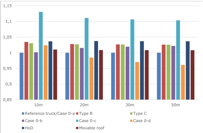
When applying the methodology explained above, the extreme effects of the bending moment at mid-span, of the simply supported, single span bridge can be compared, see Figure 7: one can see that Case 0-c (44t-semi trailer) has the highest agressivity. When comparing the HoD TRANSFORMERS solution and the movable roof solution, the first one is the most aggressive: This means that on a given bridge and for a given effect, the amplitude (highest value) of the effect caused by the HoD TRANSFORMERS solution is bigger than the one caused by the movable roof solution.
Figure 7: Ratio of extreme bending moment on the simply supported, single span bridge, for various length of span and the various vehicle configurations.
The situation is the same and even clearer when considering the shear force at support 0 for the same simply supported, single span bridge, see Figure 8: Case 0-c is by far the most aggressive vehicle configuration. Moreover, from the two TRANSFORMERS configurations, the HoD alternative is the most aggressive.
-1,5 -1 -0,5 0 0,5 1 1,5 2 2,5 0 5 10 15 20 25 Moment at mid-span 1 Moment on support 1 0 0,2 0,4 0,6 0,8 1 1,2 10m 20m 30m 50m
Reference truck/Case 0-a Type B Type C
Case 0-b Case 0-c Case 0-d
Figure 8: Ratio of extreme shear force at support 0 on the simply supported, single span bridge, for various length of span and the various vehicle configurations.
The conclusions are similar for the other bridge configurations. The whole results can be found in Appendix 8.1.
3.4 Comparison of fatigue life
Here the lifetime of the structure is calculated by comparing the effect caused by traffic that would be composed only by one type of vehicle.
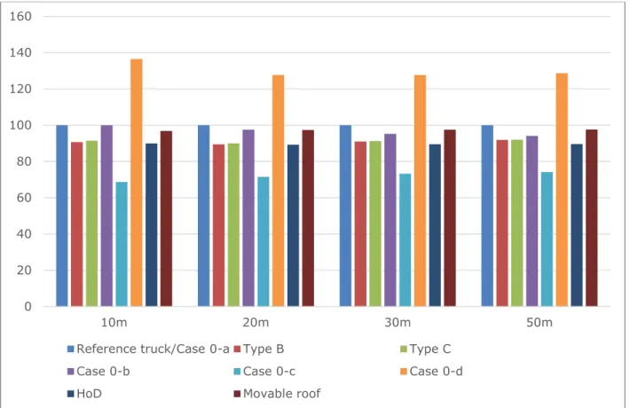
Consequently, the fatigue life is computed as being minimal for Case 0-c. Types B and C have similar fatigue life, see Figure 9 and Figure 10.
The conclusions are similar for all effects and bridge configurations that have been chosen, see Appendix 8.2.
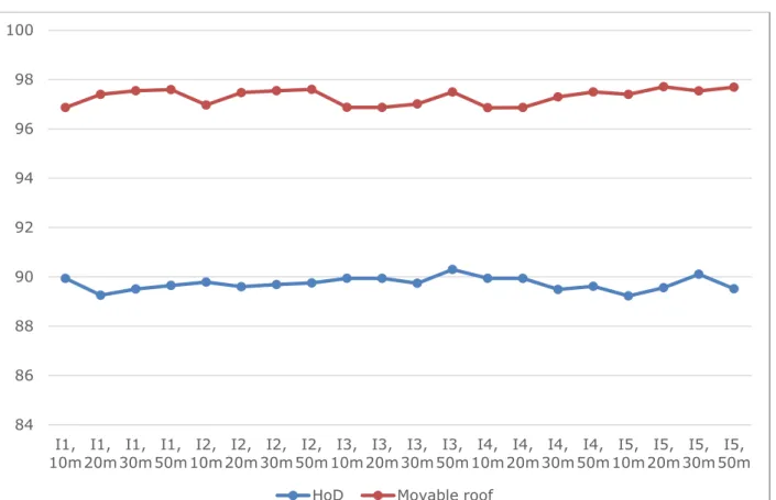
The two TRANSFORMERS solutions (HoD and movable roof) induce similar fatigue life, reduced when compared to the one induced by the 40t reference vehicle. More precisely, The solution “TRANSFORMERS truck + HoD trailer” induces a approximately a 10%-reduction of the lifetime of the bridge, whereas the combination “TRANSFORMERS truck + movable roof” induces a 3% reduction, see Figure 11. 0,85 0,9 0,95 1 1,05 1,1 1,15 10m 20m 30m 50m
Reference truck/Case 0-a Type B Type C
Case 0-b Case 0-c Case 0-d
Figure 9: Fatigue life by considering the bending moment at mid-span for the simply supported, single span bridge.
Figure 10: Fatigue life by considering the shear force at support 0 for the simply supported, single span bridge.
0 20 40 60 80 100 120 140 10m 20m 30m 50m
Reference truck/Case 0-a Type B Type C
Case 0-b Case 0-c Case 0-d
HoD Movable roof
0 20 40 60 80 100 120 140 10m 20m 30m 50m
Reference truck/Case 0-a Type B Type C
Case 0-b Case 0-c Case 0-d
Figure 11: Comparison of fatigue life of the bridge, for the two TRANSFORMERS solutions (HoD trailer or movable roof trailer), various effects and various span lengths.
84 86 88 90 92 94 96 98 100 I1,
10m 20m I1, 30m I1, 50m I1, 10m I2, 20m I2, 30m I2, 50m I2, 10m I3, 20m I3, 30m I3, 50m I3, 10m I4, 20m I4, 30m I4, 50m I4, 10m I5, 20m I5, 30m I5, 50m I5,
4 Dynamic effects of the given configurations of trucks
4.1 Introduction
The objective of this subtask is to evaluate the impact of the proposed new vehicle configurations on the dynamic response of bridges, which will be compared to current typical European trucks. Mechanical parameters and axle spacings/weights of trucks and gaps between them, combined with speed, can excite the natural frequency(s) of some bridges and generate a resonance effect which will increase the bridge response significantly. While body oscillations (related to the stiffness of suspensions and sprung mass of the truck) tend to excite medium and long span bridges, axle oscillations with a higher frequency (mainly related to the unsprung mass and tyre stiffness) tend to excite short span bridges. Due to the complexity of the Vehicle-Bridge Interaction (VBI) problem and the large number of parameters involved in the interaction, sometimes it becomes difficult to identify the main sources of dynamic amplification in a bridge.
For this reason, in a first stage, a simple preliminary assessment is carried out calculating the bridge response due to vehicle models consisting of constant moving loads. These loads have a value equal to the static axle weights and are spaced as the true vehicles. These models ignore the interaction with the road and with the bridge, but in the case of well-maintained good (smooth) pavement profiles, they can allow identification of critical speeds leading to maximum dynamic amplification. Although dynamic amplifications are highly sensitive to road roughness, the pattern dynamic amplification versus speed will remain and it can be used to assess the impact of a specific truck configuration on the bridge under investigation. In a second stage, a detailed assessment is implemented modeling the vehicle as a series of interconnected masses through dampers and springs that simulate tires and suspensions, and reproduce pitch, bounce, hop and roll movements. Section 2 defines the algorithms employed in the assessment, Section 3 describes the models and parameters employed in the simulations, Sections 4 and 5 provide results via simple and detailed assessment methods respectively, and finally, Section 6 gives conclusions.
4.2 Methods of assessment
Dynamic amplification can be described as the increase which occurs in the design load due to the presence of dynamic components, or as defined by Chan & O’Connor (1990) the ‘increase in the design traffic load resulting from the interaction of moving vehicles and the bridge structure, and is described in terms of the static equivalent of the dynamic and vibratory effects’. There are different ways to characterize the allowance that should be made for dynamic interaction with respect to the static value. While Cantieni (1983) use the concept of ‘dynamic increment’ (DI), Chan & O’Connor (1990) and AASHTO (1996) describe a ‘dynamic load allowance’ (DLA), Yang & Lin (1995) a ‘dynamic increment factor’ and Green et al (1995) an ‘impact factor’ (IF). Each of these descriptions and definitions are easily interchangeable. Here, the term Dynamic Amplification Factor (DAmF) (Brady 2003) is employed to characterize how a given truck configuration affects the total (static + dynamic) bridge response. DAmF is defined as:
DAmF = (Maximum Total Response) / (Maximum Static Response) (1)
In this definition, the maximum total and static responses are referred to the “load effect – time” history at a particular section in the bridge due to the crossing of a specific vehicle. Unless otherwise specified, DAmF values will be related to the mid-span section, which is the most sensitive.
DIVINE (1997) makes the following recommendations for DAmF based on bridge length:
Long span bridges (Length > 100 m): Vehicle suspension type is not important unless pavement is poor. From Bruls et al (1996), the critical loading scenarios for long span bridges are based on congested flow, where the dynamic effect is negligible.
Medium span bridges (30 m < Length < 100 m): Frequency matching between the vehicle body bounce frequency and the bridge first natural frequency may occur, and high DAmF may thus occur. Critical loading scenarios consist of multiple vehicle crossing (i.e., more than one vehicle, and likely more than one vehicle configuration).
Short – Medium span bridges (15 m < Length < 30 m): The bridge natural frequencies lie in the range between 4 Hz and 8 Hz. These frequencies can couple with either the vehicle body bounce, or the vehicle axle hop frequencies.
Short span bridges (8 m < Length < 15 m): High amplification will occur on short span bridges where the road profile is poor. Quasi-resonance occurs between the bridge and the low axle hop frequencies of the vehicles.
Given that DAmF due to traffic is not an issue in long span bridges and DAmF for critical scenarios in span lengths over 30 m is the result of multiple vehicles/configurations, this investigation will focus on short and medium-span bridges less than 30m where the new truck configurations may have a direct impact. The two methods of assessment employed in this report are described in the following two sub-sections.
4.2.1 Simple method using a vehicle modeled as a series of constant forces moving on a planar bridge model
Here, the vehicle parameters affecting the bridge response are axle spacing’s, static axle weights (R) and speed (v) (Figure 12).
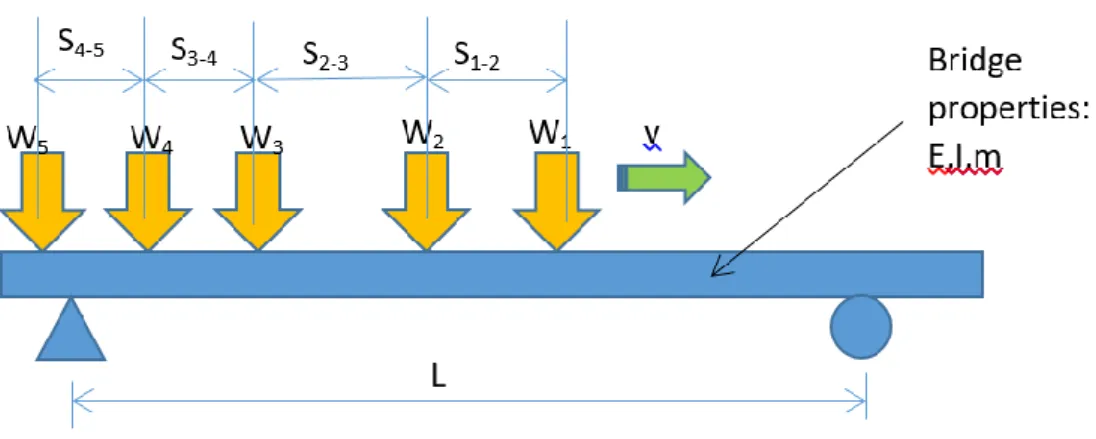
Figure 12: Simply supported beam subjected to a constant moving force
In these simulations, the bridge model is simply supported and characterized by the mass per unit length, the inertia, and modulus of elasticity, which have been assumed to remain constant
throughout the length. These properties are defined in Section 3.1.1.
The problem in Figure 12 has been solved by Frýba (1972) that defines the bending vibration of the beam, z(x,t) as:
x
x
R
t
t
x
z
t
t
x
z
x
t
x
z
EI
b
R
2 2 2 2 4 4)
,
(
2
)
,
(
)
,
(
(2) wherez(x,t) : displacement of the bridge at position x and time t,
E, and I : Young’s modulus, mass per unit length, and second moment of area of the bridge respectively,
: Dirac function, b = 2 1
1
, where is viscous damping factor (2
1
c
) and 1 is circular natural frequency of the bridge (
1
2 f
1),R : applied force,
xR = vt, is the distance of the force from the left support, where v is
velocity.
1 2 2 2 2 2 2 2 2 2 2 2 4 3cos
[cos
2
)
sin(
2
sin
4
sin
2
)
,
(
i i t i tt
e
t
i
i
t
e
i
i
i
t
i
i
i
i
i
i
L
EI
RL
t
x
z
b b
(3) whereL
v
(4) 1
v
L
(5) 21
(6) 2 2 b i i
(7)For the case of a single moving constant force, the only vehicle parameter affecting the bridge dynamic response is speed. As bridges have relatively low damping, the critical speed (speed at which the maximum deflection in forced vibration occurs) takes place when the travel time of the moving load to cross the beam span is from 0.7 to 1.0 times the fundamental period of the bridge (Michaltsos et al. 1996, Frýba 1972). Bridge deflection will decrease as vehicles increase their speed over the critical level, and bridge response will get closer to the static response as vehicles decrease their speed below the critical speed.
Strains are given by
2 2
x
z
h
g
, where hg is the distance from the strain location to the neutral axisof the section. By differentiating Equation (5) twice with respect to x, strains can be expressed as:
t
e
t
i
i
t
e
i
i
i
i
t
i
i
i
i
i
i
L
x
i
i
EI
RL
h
i t i t i g b b
cos
[cos
2
sin
2
)
(
[
sin
)
(
]
4
)
(
[
sin
8
4
2 4 2 2 2 2 2 2 2 2 2 2 2 2 2 2 2 2 1 (8)If velocity of the moving forces, v, is very small, 0 in the equation above. Then the static strain of the beam for a force at position xR = vt is given by:
2 2 1sin
sin
8
4
i
t
i
L
x
i
EI
RL
h
i g s
(9)
The dynamic component, d, can be obtained by subtracting the static strain, s, (as defined in
Equation (9)) from the total strain, (Equation (8)). This dynamic strain is provided by:
t
e
t
i
i
t
e
i
i
i
i
t
i
i
i
i
i
L
x
i
i
EI
RL
h
i t i t i g d b b
cos
[cos
2
sin
2
)
(
[
sin
]
4
)
(
[
sin
8
4
4 2 2 2 2 2 2 2 2 2 2 2 2 2 2 2 2 1(10)
Total strain at a certain point in space and time can be expressed as the sum of a static and a dynamic component ( = s + d). Hence, replacing Equation (10) into Equation (8) gives:
t
e
t
i
i
t
e
i
i
i
i
t
i
i
i
i
i
L
x
i
i
EI
RL
h
i t i t i g s b b
cos
[cos
2
sin
2
)
(
[
sin
]
4
)
(
[
sin
8
4
2 4 2 2 2 2 2 2 2 2 2 2 2 2 2 2 2 1 (11)From beam theory, the static strain for a section at location x due to a load R located at xR can be
obtained from the following two Equations:
x
L
x
L
R
EI
h
R g xR)
(
0
; 0 x xR (12))
(
L
x
L
Rx
EI
h
g R L xR
; xR x L (13)By replacing Equations (12) and (13) into Equation (11), the theoretical solution can be determined accurately with a smaller number m of mode shapes than the infinite number of Equation (8):
t
e
t
i
i
t
e
i
i
i
i
t
i
i
i
i
i
L
x
i
i
EI
RL
h
x
L
x
L
R
EI
h
i t i t m i g R g x b b R
cos
[cos
2
sin
2
)
(
[
sin
]
4
)
(
[
sin
8
4
)
(
2 4 2 2 2 2 2 2 2 2 2 2 2 2 2 2 2 1 0 0 x xR (14)
t
e
t
i
i
t
e
i
i
i
i
t
i
i
i
i
i
L
x
i
i
EI
RL
h
x
L
L
Rx
EI
h
i t i t m i g R g L x b b R
cos
[cos
2
sin
2
)
(
[
sin
]
4
)
(
[
sin
8
4
)
(
2 4 2 2 2 2 2 2 2 2 2 2 2 2 2 2 2 1 XR x L (15)In the case of a system of n concentrated moving forces, R1,R2,...,Rn, spaced at a1,a2,..an-1, from the
position of the first force with all forces travelling at speed v, the bending vibration (z(x,t)) of the beam at position x and time t will be given by:
n i i i i dx
x
R
t
t
x
z
t
t
x
z
x
t
x
z
EI
1 2 2 2 2 4 4)
,
(
2
)
,
(
)
,
(
(16) where : Dirac function,n : total number of forces,
i = 1 when force i is on the bridge (otherwise zero),
Ri : value of constant force i,
xi = vt – ai , is the position of force i (the position of first force on the
jn j i t i t j i j j j g t e t i i t e i i i i v a t i i i i i i L x i i EI L R x x h b b 1 4 2 2 2 2 2 2 2 2 2 2 2 2 2 2 2 2 2 1 cos [cos 2 sin 2 ) ( [ ) ( sin ) ( ] 4 ) ( [ sin 8 4
(17)The principle of linear superposition applies when a system of constant forces moving on a bridge at uniform speed is considered. These simple vehicle models consisting of multiple constant forces (representing the static weight) allow assessment of the impact of the static configuration of the truck (i.e., axle spacings and axle weights) in addition to speed. It is acknowledged that interaction is neglected in these preliminary calculations and that response may not be that accurate. However, previous research (González et al, 2010) has shown that these simple models can be used to estimate the underlying patterns of dynamic amplification of the bridge response in the presence of a good road profile. The magnitude of the pattern will differ from responses in more complex vehicle-bridge interaction models, but the shape will allow identifying those combinations of axle spacings and weights that are more beneficial/detrimental to the bridge response when combined with the inertial forces of the bridge. It is also possible to obtain a number of conclusions that can be generalised to multiple bridge spans and vehicle configurations. These models can establish which bridge types are vulnerable to the new configurations and what actions can be taken to ameliorate the effects.
4.2.2 Complex method using a 3D vehicle-bridge interaction model.
In a second stage, a full vehicle-bridge dynamic interaction is implemented taking into account vehicle properties such as tire and suspension stiffness and damping, and moments of inertia of the vehicle masses (Figure 13). These complex VBI simulation models are employed to investigate and quantify frequency matching phenomenon that may result from new truck configurations. The dynamic parameters of the truck models are provided in Section 2.3. A thorough review of how to implement the dynamic interaction between a sprung vehicle and a bridge can be found in Gonzalez (2010) and it is summarised here.
Figure 13. Simulation of full vehicle-bridge interaction
The response of the bridge in Figure 13 is governed by the equation:
b b b b b b b
[M ]{w } +[C ]{w } +[K ]{w } = {f } (18)
where [Mb], [Cb] and [Kb] are global mass, damping and stiffness matrices of the model respectively, b
{w },{w }b and{w }b are the global vectors of nodal bridge displacements and rotations, their velocities and accelerations respectively, and {fb} is the global vector of interaction forces between the vehicle and the bridge acting on each bridge node at time t. The size and values of [Mb], [Cb] and [Kb] depend on the type of elements employed in modelling the bridge deck. The coefficients of these matrixes are established using the Finite Element (FE) method by: (a) applying the principal of virtual displacements to derive the elementary mass, damping and stiffness matrixes and then, assembling
them into the global matrixes of the model, or (b) simply constructing the model based on the built-in code of a FE package such as ANSYS (Deng & Cai, 2010), LS-DYNA (Kwasniewski et al., 2006), NASTRAN (Baumgärtner, 1999; González et al., 2008a), or STAAD (Kirkegaard et al., 1997).
Damping is typically assumed to be viscous, i.e., proportional to the nodal velocities. Rayleigh damping is commonly used to model viscous damping and it is given by:
b b b
[C ] = α[M ] + β[K ] (19)
where and are constants of proportionality. If is assumed to be constant, and can be obtained by using the relationships = 212/(1+2) and = 2/(1+2) where 1 and 2 are the first two natural frequencies of the bridge, although can also be varied for each mode of vibration. While the equations of motion of the bridge are obtained using the FE method, there are three alternative methods to derive the equations of motion of the vehicle: (a) imposing equilibrium of all forces and moments acting on the vehicle and expressing them in terms of their degrees of freedom (Hwang & Nowak, 1991;
Kirkegaard et al., 1997
; Tan el al., 1998; Cantero et al., 2010), (b) using the principle of virtual work (Fafard et al., 1997) or a Lagrange formulation (Henchi et al., 1998), and (c) applying the code of an available FE package. The equations of equilibrium deal with vectors (forces) and they can be applied to relatively simple vehicle models, while an energy approach has the advantage of dealing with scalar amounts (i.e., contribution to virtual work) that can be added algebraically and are more suitable for deriving the equations of complex vehicle models. Similarly to the bridge, the equations of motion of a vehicle can be expressed in matrix form as:v v v v v v v
[M ]{w } +[C ]{w } +[K ]{w } = {f } (20)
where [Mv], [Cv] and [Kv] are global mass, damping and stiffness matrices of the vehicle respectively, v
{w }, {w }v and {w }v are the vectors of global coordinates, their velocities and accelerations respectively, and {fv} is the vector of forces acting on the vehicle at time t.
When analysing the VBI problem, two sets of differential equations of motion can be established: one set defining the DOFs of the bridge (Equation (18)) and another set for the DOFs of the vehicle (Equation (20)). It is necessary to solve both subsystems while ensuring compatibility at the contact points (i.e., displacements of the bridge and the vehicle being the same at the contact point of the wheel with the roadway). The algorithms to carry out this calculation can be classified in two main groups: (a) those based on an uncoupled iterative procedure where equations of motion of bridge and vehicle are solved separately and equilibrium between both subsystems and geometric compatibility conditions are found through an iterative process (
Veletsos & Huang, 1970
; Green et al., 1995; Hwang & Nowak, 1991; Huang et al., 1992; Chatterjee et al., 1994b; Wang et al., 1996;Yang &
Fonder, 1996
;Green & Cebon, 1997
; Zhu & Law, 2002; Cantero et al., 2009), and (b) those based on the solution of the coupled system, i.e., there is a unique matrix for the system that is updated at each point in time (Olsson, 1985; Yang & Lin, 1995; Yang & Yau 1997;Henchi et al., 1998
; Yang et al., 1999, 2004a;Kim et al., 2005
; Cai et al., 2007; Deng & Cai, 2010; Moghimi & Ronagh, 2008a). The use of Lagrange multipliers can also be found in the solution of VBI problems (Cifuentes, 1989; Baumgärtner, 1999; González et al., 2008a).A step-by-step integration method must be adopted to solve the uncoupled or coupled differential equations of motion of the system. These numerical methods break the time down into a number of steps, Δt, and calculate the solution w(t+Δt) from w(t) based on assumed approximations for the derivatives that appear in the differential equations. They are different from methods for single-DOF systems because most FE models with lots of DOFs poorly idealise the response of the higher modes, and the integration method should have optimal dissipation properties for the removal of those non-reliable high frequency contributions. Fourth-order Runge-Kutta is a popular integration method in the solution of large multi-DOF VBI systems (Frýba 1972; Huang et al., 1992; Wang & Huang, 1992; Cantero et al., 2009; Deng & Cai, 2010). Acceleration is expressed as a function of the other lower derivatives and a change of variable transforms the second order equation into two first order equations. Then, the recurrence formulae of fourth-order Runge-Kutta is employed to approximate
4.3.1 The bridge model
4.3.1.1 Typical properties of bridges up to 21 m
Typical properties for short and medium-span bridges are given here for reference purposes. Bridge parameters depend on the cross section of the bridge which is related to the span length. Given that the range of interest is between 10 m and 20 m, the most common sections for these spans are inverted concrete T-beam bridge models, which are used to extract typical mechanical properties. All bridge models here are assumed to be of concrete construction with a Young’s Modulus of 3.5x10¹⁰ N/m2 and a density of 2500 kg/m3. The inverted T-beam section is illustrated in Figure 14.
Figure 14. Cross-section of Inverted T-beam bridge model.
A ratio span to depth is 1/20 and a width of 15 m are employed. Based on these values, mass per unit length (μ) and second moment of area (J, assumed constant across the bridge length L) are as follows:
2500 15
20
L
u
(21)
315
20
12
L
J
(22)Table 6 gives the values of mass per unit length, inertia and main natural frequency for an inverted-T beam bridge model, as a function of span length.
Table 6: Typical parameters for inverted-T beam bridges (Li 2006)
Span Length (m) E (N/m2) Density (kg/m3) μ (kg/m) J (m4) Frequency (Hz) 9 3.50E+10 2500 16875 0.113906 9.42 11 3.50E+10 2500 20625 0.207969 7.71 13 3.50E+10 2500 24375 0.343281 6.52 15 3.50E+10 2500 28125 0.527344 5.65 17 3.50E+10 2500 31875 0.767656 4.99 19 3.50E+10 2500 35625 1.071719 4.46 21 3.50E+10 2500 39375 1.447031 4.04
If width, depth, density or modulus of elasticity of the specific bridge to be assessed varied with respect to those values assumed in this section, the expected properties provided in Table 6 would need to be corrected accordingly.
Other forms of construction, such as steel beams and RC deck slab, can also be found in the European bridge stock. Those forms are, however, not considered here. Beam-and-slab deck constructions have
a poorer load transfer than slab deck sections, i.e., a significant percentage of the load is taken by the beams directly underneath the points of application of the load.
4.3.1.2 Bridge model
In Section 4.2.1 (simple assessment), the bridge is modeled as a simply supported beam and three bridge spans with properties provided in Erreur ! Source du renvoi introuvable. are investigated. Damping ratio is assumed to be 0.03 in all cases.
Table 7: Bridges under investigation in Section on “Simple assessment”
In Section 4.2.2 (detailed assessment), a simply supported solid slab plate deck model is used to represent a 15 m long bridge. This structural type and span is commonly found in short-span bridges (i.e., one which permits a 2-lane carriageway beneath). It also allows a single vehicle event made of a 5-axle truck to fully fit within the bridge length. The bridge is modeled as an orthotropic thin slab. It consists of rectangular C1 plate elements having four nodes. There are four DOFs at each node of the
C1 plate element: one vertical displacement, one twist and two rotations (in X and Y direction);
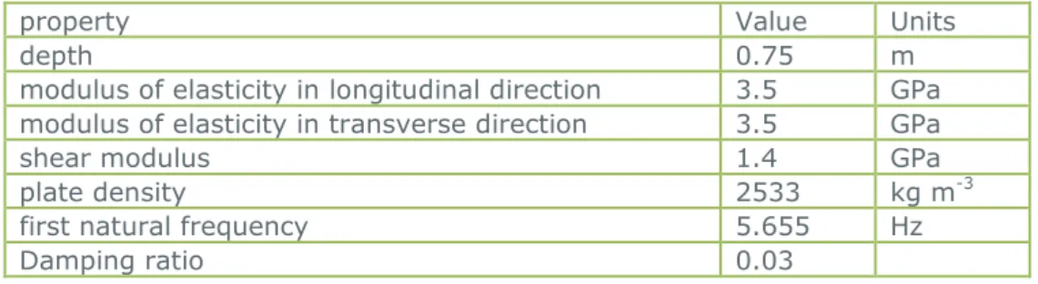
therefore, there are 16 DOFs in the element. When compared to the normal Kirchhoff’s plate element, there is one extra DOF per node in this element to avoid the discontinuity of slope across the edge elements. An area of 15 m (length) x 11 m (width) is encompassed by the slab FE model, which is then discretized into 0.5 m x 0.5 m C1 plate elements. Erreur ! Source du renvoi introuvable. gives the properties for the plate bridge model.
Table 8: Properties of plate model employed in Section on “Detailed assessment”
property Value Units
depth 0.75 m
modulus of elasticity in longitudinal direction 3.5 GPa modulus of elasticity in transverse direction 3.5 GPa
shear modulus 1.4 GPa
plate density 2533 kg m-3
first natural frequency 5.655 Hz
Damping ratio 0.03
4.3.2 The road profile
4.3.2.1 Generation of the road profile
The detailed assessment of Section 5 incorporates a road carpet (profile of the pavement) in addition to the deck construction. A road profile r(x) can be theoretically generated from power spectral density functions as a random stochastic process:
N
d k k i
i=1
r(x)=
2G (n )Δncos(2πn x-θ )
(23)where Gd(nk) is power spectral density function in m2/cycle/m; nk is the wave number (cycle/m); i is a random number uniformly distributed from 0 to 2;Δnis the frequency interval (Δn = (nmax–nmin)/N where nmax and nmin are the upper and lower cut-off frequencies respectively); N is the total number of waves used to construct the road surface and x is the longitudinal location for which the road height is being sought. The road class is based on the roughness coefficient a (m3/cycle), which is related to the amplitude of the road irregularities, and determines Gd(nk). Gd(nk) is equal to a/(2nk)2. ISO standards specify ‘A’, ‘B’, ‘C’, ‘D’ and other poorer road classes depending on the range of values where a is located (
ISO 8608, 1995
). For a given roughness coefficient, different road profiles can be obtained varying the random phase angles i. The height of the road irregularities are correlated inLength(m) L
Mass per unit length m (kg/m) Second moment of inertia J (m4) 1st natural frequency f1 (Hz) 10 18750 0.1609 8.609 15 28125 0.5273 5.655 20 37500 1.25 4.24
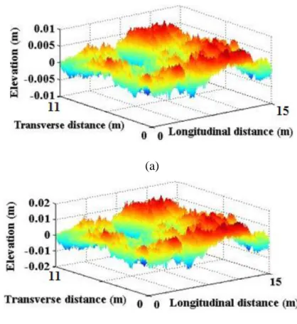
In Section 4.5, two types of road classes according to ISO 8608 are considered: Class ‘A’ (i.e., ‘very good’ with Gd(n0) = m3/cycle) and Class ‘B’ (i.e., ‘good, with Gd(n0) = m3/cycle), which are to be expected in well maintained highways. A moving average filter is applied to the generated road profile heights over a distance of 0.24 m to simulate the attenuation of short wavelength disturbances by the tyre contact patch. Figure 15 illustrates two road carpets of classes ‘A’ and ‘B’ generated for the bridge surface. In addition to the bridge carpets, an approach length of 100 m road has been added to initially excite the vehicle before moving onto the bridge.
(a)
(b)
Figure 15. Two samples of road carpets generated for the bridge: (a) Class ‘A’ and (b) Class ‘B’
4.4 Simple assessment
In a first simple assessment, models of moving constant forces (Section 4.2.1) crossing planar bridge models are used to calculate DAmF. Critical speeds causing a largest DAmF are identified for three truck configurations (Table 1). Following the work plan devised in the methodology report, these first results correspond to a relatively simple model of series of forces traversing three bridges with different span lengths (Table 7). The focus is on small spans as long spans will be governed by a traffic jam where dynamic effects are not of that relevance. However, 5-axle trucks can become part of a critical load scenario in short span bridges. In these first results, planar beam models are employed and the interaction between vehicle and bridge is neglected. The simulation model is illustrated below.
Figure 16: Simple planar simulation model
The simulation model employed here implies that the static value of the truck axles and inertial forces of the bridge are taken into account, but the effect of road profile and vehicle dynamic properties are ignored. The purpose of this relatively simplistic model is to analyse the impact of static mechanical properties of the truck (i.e., axle spacings and axle weights) on the response in isolation from the vehicle dynamic parameters. The models are planar, i.e., series of concentrated loads running on a simply supported bridge beam model. More complex simulations taking into account vehicle dynamic properties will take place further on, allowing to assess the percentage dynamic amplification of a bridge due to different parameters (static and/or dynamic) of the truck.
The solution of the bending moment response of any section of the beam model to the moving loads is governed by truck parameters (static axle weights W1, W2, W3, W4 and W5 and axle spacings S1-2, S2-3, S3-4, S4-5 and vehicle velocity v) and bridge parameters (section location, bridge length L, and properties of mass per unit length m, modulus of elasticity E and inertia I). Details on the resolution of this problem have been provided in Section 4.2.1. The parameters of the three bridge spans are defined in Table 7 and the three truck configurations are given in Table 1. By combining all, it is possible to obtain results for 9 different scenarios. In the simulations, the beam is discretized into elements 0.1 m long and time step for calculations is 0.002 seconds.
4.4.1 Definition of parameters
The bending moment in the bridge structure is time-varying as the truck moves across the bridge. Following Equation (1), DAmF is defined here as:
DAmF = Maximum total bending moment at section holding maximum static response / Maximum static bending moment at section holding maximum static response
The definition of Full Dynamic Amplification Factor (FDAmF) is defined as follows:
FDAmF = Maximum total bending moment anywhere on the bridge / Maximum static bending moment at section holding maximum static response
Clearly, FDAmF is always greater than or equal to DAmF.
In the graphs that follow, the term alpha is employed. Alpha is a non-dimensional term that relates vehicle speed to the first natural frequency of the bridge as follows:
Alpha = (Vehicle speed/Bridge Length) / (2*First Natural Frequency of bridge in Hz)
Figure 17 provides a quick reference to obtain actual numbers and units that correspond to normalized and dimensionless values in the text. For example, a vehicle speed of 120 km/h (=33.33 m/s) results into alpha values of 0.194, 0.197 and 0.196 for the 10, 15 and 20 m bridge spans respectively.
(a) (b)
Figure 17. Simulation parameters involving load speed: (a) Load frequency (Hz), (b)
Normalized speed parameter .
4.4.2 Results of simple assessment
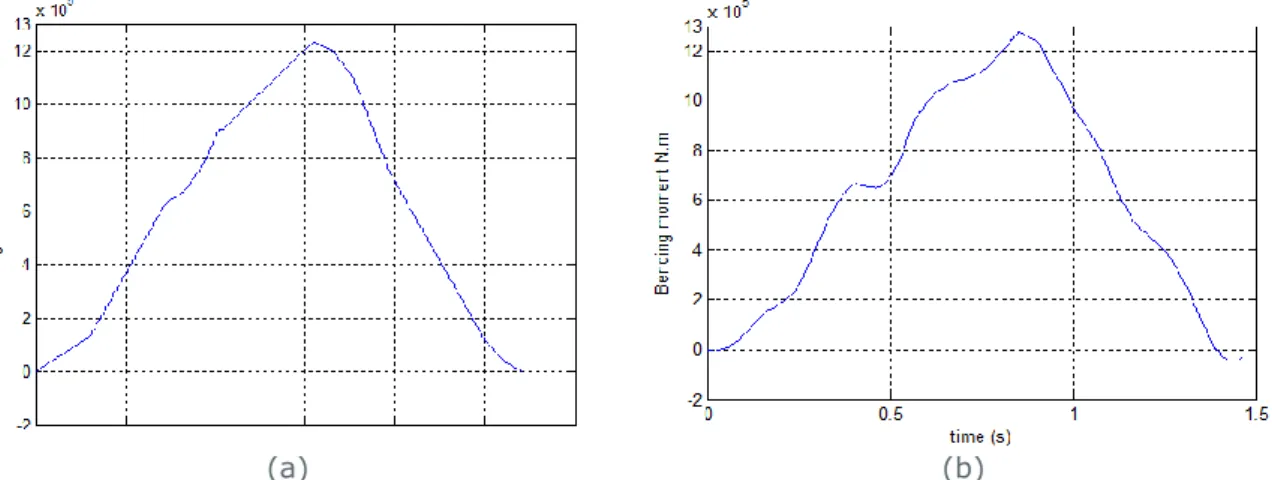
The results in this section are obtained from processing the information from static and total bending moments at every section of a bridge for a wide range of truck speeds. From the section holding the maximum static response, it is possible to obtain DAmF for each speed (and as a result, DAmF-speed patterns). Taking into account every possible bridge cross-section (longitudinal abscissa) (not only the one holding the maximum static response), it is then possible to obtain FDAmF. For example, the two figures below illustrate two bending responses (static and total at 80 km/h) due to truck type C at a section 8.7 m from the left support (where static effect is maximum) on the 20 m bridge.
(a) (b)
Figure 18. Bending moment-time history: (a) Static bending moment at mid-span of 20 simply supported beam due to truck type C; (b) Total bending moment at midspan of 20 simply supported beam subjected to truck type C travelling at 80 km/h
4.4.3 Results for Truck Type A
The next table indicates the maximum static bending moment and the location in the bridge with respect to the first support where it occurs.
Table 9: Maximum static moment and its bridge location for truck A
Bridge length(m)
L Max. static effect value kN.m Location of maximum static load effect from the left support (m)
10 454.27 5.1
15 757.53 6.3
20 1191.6 8.7
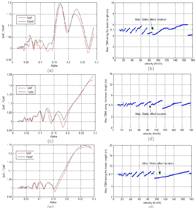
In the left-hand figures that follow, it is possible to see how DAmF and FDAmF varies with alpha (or normalized vehicle speed) for each bridge span. The existence of critical speeds that will excite the bridge to a larger extent is evident. In the right-side figures, it is possible to see where the maximum total moment (static + dynamic) occurs for each speed and for each span under investigation. It is worth noticing that the maximum bending moment does not necessarily occurs at midspan or even
0 20 40 60 80 100 120 140 160 180 200 Load speed (m/s) 0 0.1 0.2 0.3 0.4 0.5 0.6 0.7 0.8 0.9 0 10 20 30 40 B rid g e le n g th ( m ) L f=0.5 Lf=1 Lf=1.5 L f=2 L f=2.5 0 2 4 6 8 10 12 14 16 18 20 0 10 20 30 Load frequency (Hz) 1 s t Na tu ra l f re q u e n cy (Hz) =0.1 =0.2 =0.3 =0.4 =0.5
where the maximum static load effect occurs, due to the added dynamic effect. Unlike the static effect, the dynamic effect and the location of the dynamic peaks vary with speed.
(a) (b)
(c) (d)
(e) (f)
Figure 19: Results for truck ‘A’: (a) FDAF and DAF versus Alpha of 10 simply supported beam subjected to truck type A; (b) Location of max. total BM throughout the 10 m beam length versus velocity of truck type A; (c) FDAF and DAF versus Alpha of 15 simply
supported beam subjected to truck type A; (d) Location of max. total BM throughout the 15 m beam length versus velocity of truck type A; (e) FDAF and DAF versus Alpha of 20 simply supported beam subjected to truck type A; (f) Location of max. total BM throughout the 20 m beam length versus velocity of truck type A.
4.4.4 Results for Truck Type B
Similarly to results above, Table 10 indicates the maximum static bending moment due to Truck B and the location in the bridge with respect to the first support where it occurs. As expected (the three truck configurations being tested are similar), differences with respect to truck A are very small, although a consistent larger maximum static effect value can be noticed for the three bridge spans under investigation.
Bridge Length(m)
L Max. static effect value kN.m Location of maximum static effect from the left support (m)
10 469.56 5
15 785.47 6.9
20 1235.5 8.8
For comparison purposes, the same DAmF and FDAmF graphs versus speed and critical location holding the maximum total moment are generated for the truck B below.
(a) (b)
(c) (d)