Thermodynamic Modelling Of A Pistons Engine: Calculation Of The Nox Emissions

Texte intégral

(1)Journal of Fundamental and Applied Sciences ISSN 1112-9867 Available online at. http://www.jfas.info. THERMODYNAMIC MODELLING OF A PISTONS ENGINE: CALCULATION OF THE NOX EMISSIONS N. Mahfoudi * and M. Kadja. University of Constantine, laboratory of energetic applied and pollution, 25000, Algeria. Received: 27 December 2012 / Accepted: 27 June 2013 / Published online: 30 June 2013. ABSTRACT The internal combustion engines are under development remarkable these last decades, but they represent, currently, a very important source of polluting gas emissions. The nitrogen oxides (NOx) form part of these polluting emissions, and have a harmful effect on human health, as well as the environment. Considering the complexity of the process of formation of the latter, many numerical simulations were developed, our work, allows the calculation of the nitrogen oxide rate (NO) in exhaust gases, starting from the developed equations of the chemical kinetics, while being based on the thermal mechanism of Zeldovich. Simulation is carried out for a gasoline engine, and the results obtained show that: the maximum of NO concentrations corresponds to an equivalent ratio of 0,9. For leaner or richer equivalence ratios, concentration decreased. The NO concentrations depend of various parameters (spark timing angle, combustion duration, and engine speed). Key words: Exhaust gases, spark-ignition-engine, chemical kinetics, numerical simulation.. 1. INTRODUCTION The development of our civilization without precaution lets now appear consequences of the emissions of pollutants whose cumulated volume is not negligible for our planet: destruction of drills by the acid rains, reheating of the atmosphere (effect of greenhouse), disappearance of species….. Author Correspondence, e-mail: nadjiba213@Yahoo.fr ICID: 1042340.

(2) N. Mahfoudi et al.. J Fundam Appl Sci. 2013, 5(1), 96-109. 97. The internal combustion engines represent an important source of pollution, which pushed research to be directed towards this kind of source, with an aim of reducing them. Since the principal mechanisms of formation of the various pollutants are of thermal nature, it was necessary to analyze the thermodynamic cycle of the engine. Various researches were developed in this way (S. Saravanan and Al , 2012; F.Scappin and Al, 2012; C.D. Rakopoulos and Al, 2011; Mustafa Koç and Al, 2009; S. Murillo and Al, 2005 ). In this context, this study presents a modelling of the thermodynamic cycle of a pistons engine whose objective is the calculation of the concentrations of one of the principal pollutants, constituting exhaust fumes, the nitrogen oxides known under the NOx notation.. 2. BACKGROUND The development of the simulation of the thermodynamic cycle of the internal combustion engines, refer at the beginning of the Sixties. With remarkable advanced of sciences of data processing, numerical simulation became an important means which makes possible to understand the various phenomena. The first simulations were based on the mono zone model, then the models was developed and extended to two, three and several zones. Patterson and Van Wylen (1964) were among the first which introduced the zones burnt and unburnt residues, progressive combustion, the heat transfer and propagation of flame in the study of the engines with homogeneous load. These studies took part in an important way in the advance and development of thermodynamic simulations. Heywood and Al (1979) have described the first simulations which use multiple zones for the process of combustion. For their formulation, the burnt zone was divided into adiabatic core and zone of boundary layer, in addition to the unburnt zone. Blumberg and Al (1980) used the multizones model and confirmed that the introduction of boundary layer zone, allows a better representation of the losses of heat in the vicinity of the walls. James (1982) also presented his observations on the importance of the multizones models to predict the NOx emissions. Raunie and Al (1995) published the results of cycle simulation using multiple zones. For the burnt gases, they could show the particularly importance of these zones to calculate the nitric oxides concentration. This work doesn’t include the boundary layer zone and flows..

(3) N. Mahfoudi et al.. J Fundam Appl Sci. 2013, 5(1), 96-109. 98. Other works were carried out on the same way, by considering other parameters such as flow, turbulence in the cylinder, the detailed models of the heat transfer and the propagation of the flame (Chamiak et al.., 1991, Wahiduzzman and Al, 1993). Very recent works, was completed by Caton and Al (2000, 2001, 2002, 2003) being based on the model at three zones (burnt, unburnt, and boundary layer). The results obtained by this simulation (pressure and instantaneous temperature in the cylinder) were used in the calculation of the rate of NOx emitted by the engine. Taking into account the direct influence of the operating parameters on the results of simulations, parametric studies were published by the same author. An experimental research into the use of LPG in spark-ignition outboard engines is presented by S. Murillo and Al (2005). The results obtained indicate that with the use of LPG, specific fuel consumption and CO emissions were much lower without noticeable power loss while HC emissions are shown to be little affected by fuel substitution. In contrast, NOx emissions were higher, but could be kept below current and future emission limits. In 2009 Mustafa Koç and Al studied the interest to use ethanol like fuel. The results of the engine test showed that ethanol addition to unleaded gasoline increase the engine torque, power and fuel consumption and reduce carbon monoxide (CO), nitrogen oxides (NOx) and hydrocarbon (HC) emissions. C.D. Rakopoulos and Al (2011) also studied the effect of an alternative fuel (Hydrogen) in NOx emissions. They combined experimental and numerical study. The previously studies, were carried out on a spark ignition engine. The Diesel engine is an important source of the NOx emissions, for this cause several simulations, were carried out for this type of engine. Considering the complexity of the process of combustion in a diesel engine, due to the various parameters which manage this process (heterogeneity of combustion, injector’s forms …), several empirical sub models, were proposed by various researchers (Austen and Lyn, 1960-61; Whitehorse and Way, 196970). With the necessity to the precise predict of the polluting emissions in the exhaust phase, researchers tried to develop a combustion models at two zones (Khanet et al.., 1971; Whitehouse and Sareen, 1974; Kouremenos et al., 1989).. Thereafter, some multizones. models appeared (Shahed and Al, 1975; Hodgetts and Shroff, 1975; Hiroyasu and Al, 1987; Kouremenos and Al, 1987), carrying the disadvantages of the first attempts. In this moment, the multidimensional models are very useful for better including/understanding the course of combustion. However, those are limited by l’insuffisance relative under models of turbulence and the chemistry of combustion..

(4) N. Mahfoudi et al.. J Fundam Appl Sci. 2013, 5(1), 96-109. 99. The research carried out by Rakopoulos et al. (1995), Rakopoulos and Hountalas (1998, 2000), Rakopoulos and Al. (2003), form a part of a long line of the recent multizones philosophies applied to the simulation of the Diesel engine (DI) cycle, while being based on the model at two zones, sight its simplicity, as well as the availability of details concerning the various mechanisms implied in combustion. A review of chemical characterization of particulate emissions from diesel engines done by M. Matti Maricq (2007) examined the chemical properties of particulate matter (PM) in diesel vehicle exhaust at a time when emission regulations, diesel technology development, and particle characterization techniques are all undergoing rapid change. The operation of four – stroke diesel engines in either propulsion or generator mode application has a strong influence on gaseous, smoke (soot) and particulates emissions. This effect was studied by A. Sarvi and Al (2008). Modeling NOx formation stays until the daytime a challenge. The researches of S. Saravanan and Al (2012), F.Scappin and Al (2012) show that.. 3. MODEL DESCRIPTION The engine used in this study, is the spark ignition engine. Thermodynamic modelling consists in the mathematical equations managing each phase of the four-stroke cycle including the intake, compression, combustion, expansion and exhaust processes. For this reason, the major assumptions and approximations used in the development include the following: . The thermodynamic system is the mixture contained in the cylinder.. . The mixture contained in the cylinder is homogeneous in space during all the phases of the cycle.. . For a multicylinder engine, all the cylinders are identical, having same thermodynamics and functioning under the same conditions, therefore the total results, are obtained by multiplying the results of analyse of one-cylinder by the number of cylinders.. . For the simplicity of the model, the combustion chamber has a cylindrical form.. . The mixture contained in the cylinder, occupies a zone during the processes of compression, relaxation and exhaust.. . The mixture, during the combustion phase is divided into two zones: one contains burnt gases, and the other, the unburned gases.. . The thermodynamic properties (including pressure and temperature) vary only with time (crank angle) and are spatially uniform in each zone.. . The gases are perfect gases..

(5) N. Mahfoudi et al.  . J Fundam Appl Sci. 2013, 5(1), 96-109. 100. The fuel is completely vaporized and mixed with the incoming air. The intake and exhaust manifolds are infinite plenums containing gases at constant temperature and pressure.. . At compression, the system is closed.. . The instantaneous thermodynamic properties are obtained from JANAF tables [1] based on the appropriate compositions.. The modelling of each phase of the cycle makes it possible to obtain the equations which controls it. The pressure at the end of intake process is a principal factor which conditions the mass gas introduced during the intake phase. Its value is determined by the following formula:. Pa  P0  Pa. (1). “∆Pa” Loss of pressure generated by the geometrical, aerodynamic parameters and acoustics of the intake system. Its value is calculated according to the equation of Bernoulli applied for gases in permanent flow. The temperature at the end of the intake depends on the characteristics of the high-carbon mixture, at the beginning of intake, and of residual gases. It is given by the following formula [2]:. Ta . T0  T   r .Tr 1  r. (2). The coefficient of residual gases is given by the following expression [2]:. r . T 0.  T  Pr . T0  . Pa  Pr. (3). A one-zone formulation is appropriate for the compression and process, the first law of thermodynamics. During these phases, it is necessary to determine the variations of volume, the pressure and the temperature of the mixture, as function of the time (crank angle). For the one-zone formulation for this system is:. dm dE dQ dW dmin    .hin  out .hout d d d d d. (5). The application of the equation (5) makes it possible to obtain a system of differential equations, which determine the instantaneous temperature, pressure and volume during the compression phase. For the combustion process, two zones are used: unburned and burned zone, between which it has mass transfer (figure1)..

(6) N. Mahfoudi et al.. J Fundam Appl Sci. 2013, 5(1), 96-109. Intake. 101. Exhaust. Fig.1. Schematic of Thermodynamic system during combustion. The energy equations for the two zones are:. d ( m.u ) b dQ b dV dm b   P. b  .hu d d d d. (6). d ( m .u ) u dQ u dV dm u   P. u  .h u d d d d. (7). Derivatives for the two temperatures, the pressure, and the two volumes may be derived.. 4. ITEMS FOR THE GAS TEMPERATURE DERIVATIVE EQUATION To solve the above governing differential equations (eq. 5, 6 and 7), several items are needed. These items include the thermodynamic properties, the mass fraction burned, the convective heat transfer, and the mass flow rates. These items are described next.. 5. MASS FRACTION BURNED: The mass fraction burn can be determined by the relation of Wiebe [3]-[5]-[6], given by the formula:. x  1  exp[  a .Y m 1 ] Where y is a non-dimensional time variable. (8).

(7) N. Mahfoudi et al.. Y. J Fundam Appl Sci. 2013, 5(1), 96-109. 102.  s b. “a” and “m” are parameters that are selected to provide a match with experimental information. The values that provide a good match with the data depend on complex functions of the turbulence, chemistry, fuel, equivalence ratio, chamber geometry, and a number of other features. The values used here are based on the work of Heywood et al. Heywood [7]. a=5.0 and m=2.2. 6. HEAT TRANSFER The overall heat transfer to the cylinder gases is given by:. dQ  hc .S ( ).(Twall  T ) dt. (9). During the combustion process, the total heat transfer is allocated to the various zones (but the total is still given by eq. 6). For this work, the quantity of heat transmitted by unburned gases is given by the following relation [8]:. dQu  Vu     d  Vtot . 2/3.  T  Tu . wall T T avg  wall.  dQtot .  d . (10). The quantity of heat transmitted by burned gases is calculated according to the formula: dQb dQu dQtot   d d d. (11). 7. KINETICS OF FORMATION OF NO To simulate the formation of NO, starting from the equations of the chemical kinetics, the Zeldovich model was used, described by following chemical reactions: K1 O  N 2  NO  N. (1). K2 N  O 2  NO  O. (2). K3 N  OH  NO  H. (3). This mechanism makes it possible to calculate the concentration of NO according to the following formulas:. 2 . R 1 .( 1   2 ) d [ NO ]  dt (1   . K ). (12).

(8) N. Mahfoudi et al.. J Fundam Appl Sci. 2013, 5(1), 96-109. 103. With:. R1  K 1d .[O ]e .[ N 2 ]e  K 1i .[ NO ]e .[ N ]e R2  K 2 d .[ N ]e .[O2 ]e  K 2 i .[ NO ]e .[O ]e R3  K 3d .[ N ]e .[OH ]e  K 3i .[ NO]e .[ H ]e K. . [ NO ] [ NO ]e. R1 R2  R3. “[X]e” is the equilibrium concentration of species X. The resolution of the equation (12), determine the instantaneous nitric oxide concentration. For the resolution of the various systems of differential equations, the method of Runge Kutta was selected and showed a satisfying time of convergence.. 8. RESULTS AND DISCUSSION The characteristics of the engine used for this simulation, according to the conditions used by Caton [8], as well as other parameters considered, are summarized in the table following: Table 1. Engine Specifications for Computations. Item. Value. Number of cylinders. 1. Bore (mm). 101,6. Stroke (mm). 88,4. Crank Rad/Con Rod. 0,305. Spark Timing (°bTDC). 40. Combustion duration. 80. Speed of engine (rpm). 3000. Fuel. Isoctane. Figures 2 and 3, show cylinder pressure and the temperature of burnet gases as function of crank angle during the combustion and expansion phase, for an equivalent ratio of 0.9. The compression phase is initiated at 180° BTDC until 30° BTDC, angle who correspond to the spark timings. The cylinder average pressure increases from 0,1 MPa (Pressure at end of the intake) to a value of end of compression defined according to compression ratio's. Combustion begins at 30° BTDC and is completed at 30° ATDC, which corresponds to a duration of 60° during which the pressure continues to increase to a maximum value (~3,4.

(9) N. Mahfoudi et al.. J Fundam Appl Sci. 2013, 5(1), 96-109. 104. MPa) in the vicinity of the TDC, then decrease and continuous to decrease until the end of the expansion phase. The burnet gases temperature increases gradually with the advance of combustion to reach its maximum value (~2750 K) in the neighbourhoods of the TDC, then decreases until the end of. 3.5. Combustion Phi= 0.9 Tetas= - 40° BTDC Tetab= 80° Rrot= 3000 rpm. 3.0. 2.5. PRESSURE (MPa). BURNET GASES TEMPERATURE (°K). the expansion, to reach minimal values.. 2.0. 1.5. 1.0. 0.5. -1.0. -0.5. 0.0. 0.5. 1.0. 1.5. 2.0. 2.5. 3.0. 2800. Combustion. 2400. 2200. 2000. 1800. 1600 -1.0. 3.5. Phi= 0.9 Tetas= - 40° BTDC Tetab= 80° Rrot= 3000 rpm. 2600. -0.5. 0.0. 1.5. 2.0. 2.5. 3.0. 3.5. Combustion. Phi= 0.9 Tetas= 40°BTDC Tetab= 80° Rrot= 3000 rpm. 1400. NO (ppm). 1.0. Fig.3. Burned gases temperature as function of crank angle during the combustion and expansion phase. Fig.2. Cylinder pressure as function of crank angle during the combustion and expansion phase. 1600. 0.5. CRANK ANGLE. CRANK ANGLE. 1200. 1000. 800. 600 -0.5. 0.0. 0.5. 1.0. 1.5. 2.0. 2.5. 3.0. 3.5. CRANK ANGLE. Fig.4. NO concentration as function of crank angle during combustion and expansion phase. To calculate the instantaneous concentration of NO, the Zeldovich model is used. For the conditions presented on figure 4 the nitric oxide begins to form significantly after about 10°V ATDC..

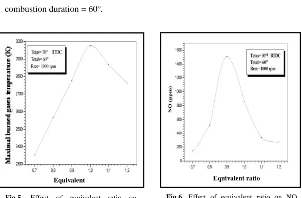
(10) N. Mahfoudi et al.. J Fundam Appl Sci. 2013, 5(1), 96-109. 105. With the increase of temperature, the NO concentration increases to reach a maximum value (~ 1500 ppm, [9]), then is stabilized on this level, because of the freezing of the dissociation reactions due to the short residence time. To validate the computer code, a parametric study was used taking account the various operating parameters of the engine (equivalent ratio, spark timing, combustion duration, engine speed…) for the following operating conditions:  Spark timing = 30° BTDC ; . Engine speed = 1000 rpm ;. . combustion duration = 60°.. Equivalent ratio. Equivalent ratio. Fig.5. Effect of equivalent ratio maximal burned gases temperature. on. Fig.6. Effect of equivalent ratio on NO concentration. The maximum of burned gases temperature increases with the equivalent ratio to reach a maximum at 1, then decreases for the equivalent ratio higher than 1(figure 5). The NO concentration has also the same variation as the temperature, to only one difference, the maximum corresponds to an equivalent ratio equal to 0,9(figure 6). Figure 7 illustrates the variation of the NO concentration as function of the equivalent ratio for various values of spark timing. The maximum of the nitrogen oxide concentration increases with the angle of spark timing, and always corresponds to an equivalent ratio equal to 0.9. The comparison of the results schematized on figure 7, with those measured by Nebel and Jackson (1958) and the results of a simulation carried out by Caton and al. [9], indicates an acceptable agreement concerning the shape of the curves as well as the maximum values.

(11) N. Mahfoudi et al.. J Fundam Appl Sci. 2013, 5(1), 96-109. 106. which according to the experiment, are included between 800 and 4300 ppm, for the conditions of this simulation [9, 11]. As certain details of calculation are unknown at the beginning (some parameters of the engine, combustion duration …), this level of agreement is acceptable.. Equivalent ratio. Fig.7. Effect of spark timing NO concentration 9. CONCLUSION According to the results, the following conclusions can be drawn: . For the measured or calculated values, the maximum of NO concentrations corresponds to an equivalent ratio equal to 0,9. For leaner or richer equivalence ratios, the nitric oxide concentration decreased.. . The NO concentrations increase with spark timing angle.. . The computed nitric oxide computations dependent on the values of the combustion duration.. . The NO concentration decreases by increasing the engine speed.. In general, the procedures of calculation used in this work, include the principal factors influencing the formation of nitrogen oxide.. 10. NOMENCLATURE ATDC: After Top Dead Center BTDC: Before Top Dead Center dE/dθ: Internal energy variation of the system. ..

(12) N. Mahfoudi et al.. J Fundam Appl Sci. 2013, 5(1), 96-109. dP/dθ: Variation of system pressure. dQ/dθ: Heat flow exchanged with the walls. dW/dθ: Work variation of the système. h: Spcifique Enthalpy of gases. hc: Convective heat transfer coefficient h.dm/dθ: Flow enthalpic Ki:Kinetics constante of reaction m : Mass of gases P: Pressure of gase. S(θ) : Wall area. T : Gases température. Tavg : Avreage cylinder gas temperature. Twall: Walls température Vuni: Cylinder volume. x: Mass fraction burned. [X]: Volumetric concentration of species X Y: fraction of burn duration [X]e: Equilibrium concentration of species X Greek and other symbols: ∆Pa: Loss of pressure of the intake system. ∆T: Rise in the temperature γr: Coefficient of residual gases ε : Volumetric rate of compression θ : Instantaneous crank angle θb : Combustion duration θs : Crak angle of start of combustion. Indiccations and exhibitors: 0 : Index indicating the parameters of the beginning of admission. a: Index indicating the parameters of the end of admission. b :Burned. r : Index indicating the parameters of residual gases. u : Unburned.. 107.

(13) N. Mahfoudi et al.. J Fundam Appl Sci. 2013, 5(1), 96-109. 108. 11. REFERENCES [1] Chase et al., JANAF Thermochemical Tables, J. Phis. chem, Ref. Data, Vol.14, No.1, 1987. [2] A. Makartchouk, Diesel Engine Engineering, thermodynamics, Dynamics, Design and control, Ed. Marcel Dekker, 2002, pp.1-4, 19-59. [3] J. A. Caton, Detailed result for nitric oxide emissions as determined from multi-zone cycle simulation for a spark-ignition engine, Fall Technical conference of ASME-ICED, New Orleans, 08-11 Septembre 2002. [4] J. A. Caton, Effects of the compression ration on nitric oxide emissions for spark-ignition engine: Results from a thermodynamic cycle simulation, Int. J. Engine Res, Vol. 4, No. 4, March 2003, pp. 249-268. [5] P. Arqués, Inflammation combustion- pollution, Ed. Masson, Paris, 1992, pp.109-123. [6] P. Arquès, La combustion, Inflammation-combustion-Pollution. Application, Ed. Ellipses, Paris, 2004, pp. 67-128, 143-173. [7] J.C.Guibert, Carburants et moteurs, Technologie - Energie – Environnement, Tome 2, Ed.Technip, Paris, 1997, pp. 470-488, 490-507. [8] J.. A.. Caton,. A. multiple-zone. cycle. simulation. for. spark-ignition. engines:. Thermodynamics details, 2001 Fall Technical conference of ASME-ICED, Argonne, 23-26 septembre 2001. [9] J. A. Caton, The use of three-zone combustion model to determine nitric oxide amissions from a homogeneous-charge, spark-ignited engine, spring technical conference of ASMEICE, Salzburg, Australie, 11-14 Mai, 2003. [10] S. Murillo, J.L. Míguez, J. Porteiro, L.M. López González, E. Granada, J.C. Morán, LPG: Pollutant emission and performance enhancement for spark-ignition four strokes outboard engines, Applied Thermal Engineering, 2005, 25 (13), 1882–1893. [11] Mustafa Koç, Yakup Sekmen, Tolga Topgül, Hüseyin Serdar Yücesu, The effects of ethanol–unleaded gasoline blends on engine performance and exhaust emissions in a sparkignition engine, Renewable Energy, 2009, 34 (10), 2101–2106. [12] C.D. Rakopoulos, G.M. Kosmadakis, J. Demuynck, M. De Paepe, S. Verhelst, A combined experimental and numerical study of thermal processes, performance and nitric.

(14) N. Mahfoudi et al.. J Fundam Appl Sci. 2013, 5(1), 96-109. 109. oxide emissions in a hydrogen-fueled spark-ignition engine, International Journal of Hydrogen Energy, 2011, 36 (8), 5163–5180. [13] M. Matti Maricq, Chemical characterization of particulate emissions from diesel engines: A review, Journal of Aerosol Science, 2007, 38(11), 1079–1118. [14] Arto Sarvi, Carl-Johan Fogelholm, Ron Zevenhoven, Emissions from large-scale medium-speed diesel engines: 1. Influence of engine operation mode and turbocharger Fuel Processing Technology, 2008, 89 (5), 510–519. [15] S. Saravanan,. G. Nagarajan,S. Anand,. S. Sampath, Correlation for thermal NOx. formation in compression ignition (CI) engine fuelled with diesel and biodiesel, Energy, 2012, 42 (1), 401–410. [16] F. Scappin, S. H. Stefansson, F. Haglind, A. Andreasen, U.Larsen, Validation of a zerodimensional model for prediction of NOx and engine performance for electronically controlled marine two-stroke diesel engines, Applied Thermal Engineering, 2012, 37, 344–352. [17] Terniche S., Kellou A., Kermaoui A., Si Fodil R., Becheker R., J. Fund. App. Sc., 2012, 4(1), 66-73. [18] Soufi Y., Bahi T., Harkat M. F., Mohamedi M., J. Fund. App. Sci., 2010, 2(1), 201-210.. How to cite this article Mahfoudi N and Kdaja M. Thermodynamic modelling of a pistons engine: calculation of the nox emissions. J Fundam Appl Sci. 2013, 5(1), 96-109..

(15)