Oil production uncertainty assessment by predicting reservoir production curves and confidence intervals from arbitrary proxy responses.

(1)

HAL Id: hal-02136465

https://hal.univ-lorraine.fr/hal-02136465

Submitted on 24 May 2019

HAL is a multi-disciplinary open access

archive for the deposit and dissemination of sci-entific research documents, whether they are pub-lished or not. The documents may come from teaching and research institutions in France or abroad, or from public or private research centers.

L’archive ouverte pluridisciplinaire HAL, est destinée au dépôt et à la diffusion de documents scientifiques de niveau recherche, publiés ou non, émanant des établissements d’enseignement et de recherche français ou étrangers, des laboratoires publics ou privés.

Distributed under a Creative Commons Attribution - NonCommercial - NoDerivatives| 4.0 International License

reservoir production curves and confidence intervals

from arbitrary proxy responses.

Gaétan Bardy, Pierre Biver, Guillaume Caumon, Philippe Renard

To cite this version:

Gaétan Bardy, Pierre Biver, Guillaume Caumon, Philippe Renard. Oil production uncertainty as-sessment by predicting reservoir production curves and confidence intervals from arbitrary proxy responses.. Journal of Petroleum Science and Engineering, Elsevier, 2019, 176, pp.116-125. �10.1016/j.petrol.2019.01.035�. �hal-02136465�

(2)

This work is licensed under a Creative Commons Attribution-NonCommercial-NoDerivatives 4.0 International License

1

Oil production uncertainty assessment by predicting reservoir production curves and confidence

1

intervals from arbitrary proxy responses.

2

Gaétan Bardy1,2(gaetan.bardy@gmail.com), Pierre Biver2(pierre.biver@total.com), Guillaume 3

Caumon1(guillaume.caumon@univ-lorraine.fr) and Philippe Renard3(philippe.renard@unine.ch) 4

1 – GeoRessources, Université de Lorraine-CNRS-CREGU, ENSG, Rue du doyen Marcel Roubault, 5

F-54518 Vandoeuvre-lès-Nancy (France) 6

2 – CSTJF Total S.A. Avenue Larribau 64018 Pau Cedex (France) 7

3 – Centre for Hydrogeology and Geothermics, University of Neuchâtel, 11 rue Emile Argand, 2000 8

Neuchâtel (Switzerland) 9

Abstract:

10

Underground fluid flow in hydrocarbon reservoirs (or aquifers) is difficult to predict accurately due to 11

geological and petrophysical uncertainties. To quantify that uncertainty, several spatial statistical 12

methods are often used to generate an ensemble of subsurface models representing and sampling these 13

uncertainties. However, to predict the uncertainties in terms of flow responses, one needs to run a 14

forward flow simulator (often multiphase flow in transient state) on every model of this ensemble and 15

this generally entails intractable computational costs. Approximate solutions (flow proxies) can help 16

addressing this challenge but introduce physical simplifications whose impact on the uncertainty 17

quantification is difficult to characterize. This paper proposes a workflow to assess the dynamic 18

reservoir behavior uncertainties from an input ensemble of realizations sampling geological and 19

geophysical uncertainties. Analytical reservoir production curves are estimated from proxy distances 20

computed between all ensemble members and from a few accurate flow responses computed on a 21

subset of the ensemble. A randomization process accounting for proxy quality and for model selection 22

is used to assess confidence intervals about reservoir production quantile curves. The process can use 23

both static and dynamic proxies and also permits to compare their efficiency. A case study on a real 24

turbiditic reservoir shows the applicability of the method, and highlights the value of even a simple 25

proxy to increase the confidence about future reservoir production. 26

Keywords:

27

Uncertainty Quantification, Model Ranking, Geostatistics, Ensemble Methods. 28

Highlights:

29

 Minimization procedure to determine parameters of an analytical oil production profile 30

 Minimization is guided by the model distances computed on dynamic or static reservoir proxy. 31

 Analytical profiles used with real production profiles to assess uncertainties on oil production 32

(3)

2

1 Introduction

1

Dynamic reservoir simulations are used to help decision making in the oil industry. Advances in 2

computational methods make complex flow simulation feasible nowadays on detailed deterministic 3

reservoir models honoring subsurface data (e.g., Obi et al, 2014; Wang et al, 2015). However, there is 4

often a practical gap between the number of flow simulations that engineers would need to run to 5

solve a field management problem and the actual number of simulations that can be managed with 6

available computational resources. Indeed, a large number of simulations are needed both to test 7

multiple production scenarios and to account for subsurface uncertainty (see for instance Caers, 2011; 8

Corre et al., 2000; Fetel and Caumon, 2008; Gross, 2012; Manceau et al, 2002; Maschio et al. 2010; 9

Schiozer et al., 2004; Subbey et al., 2004, Zabalza-Mezghani et al., 2004). In this paper, we focus on 10

the specific problem of capturing efficiently the uncertainties on the temporal evolution of field 11

production under a fixed reservoir production scenario. The knowledge of these uncertainties may 12

affect development decisions of green fields (reservoirs not yet in production where no historical data 13

are available), and also provides important information for narrowing the search space during 14

production history matching of brown fields (mature fields with several years of production history). 15

As geological and geophysical interpretations may take many forms, we choose to incorporate this 16

expert interpretive knowledge using a large ensemble of detailed static 3-D reservoir models. 17

Accurate flow simulation on each of these models being computationally prohibitive, one may need to 18

select only a few models from the initial ensemble to make flow forecasts. However, statistics derived 19

only from a few samples are not robust. This calls for carefully selecting a set of representative models 20

from the full ensemble using some prior ranking of models (Ballin et al., 1992; Deutsch, 1998; Majdi 21

Yazdi and Jensen, 2014; Rahim et al., 2015) and using specific methodologies such as bootstrap to 22

assess confidence intervals around reservoir responses (Scheidt and and Caers, 2010). To-date, several 23

approximate solutions (proxies) have been proposed to help quickly select representative models. 24

Upscaling computes equivalent petrophysical properties at a coarser scale than the initial detailed 25

model (Durlofsky, 2005). Alternatively, simplified physics such as streamline simulation (Thiele et al., 26

1996) may be used on the fine-scale reservoir models. The computational cost of upscaling and 27

streamline simulation and the relative complexity of these methods have motivated even simpler 28

approximations of the dynamic reservoir response based on connectivity (Alabert and Modot, 1992; 29

Ballin et al., 1992; Deutsch, 1998; Renard and Allard, 2013) or Fast Marching methods (Hovadik and 30

Larue 2011; Xie et al., 2015). To investigate how far it is possible to go with the simplification (and 31

therefore with the reduction of the computing cost) we can even consider using an extremely simple 32

proxy such as the Stock Tank Original Oil In Place (STOOIP). In this case, we will obtain only a 33

scalar value and will not get an approximate recovery curve from this computation, but we will still be 34

able to use it as a proxy in the proposed methodology. 35

In all these cases, the surrogate or proxy responses cannot or should not be used directly to 36

characterize production and the corresponding uncertainties. Instead, it should somehow be calibrated 37

against accurate flow simulations on a few models. Indeed, inaccuracies in the proxy results may lead 38

to biased reservoir forecasts and a possible underestimation of the associated uncertainties (Doherty 39

and Christensen, 2011; Josset and Lunati, 2013; Josset et al., 2015). 40

For this reason, combining proxy evaluation on all models and accurate flow simulation on a few 41

models seems to provide a good compromise to obtain representative uncertainty assessment while 42

harnessing computational costs (Doherty and Christensen, 2011; Effendiev et al., 2009; Ginsgourger et 43

al., 2013; Josset and Lunati, 2013; Josset et al., 2015; Maschio and Schiozer, 2014; Scheidt and Caers, 44

2009; Scheidt et al., 2011). Yet, the choice of a particular proxy can be consequential in practical case 45

(4)

3 studies, and it is difficult to assess which proxy provides the best compromise between the 1

performance and the quality of uncertainty assessment, which may vary from one case study to 2

another. 3

In this work, we build on a class of methods which exploit distances between reservoir models, 4

initially published by Suzuki and Caers (2008). These distances can be defined from many possible 5

proxies, including simple scalar evaluations such as STOOIP, and do not explicitly call for a particular 6

type of parameterization of the static models. For instance, these approaches can be applied to 7

reservoir models of different geometries (Suzuki et al., 2008). The core idea is to define a distance 8

which is correlated to the flow response, then to use this distance to explore the model space 9

efficiently. Based on these concepts, Scheidt and Caers (2009) proposed a general model selection 10

technique which forms the basis of the present paper and of other recent works dealing with reservoir 11

uncertainty assessment (Josset and Lunati, 2013; Josset et al., 2015a; Scheidt and Caers, 2010; Scheidt 12

et al., 2018) and history matching (Ginsbourger et al., 2013; Josset et al., 2015b; Scheidt et al., 2011). 13

Essentially, this class of approaches computes distances from proxies between all possible models, 14

then uses Multi-Dimensional Scaling (MDS) to map models in a feature space where clustering and 15

model selection is performed. Accurate flow simulation is then performed on this small subset to 16

assess reservoir performance uncertainty. To account for limited sample size, Scheidt and Caers 17

(2010) propose a bootstrap method to assess the uncertainties about reservoir responses derived from 18

these small set of samples. Josset and Lunati (2013) extend this methodology to estimate true 19

responses for all the models from multi-scale flow simulation on all the models in order to obtain more 20

robust uncertainty assessments and confidence intervals about tracer breakthrough curves in aquifers. 21

Their method is partly similar to ours, but only considers flow simulation proxies which account for 22

time and space explicitly, as it relies on the comparison of approximate and exact breakthrough curves 23

at each simulation time step. Our method, in contrast, can use the simpler and faster proxies discussed 24

above such as connectivity-based proxies and static proxies such as STOOIP. 25

Our main contribution is to propose a methodology applicable to all classes of reservoir proxies. For 26

this, we present a technique able to generate surrogate analytical production curves for all models of 27

the initial ensemble based on the full set of proxy distances and a few accurate flow simulations on a 28

few reference models. After defining the problem in more formal terms, this paper presents an 29

overview of the method. We then introduce the real reservoir data set used to illustrate the method 30

before explaining in more details the three different steps of the methodology: first, the reconstruction 31

of full physics distances between models according to proxy distances; then the determination of the 32

mathematical curve which best fits the oil production profiles; and last, the determination of the 33

missing dynamic profiles by non-linear optimization. Finally, we present the results and discuss the 34

ability to compute more accurate quantiles on production forecasting for uncertainty evaluation. 35

2 Problem definition

36

We consider a large set of reservoir models covering the range of possible reservoir 37

geometries and heterogeneities 38

. (1)

Each of these models can be generated using alternative interpretations scenarios and Monte-Carlo 39

sampling. This ensemble represents the known structural and parameter uncertainty about the 40

reservoir. Reservoir production forecasts reflecting geological uncertainties should ideally consider all 41

(5)

4 these possible models. However, to keep the computational cost realistic, multiphase flow simulation 1

can only be performed on a subset of models deemed representative of the ensemble: 2 (2)

Finding these models is a problem per se, which calls for a priori ranking of all the models of 3

based on their likely dynamic behavior. In a second step, the analysis of the production scenarios is 4

usually based on production curve quantiles. The few selected models of are used to simulate the 5

dynamic response and some specific quantiles (Q10, Q50 and Q90) are computed from the production 6

curves at each time step (e.g., Subbey et al. (2004)). 7

The first limitation with this approach is that only the information from is taken into account and all 8

the remaining models (from ) are discarded. The second limitation is that the quantiles are computed 9

from very few data and therefore they are very sensitive to the model selection. 10

The goal of our methodology is to address these two challenges by: (1) using the results of flow 11

simulation proxies on the models of ; (2) providing confidence intervals around the quantiles of the 12

production curves, which reflect both the limited number of model realizations and the quality of the 13

proxy. 14

3 Overview of the proposed methodology

15

Fig. 1 illustrates the overall methodology proposed in this paper. The general aim is to minimize the

16

loss of information and the sensitivity of the quantile estimation. This is attained by estimating 17

surrogate oil recovery profiles for all the models belonging to in order to account for the entire set 18

of models. This allows to estimate the uncertainties more accurately while keeping the computational 19

cost relatively low. 20

As illustrated on the top left of Fig. 1, we use a proxy for every model belonging to following the 21

same philosophy as Josset and Lunati (2013). Each physically-based simulation proxy provides an 22

approximate production curve , where refers to a given reservoir model and is a 23

pseudo-time step. We use these data to compute a distance between each pair of models. The notion of 24

distance between geomodels is presented by Suzuki and Caers (2008) to quantify the dissimilarity 25

between the models. Here, we compute the squared distance between proxy curves as 26

, (3)

where represents the proxy curve of the model at pseudo-time step , the proxy curve of 27

the model at pseudo-time step and denotes the last time step of the simulation. Alternatively, 28

proxies may consist of simple scalar measures , such as oil in place or pore volumes connected to 29

producing wells. In these cases, the distance becomes: 30

, (4)

The proxy distances are used to select representative models (the ensemble). For each of the 31

selected models, the complete and accurate flow simulator is used to compute the dynamic flow 32

response (red rectangle in Fig. 1), following the methodology of Scheidt and Caers (2009). The 33

distances between the accurate flow responses are computed as well. 34

(6)

5 Then the relations between the two sets of results are analyzed statistically. Using a simple analytical 1

expression for the production profile (surrogate profile), the statistical analysis between the proxy and 2

full physics response distances, we estimate the surrogate profiles for all the models belonging to 3

(distance reconstruction and profile reconstruction in Fig. 1). This allows to generalize the workflow 4

of Josset and Lunati (2013) in the case of diverse types of proxies. 5

Finally, we estimate uncertainties on oil recovery by computing the production quantiles Q10, Q50 6

and Q90 using both the accurate responses obtained for the models belonging to and the surrogate 7

profiles for the models belonging to (lower left corner in Fig. 1). All the steps are described in 8

detail in the following sections. 9

10

Fig. 1 – Proposed workflow. A few representative models are selected from proxy simulation (Section 5) and accurate 11

simulations are performed. Using the correlation between proxy distances and accurate distances, all missing dynamic 12

distances are determined (Section 6), then an analytic profile (Section 7) is fitted to determine the missing dynamic 13

profiles (Section 8). Finally, oil recovery quantiles are computed (Section 9). 14

4 Test case

15

To illustrate the proposed methodology and test both the workflow and its individual steps a real 16

reservoir case study is used. The reservoir consists of turbiditic channel deposits and is bounded 17

laterally by pelagic shales of negligible permeability. The reservoir layers have been deformed and 18

affected by several faults (Fig. 2). The field was developed with four producing wells. Three water 19

injection wells and an aquifer maintain the pressure during reservoir production. For confidentiality 20

reasons, we cannot disclose reservoir location, dimensions and formation names. 21

In this case, the ensemble contains 163 corner-point reservoir models of cells 22

describing the static reservoir uncertainties. This number of models corresponds to the 23

(7)

6 subset of the initial 200 generated models for which the full physics flow simulations converged. We 1

preferred to discard the models for which flow simulation did not converge in order to have a set of 2

comparable models. Solving the convergence issues would require changing some numerical 3

parameters and it could lead to differences between the model responses that would not be related to 4

the geology. The grid geometry was generated from seismic interpretation and well tops. To reflect 5

structural uncertainties, the reference structural interpretation was perturbed within bounds that reflect 6

seismic time-to-depth conversion uncertainties and uncertainties in picking the reservoir layers on the 7

migrated seismic image (Abrahamsen, 1993; Thore et al., 2002). As a result, all grids in the set of 8

realizations have distinct geometries. For the petrophysical modeling, we first simulated lithologies 9

using a multiple point simulation technique, then we used sequential Gaussian simulation (SGS) 10

within each facies for net-to-gross, effective porosity and co-located simulation for the permeability 11

field. In the SGS, we used a proportion cube from a seismic attribute. For the simulations, we honored 12

the target statistics inferred from the wells and spatial variability models (variograms) obtained from 13

available data (wells) and analogs. Finally, the oil-water contact was sampled within a range of 20 14

meters and corresponding initial water saturations were simulated using again sequential Gaussian 15

simulation (Fig. 2). The aim is to forecast field production for 20 years. 16

Proxy simulation was performed on all models. In another study (Bardy et al., 2014), we investigated 17

the quality of several proxies on the same ensemble of models. In this paper, we do not use an actual 18

flow proxy, but simply consider the Stock Tank Original Oil In Place (STOOIP) as an indicator of 19

reservoir production performance. STOOIP characterizes every model by an integer value using the 20 following equation: 21 , (5)

where: is the number of cells in the model, GRV (Gross Rock Volume) is the effective part of rock 22

in the cell, NTG (Net To Gross) corresponds to the proportion of reservoir rock in the cell, is 23

the water saturation in the cell and Bo the oil volume factor (volume ratio between reservoir and 24

surface conditions). Although STOOIP is not a direct reservoir production proxy, it can be taken as 25

such by our distance-based method. As expected theoretically and shown by Bardy et al. (2014), this 26

proxy is less accurate than upscaling to provide a good approximation of model responses, but we 27

chose it because it is very simple and quick to compute. As a result, it is often used in the oil industry 28

to rank static reservoir models, even though the relationship between static and dynamic reservoir 29

attributes can be complex. This choice was also made to evaluate to what extent our method can 30

estimate production curves from a scalar static proxy. As this proxy only provides a single value per 31

model, the distance was computed using Eq. (4). 32

The flow simulation forecast over 20 years were performed on all the stochastic models using the 33

finite volume based software ECLIPSE® from Schlumberger®, configured with three fluid phases. 34

Note that another test case for the methodology is presented in Bardy (2015). 35

(8)

7 1

Fig. 2 – Our case study is made of several realizations (a-c: different geometry and facies distribution) in 3D view. Each 2

realization is made of several petrophysical properties simulated successively (d: facies, e: porosity, f: permeability). 3

Injector (blue) and producer (green) wells trajectory are also visible. 4

5 Model selection

5

The selection of the subset must be as representative of as possible to keep the diversity into the 6

responses and to allow an accurate uncertainty assessment on production. To achieve that, we use the 7

Distance Kernel Method (DKM) proposed and described in detail by Scheidt and Caers (2007, 2009) 8

as well as Josset and Lunati (2013). Here we provide only a brief summary of this technique. The 9

interested reader is referred to the original papers for more details. The distance matrix between each 10

pair of model can be computed by Eq. (3) or Eq. (4) depending on the retained proxy. Then the Multi-11

Dimensional Scaling algorithm (MDS) takes the proxy distance matrix as input and allows to plot the 12

models in an abstract space of low dimensionality relatively to the number N of models. In this space, 13

a set of representative models can finally be selected with a K-medoid algorithm (which is a clustering 14

algorithm applied after a kernel transformation, see Kaufman and Rousseeuw, 1987). This clustering 15

algorithm finds models (medoids) which partition the model space so that the sum of distances 16

between each model and the closest medoid is minimal. The main advantage of this method as 17

compared to a classical K- means is that it is returning the medoids (models closest to the center of 18

each cluster) which can be used directly, instead of the centers of each cluster which do not correspond 19

to an existing model. The choice of is important because it should neither be too high (which will be 20

too time consuming to simulate full physics) nor too small (which will not be sufficiently 21

representative). The selected models belonging to on which flow simulations will be performed 22

correspond to these medoids. 23

In our case study, we chose to use ten models ( ) as it is sufficient to correctly calibrate the 24

method while minimizing the computational burden. As k-means, the k-medoid method solves a 25

global optimization problem iteratively; as a result, different sets of models may be obtained 26

(9)

8 depending on the starting points. Although this can be a problem for some unsupervised clustering 1

applications, this feature is actually interesting in our case, as it allows to introduce some randomness 2

in the model selection process. Some examples shown in Fig 3 illustrate, in the data space, the 3

distribution of the selected models and the stochasticity of the technique. We will further exploit this 4

stochasticity in Sect. 9 to analyze the stability of the confidence intervals around production curves. 5

6

Fig. 3 – Examples of models selection. The red curves represent the 10 selected models while the green curves 7

represent the other models. The vertical axis represents the cumulative oil production or Field Oil Production Total 8

(FOPT) 9

6 Missing Distance reconstruction

10

In the previous step, the distances between the proxy responses of the models was used to select the 11

models belonging to the subset . The detailed and accurate flow simulation is performed only for the 12

models belonging to , and results in an oil recovery profile with and . In 13

most approaches using model selection, one would estimate the overall uncertainty on oil recovery by 14

computing directly the quantiles from this limited set of profiles. 15

Here, we propose to go a step further and use all the information that was obtained by computing the 16

proxies for all the models to improve the overall uncertainty quantification. The idea is that the 17

distances between the proxy responses can be correlated with the distances between the real flow 18

responses. Using that correlation and using in addition a simple expression for the shape of the 19

profiles, it may be possible to reconstruct the variability of the unknown profiles reasonably well 20

without solving the accurate flow problem and then use them to improve the uncertainty estimate. To 21

do so, the first step consists in estimating the unknown distances between the true profiles from the 22

distances between the proxy responses. 23

More precisely, from the accurate data, it is possible to compute the “true” squared distance ( ) 24

between model responses: 25

. (6)

For each pair ) of models belonging to , the distances between the proxy curves and the

26

distances between the full physics curves are available. 27

Fig. 4a presents the cross-plot between full flow simulation distances and proxy distances obtained in

28

this case; note that different selected models provide distinct distances. 29

(10)

9 1

Fig. 4– (a) Cross plot of full flow simulation distances vs. proxy distances for . Vertical lines represent domain 2

borders. Red lines represent domain regression surrounded by the quantiles Q10 and Q90 of the residuals. (b) Cross 3

plot of the reconstructed full flow simulation distances for (obtained by random draw as explained in the text) vs. 4

proxy distances. (c) True cross plot of full flow simulation distance vs. proxy distance, used as benchmark 5

A linear regression between the two types of distances could be estimated but there is no theoretical 6

reason to assume a linear relationship. A non-linear correlation is confirmed by our experiments (Fig. 7

4c), and therefore a piecewise linear correlation model on intervals is used instead. We choose these

8

domains in order to contain approximately the same number of points ( or , Fig. 4a). 9

We also take care of having enough points in each domain to be able to compute reasonable statistics. 10

As we have 10 simulated models, this means distinct differences which give 45 points, 11

we choose 5 domains of 9 points each. For each domain, we use a simple linear model simulating the 12

full flow simulation distance using a linear function of the proxy distance and a random error term 13

:

14

(7)

The coefficients and of this regression are given by ordinary least squares. 15

Using equation (7), we simulate all the missing values of for all the pair of models belonging to 16

. The random noise is randomly sampled from a normal distribution whose parameters are given 17

by the linear regression model (centered Gaussian distribution) and corrected to ensure that only 18

positive distances are obtained. Additionally, we force the coefficient to be 0 so that the regression 19

passes through the origin in the first domain (a null distance corresponds to identical model response 20

according to both proxy and full physics simulations). This piecewise regression allows for increasing 21

variance with proxy distance, but may have discontinuities between domains and is not strictly 22

consistent with regression theory. 23

In this work, we did not investigate more advanced regression models. Indeed, when applied to our 24

test case (Fig. 4b), this method yields a set of acceptable possible full flow simulation distances which 25

are consistent with the reference plot generated from the reference flow solution (Fig. 4c, Bardy et al. 26

2014) and which is sufficient for reasonable uncertainty estimates as shown below. 27

Note also that a perfect proxy, showing no error at all, would reproduce perfectly the true distances in 28

the simulation space and would lead to a perfect straight diagonal line in Fig. 4a. However, a perfect 29

proxy is very likely to be almost as computationally expensive as the accurate forward flow simulation 30

and will have therefore no computational interest. Instead, a fast proxy will for sure display some 31

discrepancies between the two distances as illustrated in Fig. 4a. The aim of the proposed method is 32

therefore to model properly those errors for any kind of proxy and benefit from their numerical 33

(11)

10 efficiency. In the next sections, we explain how to produce confidence intervals around the forecasted 1

production curves; in principle, the width of these confidence intervals should directly reflect the 2

quality of the proxy. 3

7 Parametric model of oil production

4

Quantifying uncertainties about reservoir production calls for estimating oil production profiles for all 5

the models belonging to (for which full physics simulations are unavailable). The profiles of total 6

oil produced at field scale (FOPT) represent the cumulative oil production of the field at each reported 7

time-step. In a standard workflow, these profiles are obtained from flow simulations, but proxies do 8

not necessarily generate this type of curves. For example, when using STOOIP as a proxy, we can 9

compute the distances between the models but not the FOPT curves. 10

This is why, in this work, we suggest estimating the FOPT profiles from the set of distances (Eqs. 6 11

and 7), the proxy simulations (Eq. 3) and the regression model (Eq. 7) using a parametric model (Eq. 12

8). The aim of the current section is to present the parametric model that we propose to use. In section 13

8, we will explain how the parameters of these curves are determined from the value of the distances. 14

A parametric model of the FOPT curve should respect three criteria imposed by the physics of oil 15

recovery: 16

 It is a cumulative profile. The mathematical function must be monotonically increasing – 17

with a positive or null derivative. 18

 The first part of the profile corresponds to the maximum production rate in which liquid rates 19

are constrained by the production installation (e.g., pipe diameter) so the function must be 20

linear at the beginning and cross the origin. 21

 The reservoir is considered at the beginning of its production, with no historical data and a 22

constant number of production wells; after a while (time ), production declines so the 23

function must have a strictly negative second derivative. 24

Rather than choosing between an exponential or hyperbolic analytical production decline model 25

(Fetkovitch et al., 1996), we use a piecewise parametric function (Fig. 5a). It consists first in a linear 26

part from the origin to a first control point corresponding to the beginning of the 27

production decline, followed by a Cubic Hermite Spline from to a second final control point 28 . 29 where: , , , , (8)

(12)

11 where are the Hermite functions. Further symbols are defined below.

1

2

Fig. 5 – a) Graphical view of the analytical model and parameters of analytical oil recovery profiles. b) Result of least-3

squares fit of the analytical model (red curves) to production profiles obtained by flow simulation (blue curves). 4

As shown in Fig. 5a, the slope in Eq. (8) corresponds to the peak production rate and can be 5

identified using the linear part on the simulated models during the early time steps. The final time 6

corresponds to the duration of production so it is the same for all models. Therefore, five unknown 7

parameters remain in Eq. (8) to fully define the analytical production profile : 8

- - the time after which production starts declining. The cumulated production at this time is 9

given by . 10

- - the total production at the final simulation time ( ). 11

- - the norm of the tangent vector at the start of production decline ( ), We 12

assume a gradual production decline so the direction of the tangent vector is the same as in 13

the linear part, i.e.,

. In the Hermite polynomial, this norm controls how 14

fast the production rate decreases after . 15

- and - respectively the slope and the norm of the tangent vector at the end of 16

simulation ( ), i.e.:

. The slope corresponds to the production 17

rate at the final simulation time; and the norm controls how quickly this rate decreased in the 18

late phases of production. 19

To test the relevance of this analytical production model, we considered the set of FOPT curves 20

obtained by flow simulation on the reservoir models of , then we used least-squares 21

minimization to fit the parameters of the analytical model (Eq. (8)). Results (Fig. 5b) suggest that the 22

proposed function is able to adequately represent FOPT under our simulation settings (continuous 23

field production without interruption). This step will also provide an ensemble of valid sets of 24

parameters that we will use in the next part of the workflow. 25

(13)

12

8 Reconstruction of profiles using the proxy distance

1

Let us consider a reservoir model belonging to . The aim of this section is to reconstruct a 2

possible FOPT curve for this reservoir model without running the flow simulation. We propose to do 3

this by identifying the five parameters of the analytical function given in Eq (8) and described in the 4

previous section. For this, we introduce a new squared distance between the analytical production 5

profile for model and the known profile of each of the models of : 6

(9)

Ideally, the analytical profiles should be such that their distance to the known models of

7

be equal to the distance simulated from the piecewise linear regression (Eq. 7). Note that we 8

assume that is a reasonable approximation of the unknown distance between the true profiles. 9

Therefore, we propose to find the five unknown parameters of each profile (Eqs. 3-4) by 10

minimizing the following objective function: 11

(10)

This minimization is a non-linear problem; it can be solved using the interior point method (Nocedal 12

and Wright 2006). In practice, to help convergence, the curves are normalized so that the highest 13

known profile is equal to 1. 14

Furthermore, to ensure an acceptable result, we prescribe bounds one some parameters and adde some 15

non-linear constraints. To force the production decline to start before the end of the simulation period, 16

we constrain to be in the interval . To reflect that production rate is lower at the end of the 17

simulation than during peak reservoir performance, we constrain to be within . We also 18

assume that the best model in terms of final production does not produce more than two times the 19

production of the best simulated models: . Last, and are bound within the 20

interval to avoid sharp variations of the production curve between times and . In 21

addition, we set a constraint to respect the physics of the simulation by forcing the second derivative 22

of the mathematical model (Eq. (8)) to be negative ( ). 23

In our study, we first applied this method to the set of ten reservoir models of , for which we know 24

both the FOPT curve obtained by simulation and proxy results. For each model, we minimized Eq. 25

(10) to estimate the analytical FOPT curve from the distances to the nine other models ( ). Fig. 26

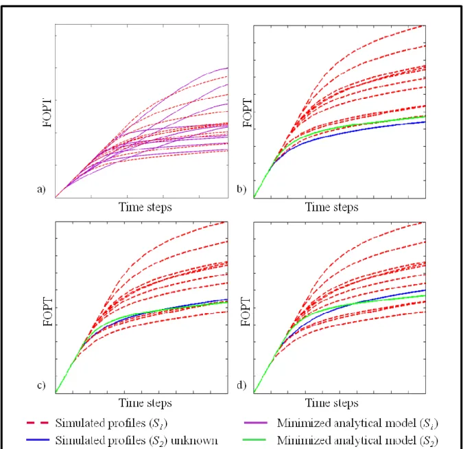
6a shows that the ranking of the estimated analytical curves is the same as the reference ranking for

27

most time steps (especially for long simulation times). However, some rank inversions are visible for 28

intermediate time steps. Also, the linear part of the obtained production curves is often too short as 29

compared to the true profiles. This could be due to the relatively small number of samples, or to the 30

existence of local minima in the non-linear optimization. To reduce these errors we propose an 31

optional kriging-based correction method described in Appendix. 32

We then ran the non-linear minimization of Eq. (10) for all the models of based on the distance to 33

all ten models of set ( ). To speed up this optimization, we selected as starting point of the 34

minimization the parameters of the known curve for which the objective function value was lowest. 35

(14)

13 Three individual comparisons between the estimated analytical profiles and the true profiles from the 1

reference simulations are presented in Fig. 6b-d. In these cases, also, the analytical profiles are 2

correlated to the reference ones, but display some variations. We think these deviations occur partly 3

because of errors in the proxy-based distances and partly because distances are unable to uniquely 4

characterize the shape of the production curves. Further research is needed to characterize these 5

sources of error and to characterize the numerical properties of the minimization of Eq (10). 6

7

Fig. 6 – (a) Minimization of the analytical model parameters for the models belonging to , dashed curves correspond 8

to the reference profiles obtained with a full physics flow simulator and the purple ones are obtained after 9

minimization. (b-d) Examples of minimization procedure results. Red dashed curves correspond to the real response 10

profile of models belonging to , green curves to the analytical curve of a model belonging to and blue curves to 11

corresponding real profile (computed with full physics flow simulator and not known in operational context). 12

9 Production curve quantiles and confidence intervals

13

The above procedures produce a set of true production profiles (from flow simulation on models 14

belonging to ) and estimated analytical profiles (from the minimization of Eq. (10) on 15

all models of ). The corresponding curves are shown on Fig. 7a. For each time step, we create a 16

(15)

14 discrete probability distribution function from these profiles. Final surrogate quantile curves are 1

obtained by linking the quantiles of these distributions across all the time steps. 2

Fig. 7b shows the results of quantile curves estimation for our case study. The curves estimated with

3

our methodology are closer to the reference than the production profiles of the models in . This 4

confirms experimentally that proxies integrated with the proposed method reduce uncertainty 5

quantification errors as compared to uncertainties estimated only from a few representative models. 6

However, the errors discussed in Section 8 are still visible when comparing the computed quantiles 7

and the reference quantiles obtained from flow simulation on all models. In particular, the Q10 and 8

Q50 curves underestimate the time when production starts declining, yielding more conservative 9

production scenarios. 10

11

Fig. 7 – Final analytical production curves and corresponding quantiles (a) Analytical curves obtained after 12

minimization applied to each model of (full green lines) and accurate curves obtained by flow simulation on 13

models (dashed red lines). (b) Quantiles (Q10 in blue, Q50 in black and Q90 in red) computed with all models ( ) 14

(reference, dashed lines); quantiles computed only with models belonging to (doted lines); quantiles computed with 15

our methodology ( ) (full lines). (c) Minimized profiles after correction (see Appendix). (d) Quantiles updated with 16

corrected profiles for our methodology (full lines). 17

To remove these systematic errors, we applied the correction described in Appendix. As shown on 18

Fig. 7c, this correction introduces some non-admissible behaviors in individual curves. For instance,

19

some cumulative production curves locally have a negative slope. However, these local 20

inconsistencies are filtered by the quantile estimation process and the final quantile curve estimates 21

(Fig. 7d) are closer to the reference curves. 22

(16)

15 In all cases, quantile curve estimations are prone to several sources of uncertainty. First, there is no 1

guarantee about the representativeness of the subset of models selected for full flow simulation. 2

This could ideally be addressed by increasing the number of models in until the output statistics 3

converge. Because this can be computationally infeasible, another option is to repeat the k-medoid 4

clustering process (Section 5) starting from different initial models. Indeed, the k-medoid algorithm is 5

sensible to the choice initial models, as mentioned by Josset and Lunati (2013). This option is 6

computationally expensive but can provide a practical way to assess confidence intervals around the 7

quantile curves for a fixed number of models in . 8

A second source of uncertainty relates to the nature of the chosen proxy which, as the name suggests, 9

only approximates the actual flow response. Indeed, more accurate proxies should in principle lead to 10

better confidence in the quantile curve estimates. In our method, this proxy error is sampled during the 11

missing distance reconstruction (Section 6). Resampling alternative distances from the piecewise 12

regression model provides an efficient way to address this source of uncertainty without need for 13

additional flow simulations. 14

In this study, we first applied our methodology 200 times. Due to the stochasticity of the k-medoid 15

algorithm used in the DKM (Section 5), we were able to generate 200 different sets of quantile profiles 16

(Q10, Q50 and Q90) and then computed the confidence interval around them with ten representative 17

models (Fig. 8a). The confidence intervals obtained with our method do not always include the actual 18

quantile curves generated from the reference simulations due to proxy error or workflow limitations. 19

We suspect that the correction step described in the appendix could explain why these confidence 20

intervals are too low. Indeed, this correction may artificially lower the profiles. Therefore, we chose to 21

increase the number of representative models to twenty and ran the randomized workflow 200 times to 22

obtain new confidence intervals (Fig. 8b). The results in this case are better in the sense that 23

confidence intervals are slightly narrower and include the reference quantile curves. In contrast, we 24

applied 200 random selections of representative models, and aggregated the true production curves to 25

compute the associated confidence intervals (Fig. 8c). When our methodology is used, the confidence 26

intervals are narrower due to the integration of proxy knowledge. 27

28

Fig. 8 – Quantiles dispersion over 200 iterations of the methodology. (a) With a subset of 10 models. (b) With a 29

subset of 20 models. (c) With 10 models in but without using proxies from in the quantile computation. 30

10 Conclusions

31

Estimating the uncertainties on the flow response of a reservoir by performing full physics flow 32

simulation on a large ensemble of models implies often prohibitive simulation time. To overcome this 33

(17)

16 problem, some approaches consider an approximation of the dynamic simulation response which is 1

obtained faster by simplification of the physics of the simulator. The use of these proxies leads to a 2

delicate issue of balancing acceleration with accuracy of the response. Another problem is that proxies 3

are very often case-dependent; choosing the proxy which is best suited to a given case study can be a 4

long procedure (Bardy et al. 2014). Other approaches consider selecting only a few models from the 5

initial set and run the accurate flow simulation only on this small subset. Our approach aims at 6

integrating the dynamic behavior of the whole set of models to capture the uncertainties, as also 7

proposed by Josset and Lunati (2013). The method proposed in this paper allows for a larger class of 8

proxies to be considered, but it calls for the explicit definition of analytical production profiles, which 9

depend on the type of reservoir simulation output. From a reservoir management standpoint, it could 10

be interesting to use other types of production curves such as water production or pressure, because it 11

can also be important to adjust surface facilities. Looking at the well by well response would also be 12

important as this is where proxies lack accuracy. Applying this methodology to any other kind of 13

curve like water profile is possible but relies on the availability of compact analytical models for the 14

considered reservoir response curve. 15

In this paper, the model selection was performed using the Distance Kernel Method (Scheidt and 16

Caers, 2009) but other selection techniques could be considered. For field development studies, further 17

research is also needed to assess how to address more complex development scenarios where multiple 18

well locations are considered and well schedule changes though time. 19

Nonetheless, the results obtained show that the methodology can assess reservoir oil production 20

uncertainty even with a very simple proxy. It would be interesting to assess the value of this method to 21

accelerate history matching tasks in the same spirit as Scheidt et al (2011) and Josset et al. (2015). It 22

would also be interesting to test this methodology on a case study where the full flow simulation 23

responses are more chaotic and with a less regular dispersion. 24

Acknowledgments

25

The authors of this paper, would like to thank Total S.A. for funding this research and providing the 26

case study, Celine Scheidt for providing the initial distance kernel method code, as well as Peter King 27

(Imperial College) and Vicent Corpel (Total S.A) for their unconditioned help. We also thank Pedram 28

Masoudi, and the other reviewers whose comments helped us to improve this paper. 29

References

30

Abrahamsen, P., 1993, Bayesian kriging for seismic depth conversion of a multi-layer

31

reservoir, in Geostatistics Troia’92: Springer, p. 385–398.

32

Alabert, F.G., Modot, V., 1992. Stochastic Models of Reservoir Heterogeneity: Impact on

33

Connectivity and Average Permeabilities, in: SPE Annual Technical Conference and

34

Exhibition. Society of Petroleum Engineers, Washington, D.C. doi:10.2118/24893-MS

35

Ballin, P.R., Journel, A.G., Aziz, K., 1992. Prediction Of Uncertainty In Reservoir

36

Performance Forecast. J Can Pet Tech 31. doi:10.2118/92-04-05

37

Bardy, G., 2015. Intégration de modèles approchés pour mieux transmettre l’impact des

38

incertitudes statiques sur les courbes de réponse des simulateurs d’écoulements. PhD Thesis,

39

Université de Lorraine.

40

Bardy, G., Biver, P., Caumon, G., Renard, P., Corpel, V., King, P.R., 2014. Proxy

41

Comparison for Sorting Models and Assessing Uncertainty on Oil Recovery Profiles, in:

(18)

17

ECMOR XIV - 14th European Conference on the Mathematics of Oil Recovery. EAGE.

1

doi:10.3997/2214-4609.20141901

2

Caers J (2011) Modeling Uncertainty in the Earth Sciences. Wiley-Blackwell,

3

Corre, B., Thore, P., de Feraudy, V., Vincent, G., 2000. Integrated Uncertainty Assessment

4

For Project Evaluation and Risk Analysis, in: SPE European Petroleum Conference. Society

5

of Petroleum Engineers, Paris, France. doi:10.2118/65205-MS

6

Cox, T.F., Cox, M.A., 2001. Multidimensional scaling, 2nd ed, Monographs on statistics and

7

applied probability. Chapman & Hall/CRC press.

8

Deutsch, C.V., 1998. Fortran programs for calculating connectivity of three-dimensional

9

numerical models and for ranking multiple realizations. Computers & Geosciences 24, 69–76.

10

doi:10.1016/S0098-3004(97)00085-X

11

Doherty, J., Christensen, S., 2011. Use of paired simple and complex models to reduce

12

predictive bias and quantify uncertainty. Water Resources Research 47, n/a-n/a.

13

doi:10.1029/2011WR010763

14

Durlofsky LJ, 2005. Upscaling and gridding of fine scale geological models for flow

15

simulation. In: 8th International Forum on Reservoir Simulation, Stresa, Italy, 2005.

16

Fenwick, D., Scheidt, C., Caers, J., 2014. Quantifying Asymmetric Parameter Interactions in

17

Sensitivity Analysis: Application to Reservoir Modeling. Mathematical Geosciences 46, 493–

18

511. doi:10.1007/s11004-014-9530-5

19

Fetel, E., Caumon, G., 2008. Reservoir flow uncertainty assessment using response surface

20

constrained by secondary information. Journal of Petroleum Science and Engineering 60,

21

170–182. doi:10.1016/j.petrol.2007.06.003

22

Fetkovich, M.J., Fetkovich, E.J., Fetkovich, M.D., 1996. Useful Concepts for Decline Curve

23

Forecasting, Reserve Estimation, and Analysis. SPE Reservoir Engineering 11, 13–22.

24

doi:10.2118/28628-PA

25

Ginsbourger, D., Rosspopoff, B., Pirot, G., Durrande, N., Renard, P., 2013. Distance-based

26

kriging relying on proxy simulations for inverse conditioning. Advances in Water Resources

27

52, 275–291. doi:10.1016/j.advwatres.2012.11.019

28

Gross, H., 2012. Response surface approaches for large decision trees: decision making under

29

uncertainty, in: ECMOR XIII-13th European Conference on the Mathematics of Oil

30

Recovery. doi:10.3997/2214-4609.20143195

31

Hovadik, J., Larue, D., 2011. Predicting waterflood behavior by simulating earth models with

32

no or limited dynamic data: From model ranking to simulating a billion-cell model, in:

33

Uncertainty Analysis and Reservoir Modeling, AAPG Memoir. pp. 29–55.

34

doi:10.1306/13301406M961028

35

Josset, L., Lunati, I., 2013. Local and Global Error Models to Improve Uncertainty

36

Quantification. Mathematical Geosciences 45, 601–620. doi:10.1007/s11004-013-9471-4

37

Josset, L., Ginsbourger, D., Lunati, I., 2015a. Functional error modeling for uncertainty

38

quantification in hydrogeology. Water Resources Research 51, 1050–1068.

39

doi:10.1002/2014WR016028

40

Josset, L., Demyanov, V., Elsheikh, A.H., Lunati, I., 2015b. Accelerating Monte Carlo

41

Markov chains with proxy and error models. Computers & Geosciences 85, 38–48.

42

doi:10.1016/j.cageo.2015.07.003

(19)

18

Kaufman, L., Rousseeuw, P., 1987. Clustering by means of medoids. North-Holland.

1

Majdi Yazdi, M., Jensen, J.L., 2014. Fast screening of geostatistical realizations for SAGD

2

reservoir simulation. Journal of Petroleum Science and Engineering 124, 264–274.

3

doi:10.1016/j.petrol.2014.09.030

4

Manceau, E., Zabalza-Mezghani, I., Roggero, F., 2002. Use of experimental design

5

methodology to make decisions in an uncertain reservoir environment from reservoir

6

uncertainties to economic risk analysis, in: 17th World Petroleum Congress, Rio de Janeiro,

7

Brazil.

8

Maschio, C., de Carvalho, C.P.V., Schiozer, D.J., 2010. A new methodology to reduce

9

uncertainties in reservoir simulation models using observed data and sampling techniques.

10

Journal of Petroleum Science and Engineering 72, 110–119. doi:10.1016/j.petrol.2010.03.008

11

Maschio, C., Schiozer, D.J., 2014. Bayesian history matching using artificial neural network

12

and Markov Chain Monte Carlo. Journal of Petroleum Science and Engineering 123, 62–71.

13

doi:10.1016/j.petrol.2014.05.016

14

Nocedal, J., Wright, S.J., 2006. Numerical optimization, 2nd edn., Springer series in

15

operations research. Springer, New York.

16

Obi, E., Eberle, N., Fil, A., Cao, H., 2014. Giga Cell Compositional Simulation, in:

IPTC-17

17648-MS. Presented at the International Petroleum Technology Conference, Doha, Qatar.

18

doi:10.2523/IPTC-17648-MS.

19

Rahim, S., Li, Z., Trivedi, J., 2015. Reservoir Geological Uncertainty Reduction: an

20

Optimization-Based Method Using Multiple Static Measures. Mathematical Geosciences 47,

21

373–396. doi:10.1007/s11004-014-9575-5

22

Renard, P., Allard, D., 2013. Connectivity metrics for subsurface flow and transport.

23

Advances in Water Resources 51, 168–196. doi:10.1016/j.advwatres.2011.12.001

24

Scheidt, C., Caers, J., 2009. Representing Spatial Uncertainty Using Distances and Kernels.

25

Mathematical Geosciences 41, 397–419. doi:10.1007/s11004-008-9186-0

26

Scheidt, C., Caers, J., 2010. Bootstrap confidence intervals for reservoir model selection

27

techniques. Computational Geosciences 14, 369–382. doi:10.1007/s10596-009-9156-8

28

Scheidt, C., Caers, J., Chen, Y., Durlofsky, L.J., 2011. A multi-resolution workflow to

29

generate high-resolution models constrained to dynamic data. Computational Geosciences 15,

30

545–563. doi:10.1007/s10596-011-9223-9

31

Scheidt, C., Li, V., Caers, J., 2018. Bayesian Evidential Learning, in: Quantifying Uncertainty

32

in Subsurface Systems, Geophysical Monograph Series. John Wiley & Sons, Inc., Hoboken,

33

NJ, USA, pp. 193–215. https://doi.org/10.1002/9781119325888.ch7

34

Schiozer, D.J., Ligero, E.L., Suslick, S.B., Costa, A.P.A., Santos, J.A.M., 2004. Use of

35

representative models in the integration of risk analysis and production strategy definition.

36

Journal of Petroleum Science and Engineering 44, 131–141. doi:10.1016/j.petrol.2004.02.010

37

Subbey, S., Christie, M., Sambridge, M., 2004. Prediction under uncertainty in reservoir

38

modeling. Journal of Petroleum Science and Engineering 44, 143–153.

39

doi:10.1016/j.petrol.2004.02.011

(20)

19

Suzuki, S., Caers, J., 2008. A Distance-based Prior Model Parameterization for Constraining

1

Solutions of Spatial Inverse Problems. Mathematical Geosciences 40,445-469.

2

doi:10.1007/s11004-008-9154-8

3

Suzuki, S., Caumon, G., Caers, J., 2008. Dynamic data integration for structural modeling:

4

model screening approach using a distance-based model parameterization. Computational

5

Geosciences 12, 105–119. doi:10.1007/s10596-007-9063-9

6

Thiele, M.R., Batycky, R.P., Blunt, M.J., Orr Jr, F.M., 1996. Simulating flow in

7

heterogeneous systems using streamtubes and streamlines. SPE Reservoir Engineering 11, 5–

8

12. doi:10.2118/27834-PA

9

Wang, K., Liu, H., Chen, Z., 2015. A scalable parallel black oil simulator on distributed

10

memory parallel computers. Journal of Computational Physics 301, 19–34.

11

doi:10.1016/j.jcp.2015.08.016

12

Xie, J., Yang, C., Gupta, N., King, M.J., Datta-Gupta, A., 2015. Integration of

Shale-Gas-13

Production Data and Microseismic for Fracture and Reservoir Properties With the Fast

14

Marching Method. SPE-161357-PA 20, 347–359. doi:10.2118/161357-PA

15

Zabalza-Mezghani, I., Manceau, E., Feraille, M., Jourdan, A., 2004. Uncertainty management:

16

From geological scenarios to production scheme optimization. Journal of Petroleum Science

17

and Engineering 44, 11–25. doi:10.1016/j.petrol.2004.02.002

18 19 20

(21)

20

11 Appendix: Error correction

1

We propose an optional correction stage to reduce the errors between the surrogate curves and the true 2

curves. This correction makes the assumption that errors have zero mean, are smooth, and can be 3

characterized only from the models of set . It is similar in spirit to the “gobal error model” 4

introduced by Josset and Lunati (2013), but it considers production profiles instead of breakthrough 5

curves and uses time-dependent weighting instead of a global distance-based weighting. This 6

correction takes the form of a vertical shift map (Section 8), computed as follows: 7

- For every known model (belonging to ) the difference between the true profile and the 8

reconstructed one is computed (Fig. 9a). 9

- These differences are projected on the analytical curves in the plot space (Fig. 9b) 10

- The differences are then interpolated for each time step using simple kriging with a 0 mean. 11

The juxtaposition of all the 1D corrections over all the time steps covers the entire domain 12

FOPT versus time (Fig. 9c). 13

The final corrected production profiles are finally obtained by subtracting the error estimate from the 14

reconstructed analytical profiles. 15

16

Fig. 9 – (a) Error computed between simulation profiles and analytical profile for two models belonging to . (b) 17

Mapping error on analytical model. (c) Interpolation of the error on the entire plot domain to create an error map. 18