1
Textural variants of iron ore from Malmberget:
characterization, comminution and mineral liberation
Pierre-Henri KOCH
Luleå, June 2013
Presented in partial fulfillment of the requirements for the degree of master in Geology and
Mining Engineering
Supervisor: Prof. Pertti Lamberg
Department of Civil, Environmental and Natural Resources Engineering Division of Sustainable Process Engineering
Luleå University of Technology (LTU)
Department ArGEnCo : Architecture, Géologie, Environnement et Constructions Division GeMMe : Génie Minéral, Matériaux et Environnement
3
Abstract
Geometallurgy combines geology and mineral processing into a spatially-based predictive model and is a useful tool that can be used in production management of a mineral processing plant. Two main complementary approaches exist to establish this model. Geometallurgical testing relies on direct measurement of the response of the ore in the processing circuit by conducting several small scale metallurgical tests. The mineralogical approach relies on proper ore characterization and process modeling on mineral basis. Because the latter is generic and applicable to any type of mineral deposit, it was chosen as the main basis of this study and combined with rock mechanics as basic geometallurgical testing.
This work presents comminution characterization of different textural variants of the breccia (semi-massive) iron ore from Malmberget, Northern Sweden. Experimental work includes Point Load Tests, Compressive Tests, comminution as laboratory crushing and grinding, mineralogical characterization and liberation measurements of the products. The results give quantitative information on how physical properties, modal mineralogy and mineral textures are related to comminution and mineral liberation. This work is directly linked with three on-going Ph.D. projects at LTU and contributes to a framework on how mineral textures and liberation information can be included in a geometallurgical model.
4
Abstract (Swedish)
Geometallurgi kombinerar geologi och mineralprocesser i en prediktiv rumsligt-baserad modell. Det är ett användbart verktyg som kan användas i produktionsstyrningen vid anriknings- och metallurgiska processer. Huvudsakligen finns det två metoder för att utveckla denna modell. De geometallurgiska testerna, förlitar sig på den direkta metallurgiska responsen som malmen ger från flera småskaliga metallurgiskatester. Det mineralogiska tillvägagångssättet bygger på en korrekt malmkarakterisering och process modellering av fyndighetens kvantitativa mineralogi. Eftersom den senare är mer allmän och är tillämpningsbar för de flesta malmfyndigheterna, valdes den i denna studie.
I detta master arbete presenteras en kross- malbarhetens karakterisering av olika texturella varianter av en malm breccia (semi-massiv malm), från Malmberget apatitjärn fyndighet i norra Sverige. Det experimentella arbetet består utav punktlast-tester, tryckprovning, laborationer, krossning och malningstester med tillhörande frimalningsmätningar av de olika produkterna. Resultatet ger en kvantitativ information om de fysiskaliska egenskaperna, den modala mineralogin och hur mineral texturerna är relaterade till malbarhet och frimalning av olika mineral. Detta arbete är direkt sammankopplat med tre pågående doktorandprojekt vid Luleå Tekniska universitet och bidrar till en struktur om hur information om mineraltexturer och frimalning kan ingå i en geometallurgical modell.
5
Preface
This is the final report of the master thesis “Textural variants of iron ore from Malmberget : characterization, comminution and mineral liberation“ started in January 2013 and finished in June 2013 at Luleå University of Technology in Luleå, Sweden in the division of Sustainable Process Engineering of Luleå tekniska universitet (LTU), supervised by Prof. Pertti Lamberg. A presentation of this work has been done the 6 of June 2013 at LTU and the 14 of June in Koskullskulle (Malmberget) Research Center for LKAB.
Luossavaara-Kiirunavaara Aktiebolag (LKAB) is gratefully acknowledged for funding this work, providing samples, X-Ray fluorescence analysis and help.
This work would not have been possible without the help and assistance of • Prof. Pertti Lamberg (LTU), supervisor
• Prof. Jan Rosenkranz (LTU), examiner • Abdul Mwanga (LTU) PhD, co-supervisor • Cecilia Lund (LTU) PhD, co-supervisor
• Therese Lindberg (LKAB), Geometallurgy@LKAB • Prof. Eric Pirard (ULg), home university supervisor
6
Table of content
Abstract ... 3 Abstract (Swedish) ... 4 Preface ... 5 Table of figures ... 7 1. Introduction ... 10 a. Regional geology ... 10 b. Deposit geology ... 12c. Mineralogy and chemistry of the ore ... 13
2. Objectives and working hypothesis ... 17
3. Literature review ... 18
a. Geometallurgy ... 18
b. Physical properties and rock mechanics ... 20
c. Comminution testing ... 24
d. Liberation analysis using Scanning Electron Microscope (SEM)... 25
e. XRF Analysis and Element to Mineral conversion ... 28
f. Liberation models ... 29
4. Experimental work ... 32
a. Classification of samples ... 32
b. Rock mechanics material and methods ... 36
c. Comminution material and method ... 37
d. XRF analysis and element-to-mineral conversion material and method ... 37
e. SEM liberation material and method ... 39
f. Liberation model by archetypes material and method ... 41
5. Results ... 44
a. Rock mechanics analysis ... 44
b. Comminution analysis ... 51
c. Liberation analysis ... 53
d. Empirical linear models ... 65
6. Summary and conclusion ... 71
7. Limitations of the study and further work ... 72
8. References ... 73
9. Appendices ... 79
a. Appendix A: additional figures ... 79
7
Table of figures
Figure 1 : Main events and series in the northern Norrbotten province (Bergman, Kübler, & Martinsson,
2001), not to scale. ... 11
Figure 2 : Geological map of Malmberget area (Lund, Andersen, & Martinsson, 2009, modified) ... 12
Figure 3 : 3D view of Fabian and Printzsköld ore bodies (LKAB, 2013), modified ... 13
Figure 4 : Typical chemical composition of Fabian ore ... 14
Figure 5 : Typical chemical composition of Fabian ore breccia ... 15
Figure 6 : Typical chemical composition of Printzsköld ore ... 16
Figure 7 : Typical chemical composition of Printzsköld ore breccia ... 16
Figure 8 : General geometallurgical program of this work (Lamberg 2011), modified. ... 20
Figure 9 : Different configurations for the Point Load Test (Bieniawski 1975) ... 22
Figure 10 : Typical setting for simple compressive test, (Shosha 2013) ... 23
Figure 11 : XRF and EDS simplified mechanism (CLU-IN 2013) ... 26
Figure 12 : BSE simplified mechanism (Dewar 2013), modified ... 26
Figure 13 : Relation between mean grey level and atomic number at constant brightness and contrast (Schneider 2004) ... 27
Figure 14 : Data structures used to classify the samples ... 32
Figure 15 : Samples classification system (Lund 2013), modified ... 33
Figure 16 : Sample preparation for CF1 ... 34
Figure 17 : Name, description and pictures of feldspar breccia samples CF1 to CF8 (Lund 2013)... 35
Figure 18 : PLT validity criterion adapted to non-standard samples ... 36
Figure 19 : Merlin SEM column schematic (Zeiss 2011) ... 39
Figure 20 : Simple example of association index (AI) ... 43
Figure 21 : normal probability plot for PLT values of the whole population ... 44
Figure 22 : Is(50) mean values and 95 % CI bars for CF1 to CF8 ... 45
Figure 23 : Correlation between Is(50) and compressive strength ... 46
Figure 24 : Compressive strength mean values and 95 % CI bars for CF1 to CF8 ... 47
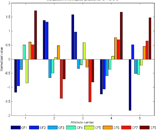
Figure 25 : Comparison of normalized attributes for samples CF1 to CF8 ... 50
Figure 26 : Classification of the samples into three clusters ... 51
Figure 27 : Lin-log sieving curve for comminution steps ... 52
Figure 28 : Magnetite content in weight measured by the SEM compared to its EMC measurement ... 54
Figure 29 : Specific gravity measurement with 95 % CI ... 54
Figure 30 : Specific gravity measured by the SEM compared to its EMC measurement ... 55
Figure 31 : Modal mineralogy in size fraction 53-75 µm ... 56
Figure 32 : Magnetite versus apatite, albite, tremolite and orthoclase contents in weight in size fractions of the samples. ... 57
Figure 33 : Mode of occurrence of magnetite in CF2 with interpolated data ... 58
Figure 34 : Cumulative liberation curve of magnetite in CF2 for all size fractions with interpolated data 59 Figure 35 : Mode of occurence of magnetite in size fraction 53-75 µm for all samples classes ... 60
Figure 36 : Initial AI for magnetite as target mineral ... 62
Figure 37 : CRC rebalanced AI for magnetite as target mineral ... 63
Figure 38 : CRF rebalanced AI for magnetite as target mineral ... 63
Figure 39 : CF4 rebalanced AI for magnetite as target mineral ... 64
8
Figure 41 : Predicted versus measured values for model 2 ... 67
Figure 42 : Predicted versus measured values for model 3 ... 68
Figure 43 : Predicted versus measured values for model 4 ... 69
Figure 44 : Predicted versus measured values for model 5 ... 70
Figure 45 : Geological map of northern Norrbotten county, Sweden (Bergman 2001) ... 79
Figure 46 : Malmberget's mine plan (LKAB 2011)... 80
Figure 47 : Compressive strength of CF1 and CF2 samples ... 80
Figure 48 : Compressive strength of CF3 and CF4 samples ... 81
Figure 49 : Compressive strength of CF5 and CF6 samples ... 81
Figure 50 : Compressive strength of CF7 and CF8 samples ... 82
Figure 51 : Compressive strength of CRC and CRF samples ... 82
Figure 52 : Is(50) of CF1 and CF2 samples ... 83
Figure 53 : Is(50) of CF3 and CF4 samples ... 83
Figure 54 : Is(50) of CF5 and CF6 samples ... 84
Figure 55 : Is(50) of CF7 and CF8 samples ... 84
Figure 56 : Is(50) of CRC and CRF samples ... 85
Figure 57 : General clustering process (Mooi 2011) ... 85
Figure 58 : Jaw crusher (left) and Ball mill (right) used in this work ... 86
Figure 59 : Modal composition of CF4 and CF6 for the 53-75 µm size fraction ... 86
Figure 60 : Mode of occurrence of magnetite in CF2 ... 87
Figure 61 : Cumulative liberation curve of magnetite in CF2 ... 87
Figure 62 : Mode of occurrence of magnetite in CF4 ... 88
Figure 63 : Cumulative liberation curve of magnetite in CF4, ... 88
Figure 64 : Mode of occurrence of magnetite in CF6 ... 89
Figure 65 : Cumulative liberation curve of magnetite in CF6 ... 89
Figure 66 : Mode of occurrence of magnetite in CRC ... 90
Figure 67 : Cumulative liberation curve for magnetite in CRC ... 90
Figure 68 : Mode of occurrence of magnetite in CRF ... 91
9
Table 1 : Sample material properties and number of valid mechanical tests per class ... 37
Table 2 : Settings for the element to mineral conversion ... 38
Table 3 : Standardized attributes matrix ... 49
Table 4 : Computation of the reduction ratio for comminution steps (f80 for feed and p80 for product) 53 Table 5 : Degree of liberation of magnetite, i.e. mass proportion of fully liberated magnetite ... 61
Table 6 : Similarities between classes ... 64
Table 7 : Data used to build the models ... 65
Table 8 : Model 1 values and error ... 66
Table 9 : Model 2 values and error ... 67
Table 10 : Model 3 values and error ... 68
Table 11 : Model 4 values and error ... 69
Table 12 : Model 5 values and error ... 70
Table 13 : Composites and samples ... 92
Table 14 : PLT and CS measurements for all samples ... 92
Table 15 : Correction factor for the laboratory ball mill ... 98
Table 16: MERLIN scanning electron microscope specification sheet (Zeiss 2011) ... 99
Table 17 : Microprobe analysis of magnetite and ilmenite of Fabian ore body (Lund et al., 2009) ... 100
Table 18 : Microprobe analysis of magnetite and ilmenite from Fabian ore breccia (Lund et al., 2009) 100 Table 19 : statistics and t-test for magnetite between SEM and EMC ... 101
Table 20 : statistics and t-test for specific gravity between SEM and EMC ... 101
Table 21 : Statistics for model 1 ... 102
Table 22 : Statistics for model 2 ... 102
Table 23 : Statistics for model 3 ... 103
Table 24 : Statistics for model 4 ... 104
10
1. Introduction
Malmberget is a large iron ore mine located in northern Sweden (Norrbotten County) operated by LKAB. The deposit has proven reserve of 174 million tons (Mt) at 42.4 % Fe (probably 105 Mt at 41.2 % Fe) and mineral assets besides mineral reserves of 21 Mt measured at 48.9 % Fe , 175 Mt indicated at 45.7 % Fe and 30 Mt inferred at 44.2 % Fe (LKAB 2011). The total size of the deposit is estimated to 840 Mt at 51 to 61 % Fe (Weiheid P 2008).
The total number of iron deposits in northern Norrbotten is about 40, with an iron grade ranging from 30 to 70 %, varying magnetite/hematite ratio, a phosphorus content between 0.05 and 5 and in most of them show strong LREE and moderate Th enrichment.
To enable more effective utilization of the ore body and production management, LKAB is evaluating the feasibility of a geometallurgical program in Kiruna (Niiranen et al. 2012) and Malmberget (Lund et al., in prep)
a. Regional geology
The oldest rocks of the Norrbotten province belong to Archean basement (granitoid-gneiss) ending with intrusive tonalite-granodiorite (2.8 Ga). This first group has been intruded by multiple groups of dykes (mafic).
On top of it comes the Kovo Group (2.5 – 2.3 Ga) ranging from clastic sediments to volcanic rocks in a context of a rift. The following group is the Kiruna Greenstones consisting of a base layer of komatiites and basalts, a middle layer of carbonates and volcaniclastic sediments and the end term with MORB-type lava (Martinsson 1997, Martinsson 2004). This sequence underwent metamorphism and deformation during the Svecokarelian orogen (1.9–1.8 Ga).
The Haparanda Suite is an early orogenic rock series that contains calc-alkaline volcanic rocks dated to 1.9 – 1.88 Ga (Öhlander 1984, Weihed, Arndt et al. 2005). The next sequence is the Perthite monzonite suite (chemically similar to the Kiirunavaara Group and dated from 1.88 to 1.86 Ga) which consists of more alkaline magmatic rocks. Malmberget deposit is linked to the Porphyry Group (cf. Figure 1) and the Kiruna deposit both in space and time with a genesis dated from 1.88 Ga (Romer 1994). From 1.81 to 1.78 Ga, the Lina suite intrusions displayed a magmatic activity linked to the Svencofennian orogen by
11
the fusion of parts of the middle crust (Weihed, Arndt et al. 2005). A simplified view of these series and events is presented on Figure 1.
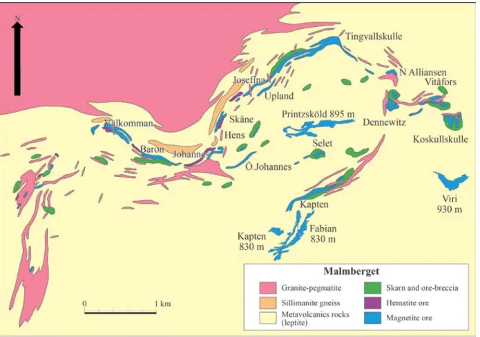
12 b. Deposit geology
The Malmberget deposit consists of more than 20 iron ore bodies of varying mineralogy. Characteristic for Malmberget is the deformed and metamorphosed nature of the host rocks. Ductile deformation and at least two phases of folding produced the ore lenses, many of which exhibit boudinaged structures along the dipping direction (Bergman 2001). Figure 2 shows the geological setting of the ore in Malmberget with the names of the different ore bodies.
Figure 2 : Geological map of Malmberget area (Lund, Andersen, & Martinsson, 2009, modified)
Iron ore can be divided into massive ore (stratiform-stratabound) and ore breccia (Geijer 1930). The ore breccia is defined as “an irregular network of ore veins which to a varying extent accompany the massive ore” (Geijer 1930, Frietsch 1982). A more generic term semi-massive ore is also used (Lund, in prep). According to (Lund 2009), the massive ore formation can be due to either high temperature hydrothermal fluid circulation or to an iron-enriched magma, whereas the ore breccia mineralization could be caused by low temperature hydrothermal fluid circulation like in the formation of IOCG deposits. The ore breccia samples used in this study cover the Fabian (Fa) and Printzsköld (Pz) ore
13
bodies as shown on figure 2 and 3. Reference samples of ore come from Hens ore body displayed on figure 2 .
Figure 3 : 3D view of Fabian and Printzsköld ore bodies (LKAB, 2013), modified
c. Mineralogy and chemistry of the ore i. Fabian magnetite ore
Based on the difference established previously between ore and ore breccia, this section distinguishes between the center of Fabian (ore) and the breccia-style mineralization (ore breccia) that surrounds it.
1. Fabian ore
In Fabian ore, the main iron-containing minerals are
• Magnetite (Mgt) : mineral of the spinel group with chemical formula Fe2+Fe3+ 2O4
• Ilmenite (Il) : mineral of the ilmenite group with chemical formula Fe2+TiO 3
It must be noticed that hematite also exists but does not dominate. Figure 4 shows the whole rock chemical analysis according to data obtained by Cecilia Lund.
14
Figure 4 : Typical chemical composition of Fabian ore
Chemical compositions of the main iron containing minerals analyzed by Lund (2012) with electron microprobe are given in Appendix B. The iron (Fe) content in Fabian ore magnetite ranges from 70 % to 72% irrespective of grain size whereas in ilmenite, the total iron content is 42 %.
2. Fabian ore breccia
According to (Lund 2009), the gangue minerals that form the silicate matrix in the breccia ore are albitic plagioclase with K-feldspar and quartz. The iron containing minerals are magnetite and small amounts of Ilmenite. Other minerals include amphibole, pyroxene, biotite, pyrite, anhydrite chalcopyrite and zircon. Figure 5 shows typical chemical composition of ore breccia.
9.24% 0.89%
80.99% 0.08%
2.29% 3.80%
0.51% 0.11% 1.64% 0.45%
Representative composition in major elements of the
whole rock for Fabian ore
SiO2 Al2O3 Fe2O3 MnO MgO CaO Na2O K2O TiO2 P2O5
15
Figure 5 : Typical chemical composition of Fabian ore breccia
Regarding the content of the main iron containing minerals, the microprobe results show a different situation than in the massive ore. Overall, in the breccia ore the ore magnetite is richer in traces elements as seen on table in the Appendix. The fact that the gangue minerals as well as the trace elements in magnetite differs between the massive ore and the ore breccia may indicate a different origin as discussed previously in section 1.b. (Lund 2009)
ii. Printzsköld ore body
1. Printzsköld ore
In Printzsköld ore, the main iron minerals are
• Magnetite (Mgt) : mineral of the spinel group with chemical formula Fe2+Fe3+ 2O4
• Hematite (Hm) : mineral of the hematite (or corundum) group with chemical formula Fe2O3
Figure 6 presents a representative composition of Printzsköld ore.
27.33% 6.15% 56.60%
0.04% 2.36%
3.32% 3.26% 0.09% 0.84% 0.02%
Representative composition of the whole rock for Fabian
ore breccia
SiO2 Al2O3 Fe2O3 MnO MgO CaO Na2O K2O TiO2 P2O516
Figure 6 : Typical chemical composition of Printzsköld ore
2. Printzsköld ore breccia
At the hanging wall contact of Printzsköld, ore breccia presents albitisation and includes biotite, anhydrite and amphiboles. At the footwall contact, ore breccia with massive magnetite has been observed that contains biotite and displays some feldspar, amphiboles, pyroxenes as patches (Debras 2010). Figure 7 presents a representative composition of Printzsköld ore breccia.
Figure 7 : Typical chemical composition of Printzsköld ore breccia
iii. Relation between ore bodies
3.27% 0.30% 77.99% 0.06% 1.45% 9.59% 0.18% 0.05% 0.22% 6.90%
Representative composition in major elements of the
whole rock for Printzsköld ore
SiO2 Al2O3 Fe2O3 MnO MgO CaO Na2O K2O TiO2 P2O5 40.16% 3.97% 42.47% 0.03% 2.26% 4.96% 1.36% 1.56% 0.50% 2.73%
Representative composition in major elements of the
whole rock for Printzsköld ore breccia
SiO2 Al2O3 Fe2O3 MnO MgO CaO Na2O K2O TiO2 P2O5
17
According to Lund et al. (2009), the shift from the oxide mineral association magnetite-ilmenite in Fabian to a magnetite-hematite association in Printzsköld shows the existence of different stages of oxidation from the east (Fabian) to the west, with Printzsköld being intermediate caused by the metamorphic events. The description given by Lund et al (2009) includes both homogeneous magnetite and hematite, as well as homogenous magnetite and ilmenite, and proposes lower stratigraphic position to Fabian and ViRi (for example Kiirunavaara) and a higher position to other orebodies such as Välkomma and Hens. However, the intermediate status of Printzsköld does not allow a clear conclusion despite some indication of a structural move. Another fact supporting this proposed stratigraphy is the trend of the curves V2O5/TiO2 that might indicate a different history of ore bodies (Lund 2009).
2. Objectives and working hypothesis
In a geometallurgical context the geological model must give 3D information on ore properties. It has been proposed that information can be compacted to two terms: modal mineralogy and texture (Lamberg 2011). Lund et al. (in prep) showed that in the case of the felspar-rich breccia ore in Malmberget, textures can be simplified into two main types: fine grained and coarse grained. Accordingly all different textures compose of these two end members.
The purpose of the study is to analyze samples of different textural ore types within the felspar-rich breccia ore, by conducting mechanical and mineralogical characterization on them, carrying outcomminution, creating different size fractions by sieving and measuring the modal mineralogy and liberation spectrum of the product for each size fraction. During the tests, special care is taken regarding the samples, given their limited amount and shape.
This work consists of the following steps:
1. Samples description and specific gravity measurements
2. Geo-mechanical tests on the samples and the first classification (clustering) based on physical properties
3. Comminution (crushing and grinding) of the samples and separation into five different size fractions
4. Elemental analysis of the samples by X-Ray fluorescence (XRF) for each size fraction
5. Liberation and modal mineralogy analysis by scanning electron microscope (SEM) of the samples for selected size fractions
18
6. Use archetypes to describe all the classes and verify the validity of the selected archetypes using the degree of liberation of magnetite and the association index
7. Summarize the characteristics and build predictive empirical models describing all the classes in terms of reduction ratio for jaw crushing, relative work index for ball milling and degree of liberation for magnetite
The hypothesis of the study is that it should be possible to quantitatively describe the textures of
Malmberget feldspar type with two textural archetypes: high graded massive and low graded disseminated.
A definition for the micro texture (micro fabrics) used here has been developed by Lund and Lamberg (in prep): two samples are texturally different if their modally refined liberation distribution is different in a
given particle size.
The motivation of this work is based on the need of the industry to predict the throughput, particle size distribution, modal mineralogy by size fraction and liberation distribution based on modal mineralogy, mineral textures and specific energy. The use of archetypes allows to group different kind of iron ore that are similar in terms of particle size distribution and degree of liberation.
3. Literature review
a. Geometallurgy
In mineral processing, there is a need to take into account geology, mineralogy, processing techniques and metallurgy. To achieve this, McQuiston and Bechaud introduced, as early as 1968, the concept of Geometallurgy : “…geo-metallurgy…since geology is inextricably interwoven with metallurgy in gaining
an understanding of the complexities of a deposit, eventually leading to a definition of mineable reserves, with the development of a flowsheet and engineering criteria for the planning of a successful and profitable operation.” (McQuiston 1968)
The concept can thus be defined as the combination of geological and metallurgical (mineral processing) information to create a spatially-based predictive model for mineral processing plant to be used in production management (Lamberg 2011) or as “the science of integrating geology and mineralogy with
resource processing and extraction” (Hoal 2008).
A geometallurgical program is an industrial application which through different steps leads to a complete geometallurgical model. To achieve this, two approaches should be combined:
19
• Geometallurgical testing: this focuses on the direct measuring metallurgical response of ore samples resulting to a database of parameters that can evaluate how the ore will behave in a treatment plant. This includes a variety of tests in breakage and comminution testing such as JK Bond Ball Lite Test (JKTech, 2013b), Point Load Test, etc or in separation testing, e.g. JKTech Floatability Index (JKFi) (JKTech, 2013a) or Davis tube test (Davis, 1920, 1921).
• Mineralogy (Lamberg 2011): this quantitative approach describes the ore and process based on the minerals. The main hypothesis in the process model is that similar particles ( mineralogy, size, density) will behave in a similar way regardless of their spatial origin within the ore body (Lund 2013).
One difference between these two approaches is the scale at which samples are studied, geometallurgical testing dealing with macroscopic samples whereas mineralogy focuses on particles and minerals at a microscopic scale. Linking the mineralogical with geometallurgical testing into the geometallurgical program is commonly done through statistics and geometallurgical domains, as shown in Figure 8. In this work, the mineralogy approach mixed with some mechanical tests is studied but only the steps involving ore variability testing and the definition of geometallurgical domains are included.
20
Figure 8 : General geometallurgical program of this work (Lamberg 2011), modified.
b. Physical properties and rock mechanics
To gain knowledge about the physical properties of the ore (in-situ or not), several measurements can be done. This section describes briefly in chronological order (from drilling to the lab) some of them that can be used in a geometallurgical program.
First, information can be obtained by doing measurement while drilling (MWD) or Logging While Drilling (LWD). These techniques are usually used in oil and gas industry but can prove useful in many cases since it yields in-situ or close to in-situ measurements of the rock mass. The properties that can be
Plant simulation and validation
Uses the process model with estimated parameters as input Models may be calibrated by benchmarking on existing equipment
Process model
Based on different unit operations Uses parameters previously defined
Estimate parameters over the whole database
Derive mathematical relations from results and apply them
across the dataset Additives properties can be derived from non-additives ones
Define geometallurgical domains
Compare geological ore-type with ore variability results Create domains based on geology and metallurgical response
Ore variability testing
Identify and measure process model parameters Includes characterisation of the ore, comminution testing
Ore sampling
Identify areas of interest based on geological data Sampling for metallurgical testing Collection of geological data
21
measured cover a wide range including gamma ray, induction resistivity , density, neutron porosity, acoustic travel time, pressure sampling, normal and ultrasonic imaging (Trond 2006, Mrozewski 2008). Some information can be gathered from the visual inspection of drill cores by applying a classification of the rock mass (Charlier 2009) :
• Rock quality designation (RQD): measures the recovery from a drill hole. It is given the ratio between the length of the recovered drill core without parts under 100mm in length and the total length of drilling (Deere and Deere 1988). This measurement can be correlated with seismic speeds (in-situ compression and on non-fractured drill core) and the frequency of discontinuities in drilling (Charlier 2009). The resulting information is the quality of rock mass.
• Rock Mass Quality (Q ): extension based on RQD and defined by
𝑄 = �
𝑅𝑄𝐷𝐽 𝑛� �
𝐽𝑟 𝐽𝑎� �
𝐽𝑤 𝑆𝑅𝐹�
(1)
Where RQD is the Rock quality designation, Jn a discontinuity factor, Jr a rugosity factor, Ja a coefficient of alteration in discontinuities, Jw a coefficient accounting for water in discontinuities and SRF a reduction factor based on constraints (Barton N 1974). Based on the value of Q and using tables, the stability and pressures in excavation works can be deduced (Charlier 2009). This information is useful for stability issues but also allows a clearer view of the main weaknesses within the rock mass.
Other classification systems exist that allow more information to be included but are mostly oriented towards stability and tunnel building. Therefore their description is out of the scope of this study but more information can be found in (Charlier 2009).
While rock mechanics tests are usually part of the geometallurgical testing approach, it makes sense to combine both mineralogy and rock mechanics to define geometallurgical domains. Even though, the physical phenomena governing comminution are complex, there is a need to quantify the mechanical properties of the samples. Special interest is provided by the fact that in comminution, a majority of particles are loaded in compression and fail in tension (Briggs and Bearman 1996). A few tests will be described that can be related to the behavior of samples in comminution steps.
• Point Load Test (PLT) : By applying a point load on rock samples and record the breakage pressure, it is possible to get access to the strength of rock materials, particularly the tensile strength (Bieniawski 1975). This test can be conducted on unprepared samples with portable
22
equipment making it a quick and cheap test. Nevertheless, many samples are required to perform statistical analysis on the results. Figure 9 shows the different settings that can be used for this measurement. In this work, only the axial configuration only was used.
Figure 9 : Different configurations for the Point Load Test (Bieniawski 1975)
The measured value at breakage provides Point Load Index (Is) that can be correlated to the tensile strength and compressive strength. Since comminution means breakage, this test seems suitable for ore characterization.
The standard measurement is Is(50), the point load index for an equivalent diameter of 50 mm. This can be linked to the tensile strength given by the Brazilian Test (Charlier 2009) according to
𝐼
𝑠(50) = 0.8𝜎
𝑡𝑏𝑟(2)
Given the anisotropy in rocks, correlation between the point load index and tensile or compressive strength is somehow subject to caution. Whereas earlier works used the following correlation to relate point load index to the compressive strength
𝜎
𝑐= 24 𝐼
𝑠(50)
(3)Where Is(50) is the point load index for a standardized sample size of a 50 mm equivalent diameter. Recent works focus on the study of Is(50) for itself, given that the correlation can vary between 15 to 50 in the case of anisotropic rocks (Charlier 2009). This test is used in this report, a complete description of the test settings and samples can be found under the experimental work section.
• Simple compressive test (CT): The aim of this test is to measure the compressive strength of a rock material. In practice, a sample is placed between two discs of steel while a measured force
23
is applied on the base disc. The rate of compression must be slow to avoid dynamics effects and constant to build a proper curve linking the stress σ and the deformation ε. The breakage force is recorded to provide an estimate of the compressive strength of the sample (Charlier 2009). It should be noticed however that, despite the name of compressive strength, the mode of failure for rock samples submitted to compressive tests (simple compressive test or uniaxial compressive test) can be tension or shear or a combination of tension and shear (Szwedzicki 2007). This test provides a fast and cheap way to access the compressive strength. The recorded value is the compressive strength (CS) measured in MPa. This test is used in this work, a schematic view is shown on Figure 10 and a complete description of the test settings and samples can be found under the experimental work section.
Figure 10 : Typical setting for simple compressive test, (Shosha 2013)
The use of these two tests provides a minimal description of the mechanical properties of the ore: if more extensive testing is required, other tests such as the triaxial test, fracture toughness, Brazilian tensile strength and others can be used as well, depending on the needs of the study and the availability of samples. However, the most relevant correlations between comminution and rock mechanical tests described in this work involve tensile stress as measured by the point load test for example (Bearman, Briggs et al. 1997). It should be noticed that the scale of the rock mechanics tests is similar to the scale used in crushing, where texture and micro cracks have a strong influence on the behavior of the material, making those tests relevant for crushing.
24 c. Comminution testing
This part will focus on the relation between the energy consumption and the product of comminution (particles). Mwanga et al. (in prep.) provides a review of the different tests for comminution in a geometallurgical context. While the physical mechanism that causes cracks and leads to comminution is studied in theory and may be simulated to some extent (Kou, Liu et al. 2001, Tang 2001b), a more practical approach is often based on Bond theory (Bond 1952) which does not account for all micro-scale phenomena but provides a convenient way to express the link between the energy input of a machine and the breaking of the material (Wills BA 1993, Wills and Napier-Munn 2006).
The formula given by Bond (1952) is the following:
𝑊 =
10𝑊𝑖�𝑃80
−
10𝑊𝑖
�𝐹80
(4) Where W is the work input in [kWh/short ton], P is the diameter which 80% of the product passes in [µm], F is the diameter which 80% of the feed passes in [µm] and Wi is the work index. This index is a property of the rock material that represents its resistance to grinding and crushing (Wills and Napier-Munn 2006).
A way to calculate the work index from a laboratory mill is to use another formula (Magdalinović 1989) :
𝑊𝑖= 1.1 44.5
𝑃𝑐0.83𝐺0.82� 10
�𝑃80− 10�𝐹80�
(5)
Where Wi is the work index [kWh/t], Pc the mesh-size of the test-sieve [µm], G the mass of the undersize of the test-sieve per mill revolution [g/min], P80 and F80 as defined in equation (4).
However, the original method proposed by Bond, without the use of different correction factors, does not describe accurately the whole size range (Bond 1952, Hukki 1961) and prone to error, especially in the case of autogenous (AG) and semi-autogenous (SAG) mills (Morrell 2004) . Moreover, the meaning of the work index is the power draw from the mill to achieve a given P80. By doing so, it assumes that the size distributions for the feed and the product are parallel on a log-log plot, which might not be the case (Morrell and Man 1997). As an alternative, some authors proposed faster tests called simplified versions of Bond ball mill test (Berry and Bruce 1966, Magdalinović 1989), correlations with other rock parameters (Ozkahraman 2005) or revised versions of the Bond equations (Morrell 2004). In a context of
25
Geometallurgy, Mwanga et al. (in prep.) suggests the use of complementary tests, i.e. the combination of different tests to describe the behavior of rock in comminution more accurately than with a single test. JK Rotary Breakage Test and JK Drop Weight Test are also described as relevant methods (Mwanga et al., in prep.).
d. Liberation analysis using Scanning Electron Microscope (SEM)
Mineral liberation analysis gives the mass proportion of the target mineral occurring as liberated (degree of liberation) and also the association of the target mineral when not liberated. Analysis is performed for particle size fractions and this information is mostly used in defining the required grinding size for the concentration process. Nowadays it is used also for process diagnosis, optimization and development of property based models for mineral processing. Earlier, liberation analysis was usually done with optical microscopes. This process was time-consuming and often produced semi-quantitative results with a small sample size. Recently, advances in computer, microscopy and spectrometry technology made possible the use of scanning electron microscope to produce quantitative results for liberation. Using both Back-Scattered Electrons (BSE) imaging followed by image analysis to de-agglomerate particles and for phases segmentation and Energy-dispersive X-Ray spectrum (EDS or EDX), it is now possible to obtain quickly reliable measurements of mineral liberation size, mineral association and textural parameters (Fandrich 2007).
The acquisition of the energy-dispersive spectrum (EDS) is based on the following simplified mechanism displayed on Figure 11:
1. Emission of an incident radiation by an external source (electron beam for SEM-EDS and X-Ray beam for XRF)
2. Ejection of an electron from the inner shell
26
Figure 11 : XRF and EDS simplified mechanism (CLU-IN 2013)
The backscattered electrons come from the electron beam of the microscope and are elastically scattered by the electric field of the nucleus as shown on Figure 12. These electrons provide information on the composition of the mineral grains. Three main components influence the total BSE signal : the mean atomic number (Z), tilt angle and crystallography (Paterson 1989). The most interesting for this study is the Z. A BSE coefficient (η) can be defined as the fraction of electrons that are backscattered. Many different models linking η with the atomic number Z of an element have been proposed (Harding 2002).
27
Some authors use only the BSE image in grey levels from 1 to 256 citing lower costs, smaller acquisition time and problems that can arise with EDS applied on iron oxides (Harding 2002, Schneider 2004). Figure 13 shows the link between the grey level scale and the atomic number of the sample.
Figure 13 : Relation between mean grey level and atomic number at constant brightness and contrast (Schneider C.L. 2004)
While using both BSE image and EDS measurements, the first step is to adjust the microscope parameters. Before acquisition of a BSE image, some adjustments of brightness and contrast of the image are needed to reach a good contrast between minerals and eliminate noise. To do this, the gray level corresponding to the background is defined as the lowest one, and then different thresholds corresponding to different minerals are interactively defined with INCAMineral through a plug-in.
The next step is the application of particle separation algorithms. The acquired image is processed in order to have well separated particles without touching edges. This is important regarding size and area measurement as well as liberation. When studying magnetite, the presence of micro cracks or grading edges in grey scale picture requires caution while applying segmentation. In Lamberg et al. (in prep.), the effect of this factor is studied because of its impact on the results : a very small minimum grain size will result in artifacts on the grain border leading to misidentification of the minerals whereas large
28
minimum grain size will properly identify the particle in presence of cracks but might neglect small existing inclusions.
A limitation of this SEM technique is the use of two dimensional sections to quantify three dimensional mineral grains, which could result in an overestimate of liberated particles. To access 3D information, various studies investigated the extrapolation from 2D information to 3D which is limited when more than two mineral phases are present (Lätti 2001, Videla 2007) or the use of X-Ray microtomography (XMT) (Lin 1996, 2002).
e. XRF Analysis and Element to Mineral conversion
The X-Ray Fluorescence allows elemental analysis of rock sample based on the mechanism described on Figure 11. However, one of the limitation of this analysis is the atomic number of the element, for low Z one (Z<14), some modifications are required (Rosenberg 1992). The idea of the element to mineral conversion (EMC) is to convert this elemental analysis results to mineral grades. The problem can be expressed as equation (6).
𝐀𝐱 = 𝐛
(6) Where A is a matrix containing the weight fraction of the elements in the minerals (from microprobe analysis), x an unknown vector containing weight fractions of the minerals in the sample and b a vector containing the weight fraction of elements in the sample (from XRF). Using the fact that mineral grades are positive and that the sum of all the mineral grades should be smaller or equal to 100 %, the problem can be solved by minimizing the residuals r in equation (7).𝑟 = |𝐛 − 𝐀𝐱|
(7) Over-determined and under-determined problems (more elements than minerals or the opposite) can be solved as well using different methods (Lund 2013). This approach has been successfully used by several authors these last forty years (Wright 1970, Banks 1979, Lund 2013).29 f. Liberation models
A geometallurgical program reduces risk in operation, gives tools for production management and gives on daily basis realistic production goals in terms of throughput and recovery (Alruiz 2009). As plants operate with more or less fixed flow sheets, there are only limited amounts of tools to adjust the process to the variation in the feed. Commonly, reagent addition rates are adjusted with the flow rates of minerals. In comminution, prevailing practice is to grind the material into fixed target fineness with maximal throughput. If the ore is hard, then the feed rate is lowered and in the case of soft ore, the plant operates with higher throughput. However, every ore shows variation in the mineral grain size and in other textural properties. As a result, fixed particle size distribution will produce different liberation degree for the valuable mineral(s). Optimally, all the following parameters: the liberation degree, mineral association (of locked particles), overall particle size distribution and plant throughput should be optimized thorough an economic function. On-line measurements exist for throughput and particle size distribution but not for liberation. Therefore, it would be important to include this kind of information in the geometallurgical model to enabling such an optimization. Therefore, it is important to study how particles with different texture and composition break as comminution includes both size reduction and liberation aspects.
Regarding the mathematical description of size reduction, a common approach is the population balance models. These models are based on equation (8).
𝑑𝑛(𝑑, 𝑡)
𝑑𝑡
= [𝐼𝑛𝑓𝑙𝑜𝑤] − [𝑂𝑢𝑡𝑓𝑙𝑜𝑤] + [𝐶𝑟𝑒𝑎𝑡𝑖𝑜𝑛] − [𝐷𝑖𝑠𝑎𝑝𝑝𝑒𝑎𝑟𝑎𝑛𝑐𝑒]
(8)Where n(d,t) is the amount of particles within the d size fraction at the time t, [Inflow] and [Outflow] are the amount of particles respectively entering and leaving the system and [Creation] and [Disappearance] terms account respectively for the creation of new particles in the d size fraction through breakage, attrition, or the disappearance of particles in the d size fraction due to agglomeration for example (Mishra 2000).
Based on equation (8) it is possible to link the product and the feed with a matrix equation.
P = Kf
(9) If i and j are size fractions, a way to compute the elements of the product array P is given by equation (10).30
𝑝
𝑖𝑗= k
𝑖𝑗f
𝑗(10)
Where
• P is the product array of (i,j) elements
• f the feed as a vector of j elements
• K a matrix in which the ij th element (kij
)
is the mass fraction of a particle of the i range falling in the j range in the productDefining S , the selection function describing the probability for a particle to be selected for breakage and B, the breakage function describing the distribution of breakage fragments, Sf represents the fraction of the feed selected for breakage and (1-S)f is the fraction of not broken feed. This approach derives from the population balance equation (8) and several authors studied it (Bass 1954, Gardner, Austin et al. 1961, Gardner and Austin 1962, Reid 1965). With S and B, the process for a primary breakage can be written as equation (11).
P = BSf + (1 − S)f
(11) While much work has been done regarding the size reduction side, only recently a few models including mineral liberation in the size reduction process have been proposed (Wills and Napier-Munn 2006). In order to investigate and predict the result of comminution, models (called liberation models or particle breakage models) have been previously developed, mainly based on the following concepts (Lamberg 2012) :1. Probability-based models
• Random breakage model: By applying grids (deriving from linear-intercept lengths) to
polished sections of a rock and under the main hypothesis that particles will randomly break, breakage models have been developed (King 1979, Leigh 1996, Fandrich 1997, Gay 2004b). Despite giving some information about non-random breakage, in most real-life cases the random breakage assumption is invalid (Gay 2004b).
• Kernel model: This approach is based on Equation (8) and focus on the expression of the
31
what kind of progeny particles can be produced from a single feed particle in a comminution environment (Andrews and Mika 1975, Lamberg 2012). Gay gives an extension to multiphase particles based on probability theory (Gay 2004). In the case of complex multi-components systems, the formulation becomes increasingly complex and leads to the resolution of a multi-dimensional differential equation. However, the cost in terms of complexity has some advantages such as providing a way to simulate non-random fractures (King and Schneider 1999).
2. Empirical liberation measurements
Using automatic mineral identification and simulated fragmentation (based on a chessboard algorithm), processing of samples can be ranked (Hunt 2011) and with scanning electron microscopy (SEM) combined with image processing techniques, quantified textural information can be obtained and integrated in a model (Bonnici, Hunt et al. 2008).
Despite complexity and limitations, probabilistic models are useful for simulation needs, however while following a metallurgical program, actual measurements of liberation can be done. A problem with the last approach is that, as it is not feasible to do the measurements for all the collected samples, how to define which samples should be measured and how to populate the liberation distribution for the samples not analyzed. The idea proposed by (Lamberg P. 2012) is to define archetypes which represent samples producing similar compositionally refined liberation distribution. From any ore block, for each textural type, the particle population will be established based on those archetypes.
To develop a library of archetypes for a given ore body, the following instructions should be followed (Lamberg 2007,2012, Lund 2013) :
• Representative samples are collected from each textural type
• Samples are ground to the processing fineness, sized and resin mounts are prepared.
• Liberation measurement is done by size and in the case of fines or coarse fraction, extrapolation is applicable.
• The classification of the particles resulting from the liberation analysis on each sample is done according to the method developed in (Lamberg 2007).
• By doing so, the only difference between two samples will be the relative abundance of each particle type in a given archetype.
• Using a refinement procedure, an archetype can be converted to liberation distribution for any given modal composition. This is called modally refined liberation distribution.
32
• If two samples have different modally refined liberation distribution they represent different textural types and should have a corresponding archetype in the library.
4. Experimental work
a. Classification of samples
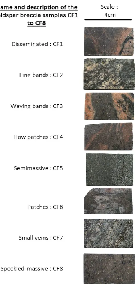
The samples used in this study come from LKAB’ mine in Malmberget and were classified earlier in eight classes as shown on figure 17 (Lund, in prep.). In order to classify and manage information, a database is built based on three following data structures described on figure 14.
Figure 14 : Data structures used to classify the samples
The collar structure is the raw information from the drill core. It includes the spatial coordinates and an identification code (ID). On the sample level, adjacent sections of the drill core of the same kind of rock are selected. The composite structure will classify different samples into groups that have similar geometallurgical properties. The composite table is presented in appendix B.
The samples received were already composites in limited amount, so that a selection was made in order to ensure that a sufficient and representative quantity of material was tested. The samples include 10 different classes based on the mineralogy of the gangue and textural properties and classified by (Lund 2013) as shown on Figure 15. The approach is to analyze the response in terms of physical properties,
Collar
structure
•Drillhole ID
•Spatial data (X,Y,Z,Dip 1,Dip 2)
Sample
structure
•Drillhole ID
•Range of the drill hole •Weight
Composite
structure
•Composite ID •Sample ID •Drillhole ID•Depth range slected in the drillhole •Weight
33
crushability, grindability and degree of liberation of the classes defined from CF1 to CF8 for feldspar-rich samples and CRC or CRF for amphibole-rich high grade ore samples from rock mechanics tests at a milimetric scale down to liberation analysis at a micrometric scale.
CRC and CRF are used as reference samples for liberation but are not included in the clustering process since they represent a different rock material with rather different modal composition and texture. The main purpose of having those classes is to provide information about how the grain size influences the liberation.
CF1 to CF8 are composites mostly from Fabian and some from Printzsköld ore bodies whereas CRC and CRF come from Hens.
Figure 15 : Samples classification system (Lund C. 2013), modified
Sample material was first used for mechanical tests, then underwent comminution and was split according to size fraction for both SEM analysis and XRF analysis as shown on Figure 16 .
34
35
36 b. Rock mechanics material and methods
i. Point load test (PLT)
The received material consisted of quarters of drill cores with a radius between 15 and 20 mm and a length between 10 mm and 200 mm. Unified dimensions of a 15 mm radius (L) and 30mm (D) length were chosen. Afterwards, each sample has been measured and weighted to obtain an estimated specific gravity for the rock material.
According to the D5731-08 standard ((ASTM) 2011), the following conditions should be respected: • 30 to 85 mm test diameter for irregular lumps, rock cores or blocks : verified with D=30 mm • At least 10 samples for core or block samples: verified initially, though some of them were
categorized as invalid.
• Controlled water content: verified since all the samples were stored in the same conditions. • 10 to 60s before failure : verified
• 0.3L<D<L as on Figure 9 : not verified, a D/L ratio of 2 was chosen due to the available material Given the limited availability of sample materials in terms of shape, those tests were conducted in conditions as similar as possible to these standards. In particular, a test is regarded as valid only if the fracture is continuous from the top contact point between the test machine and the sample to the bottom contact point as shown on Figure 18.
Figure 18 : PLT validity criterion adapted to non-standard samples
As a result of this validity requirement, some test results have been dropped out and are referred to as invalid in the data file. The number of tests varied according to the initial total mass of material, the behavior during the test, notably for CF6 which displayed some heterogeneity reflected directly by a high rate of invalid point load tests.
37
Table 1 : Sample material properties and number of valid mechanical tests per class Class Mean specific gravity [] Total mass [g] Valid PLT Valid CT
CF1 2.525 626 8 9 CF2 2.658 840 13 13 CF3 2.992 537 15 13 CF4 3.500 1585 12 12 CF5 2.717 626 10 11 CF6 3.561 1021 6 13 CF7 3.505 720 11 10 CF8 4.203 782 10 11 CRC 4.307 2339 13 15 CRF 4.659 1470 14 15
ii. Simple compressive test (CT)
Simple compressive tests were conducted in the mineral processing lab at LTU, with samples of same size and shape as for the point load test. To be as close as possible to an uniaxial test : the speed of charge was kept low to avoid as much as possible dynamic effects (time of load between 1 and 4 minutes), the samples had a D/L ratio of 2 to avoid instabilities or overestimation of the strength and the samples were stored in the same conditions (room temperature close to 20°C, relative humidity of 70%)(Charlier 2009).
c. Comminution material and method
In this work, the comminution test includes a first run in a jaw crusher with a 5 mm opening to produce sample material below 3.5 mm. The second step consists of a ball mill running for 20 minutes with 1L of water for 1.2 kg of solid material. The energy drawn by the mill was recorded and a sieving curve has been established for each class after each step. This work was done in the mineral processing laboratory at LTU.
The grinding step was used to study the behavior of different mineral textures during comminution and link it to liberation characteristics.
38
XRF analysis was used to compare and validate the results from the SEM but also to get modal analysis for all size fractions. The analysis in itself was carried on by LKAB at Malmberget and included Fe(II) for all samples in all the size fractions except CF65X, CRC5X and CRF5X for which the amount of sample was not sufficient for a proper Fe(II) measurement.
In this study, XRF was used to validate the results from the EDS acquired with the Merlin SEM. Given that XRF provides elemental analysis whereas INCA gives mineral grades, an operation of mass-balancing called Element to Mineral conversion (EMC) was applied as described in (Lund 2013).
The EMC was done in three rounds, the first one using a normal least squares method (LS) and the two next rounds using a non-negative least square (NNLS) method to solve the minimization problem described in section c. Regarding Fe (II), it has been assigned to magnetite, resulting in an overestimation of hematite when no measurement of Fe (II) was available. In table 2, mineral names are abbreviated according to this list:
• Magnetite : Mgt • Hematite : Hem • Ilmenite : Ilm • Albite : Ab • Apatite : Ap
• Tremolite : Tr (no distinction within the tremolite-actinolite solid-solution) • Orthoclase : Or
• Biotite : Bt • Quartz: Qtz
Table 2 : Settings for the element to mineral conversion Round Minerals Elements Method
1 M/Ab/46 M/Ap/504 P XRF Na XRF LS 2 M/Bt/1721 M/Tr/447 M/Or/3594 M/Qtz/53 K XRF Mg XRF Ca XRF Al XRF Si XRF NNLS 3 M/Hem/79 M/Mgt/80 M/Ilm/837 Fe XRF Fe II Ti XRF NNLS
Since it is difficult to make a difference between iron oxides on the SEM, all the iron oxides have been measured as magnetite which in fact covers magnetite but also hematite and possibly other iron oxides.
39
To account for this effect, all the iron oxides given by the element-to-mineral conversion have been summed up and then compared to the magnetite grade obtained by the SEM.
e. SEM liberation material and method
The liberation analysis was carried using a Merlin High-Resolution FEG-SEM available at LTU using the following detectors:
• InLens-backscattered electrons (BSE) detectors • Energy-dispersive spectrometry (EDS) detector The column itself is presented on figure 19.
Figure 19 : Merlin SEM column schematic (Zeiss 2011)
The liberation analysis involved a quantitative study of minerals with measurements by a SEM and processing by INCAMineral software (INCA 2011) . Based on the liberation data , the determination of the association index (AI) was done with HSC Geo (Lamberg 2011). The association index gives a criterion to categorize textural archetypes and is discussed in a later section.
40
Samples for liberation analysis consisted of cylindrical epoxy-resin mounts (prepared at Oulu University) coated with carbon (done at LTU). A first test was run with CF61 to compare the liberation results obtained by backscattered electrons (BSE) only and BSE-imaging with energy-dispersive spectrograph (EDS). A motivation for this was the time needed, given that BSE-only measurements are much faster than EDS. The two techniques show a clear difference both in terms of modal mineralogy and liberation of magnetite (EDS gave 80 % liberated magnetite whereas only BSE gave 60 %), these results are displayed in the appendix. As a result, all samples have been processed with EDS measurements to ensure the quality of the data.
The main measurement settings for the microscope were a magnification of 400x for fine grains samples and 200x for coarse grain in order to have enough particles within the sample. INCAMineral provides one file per sample, which includes modal composition for each particle, particles count, shape and area of each particle and statistics. The general process to produce these files is the following (OxfordInstruments 2012) :
• Subdivide the whole measurement area into smaller fields
• Acquire BSE image of the field and apply morphological operations to obtain separated particles. This step is important because some problems may arise from incorrectly de-agglomerated particles like two nearby particles to be counted as one
• Perform an EDS measurement on each grain to identify and quantify the mineral phases of the grain, based on either full-spectrum rules or simple ones (Lamberg 2013)
• Store all the measurements in the file for further processing
The minerals identified by rules were magnetite (Mgt), albite (Ab), orthoclase (Or), apatite (Ap), biotite (Bt) and tremolite (Tr). In this work, no distinction is made within the actinolite-tremolite solid-solution terms so the term tremolite is used to describe anything between actinolite and tremolite end-members. If the identification fails, it will be labeled as unknown or “others”. The fact that no distinction was made between different iron oxides and that Ilmenite was not included will result in the classification of all these iron-containing phases as magnetite.
The first step was to treat the particles files obtained by the SEM (and INCAMineral software) to obtain a file where all the particles and their properties are included for all size fractions for a given sample. After that, using a binning algorithm on the particles for each size fraction, useful graphs are constructed such as liberation curves per element for each size fraction, mineral composition of each size fraction and the mode of occurrence of magnetite which describes the amount binaries or ternaries of magnetite with gangue minerals with the Geo module of the HSC Chemistry software.
41
f. Liberation model by archetypes material and method
The use of archetypes to describe the liberation is the main hypothesis of this work. This has been done by processing the data from SEM and INCAMineral with HSC Geo 7.18 (Lamberg 2011).
A first technique is available to validate the archetype: iterative rebalance. In this process, we will use the liberation data of the first sample (archetype) but replace the modal composition by the one of another sample. The assumption is that grade by size will follow the trend observed in the archetype. By doing this, particles of the archetype will be rebalanced to match the modal composition of the second sample. The liberation key figures, degree of liberation and association index for magnetite, are calculated for the rebalanced product. This process is based on iterative formulas described by (Lamberg 2012) in equations (12) and (13).
For each mineral i in a given size fraction, the mineral grade in the sample for the current size fraction (M(i)fraction) is compared to the sum of the product of the mass proportion of particle in the current size fraction (p(j)fraction) multiplied by the mass proportion of mineral i in a particle (x(i)p). This sum is the mineral grade calculated from the liberation of the archetype.
𝑘
𝑖,𝑓𝑟𝑎𝑐𝑡𝑖𝑜𝑛=
∑𝑛 (𝑝(𝑗)𝑀(𝑖)𝑓𝑟𝑎𝑐𝑡𝑖𝑜𝑛𝑓𝑟𝑎𝑐𝑡𝑖𝑜𝑛𝑥(𝑖)𝑝)𝑗=1
(12) For each iterative step, the mass proportion of particle j in the current size fraction (pj,fraction) is then corrected with the correction factor ki,fraction
.
𝑝
𝑗,𝑓𝑟𝑎𝑐𝑡𝑖𝑜𝑛= 𝑝
𝑗,𝑓𝑟𝑎𝑐𝑡𝑖𝑜𝑛∑ (𝑥(𝑖)
𝐿𝑗=1 𝑗𝑘
𝑖,𝑓𝑟𝑎𝑐𝑡𝑖𝑜𝑛)
(13)
With this iterative process, the modal composition of a sample is used to generate a new particle population based on an archetype. This population will be compared to the measured population in terms of liberation and association index to verify the ability of the chosen archetype to describe the sample.
If the difference between the initial liberation key figures and the rebalanced is small, it means that, despite different modal compositions, the samples are texturally similar, i.e. the other sample shows similar liberation distribution when compensated against modal mineralogy. If the difference is high, the second sample represents another texture class and cannot be used as an archetype for the first sample.
42
In this case, the +53 µm size fraction (containing CF22, CF42, CF62, CRC2 and CRF2) was chosen since it had been completely analyzed and that each SEM measurement includes a sufficient number of particles.
A second tool to evaluate if a given sample class can be used as an archetype, is to use the Association Index (AI). It is defined for a target mineral (here, magnetite) and a given gangue mineral (i) as
𝐴𝐼(𝑖, 𝑡𝑎𝑟𝑔𝑒𝑡) =
𝑎𝑠𝑠𝑜𝑐𝑖𝑎𝑡𝑖𝑜𝑛(𝑖,𝑡𝑎𝑟𝑔𝑒𝑡)𝑔𝑟𝑎𝑑𝑒(𝑖)(14) The grade in mineral I is known by modal mineralogy and association (i,target) is obtained by summing the proportion of binaries “mineral i –target mineral” and ternaries “mineral i – mineral j – target”, divide it by (100-Liberated magnetite-association(others, magnetite) and multiply the whole by 100. An example is displayed on figure 20.
This value can be calculated for each mineral pair but here it was calculated only for each mineral associating with magnetite (i.e. magnetite-albite, magnetite-tremolite, magnetite-apatite, …). It is a non-dimensional measure of the affinity for magnetite to be associated with the gangue minerals as a binary or ternary with the target mineral. To calculate AI, only the modal composition and the mode of occurrence of magnetite (association) are needed.
For every gangue material we can evaluate the association of it with magnetite by summing the amount of binary and ternary associations of magnetite with this given gangue mineral and divide it by the total amount of the gangue mineral (when magnetite is excluded). This will give the mass of locked magnetite associated with that given gangue material. If we divide this quantity by the modal composition in that gangue mineral, normalized to exclude magnetite, we get a ratio of the weight of magnetite associated with that given gangue material and the grade of that gangue material.
43
Figure 20 : Simple example of association index (AI)
This means that
• If AI = 1, association of magnetite with the gangue mineral is expected by the gangue grade; i.e. AI indicates random texture and breakage for magnetite and gangue.
• If AI > 1, association of the magnetite with gangue mineral is preferential. This can be due to non-random, preferential texture or preferential breakage or both.
• If AI < 1 then magnetite association with the gangue mineral in particulate material is non-preferential. This may be due to texture or preferential breakage or both.
For each size fraction and for each gangue mineral an association index can be calculated. By its definition, if we assume an equal distribution of gangue minerals in all size fractions, AI should be independent of the size fraction. If some variation of AI across different size fractions is observed, that means that preferential breakage occurred for that gangue mineral.
Thus, the second step is to calculate an initial AI for each sample class and compare the values of AI for the main gangue minerals between different sample classes.
If for a given class, the degree of liberation and AI for gangue minerals does not change much when using an archetype, then that archetype is valid and can be used to describe that given class.
44
5. Results
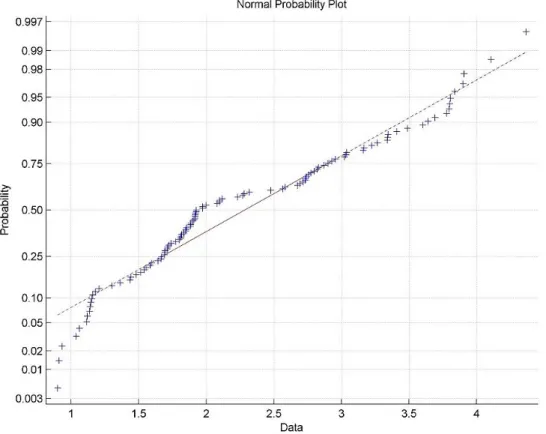
a. Rock mechanics analysis i. Point load test (PLT)
The results of the PLT for the whole population let appear a multimodal distribution on the normal probability plot as shown on Figure 21. Therefore, it makes sense to analyze the data per class, based on the mean of each class. Moreover, since the sample size in each class is small, a Student’s-t distribution is used instead of a normal distribution. As an effect of this hypothesis, the formula to evaluate the confidence interval (CI) for the mean is given by equation (15).
𝐶𝐼 = 𝑥
��� ± 𝑡
𝑛 𝛼2,𝑛−1
𝑆𝑛
√𝑛
(15)
Where xnis the sample’s mean, t the Student’s t value found in tables, Sn the standard deviation of the sample and n the size of the sample.
45
Figure 22 : Is(50) mean values and 95 % CI bars for CF1 to CF8
No continuous trend is seen for the Is(50) values despite an overall decrease from CF1 to CF8. This can be understood given the heterogeneity of the rock material: iron ore breccia composite samples. However, CF1 and CF2 have higher mean values whereas CF7 and CF8 form a lower-valued group. Caution is required for CF1, CF2 and CF6 given the large confidence interval resulting of a small sample size (CF6) or ore breccia natural heterogeneity.
The Point Load Test results for each class may be found in a graphical form the Appendix A and as a table in Appendix B.
ii. Simple compressive test (CT)
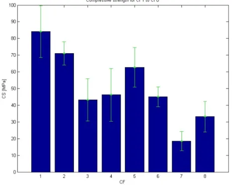
One of the expected results from the compressive test is a correlation with the Point Load Test with a linear correlation coefficient within the interval [15;50] as seen on equation (3). As shown on Figure 23, a good approximation (norm of residuals = 22.39) is given by equation 16
46
Figure 23 : Correlation between Is(50) and compressive strength
Given the correlation, the general trend of the mean compressive strength displayed on Figure 24 is the same as for Is(50). A difference lies in the fact that despite a similar decreasing trend from CF1 to CF8, the confidence intervals are much larger.