Using Bags of Visual and Textual Terms with
Extremely Randomized Trees:
Report of ImageCLEF 2010 Experiments
Rapha¨el Mar´ee, Olivier Stern, and Pierre Geurts
GIGA Bioinformatics
Avenue de l’Hopital 1, 4000 Li`ege Sart-Tilman University of Li`ege, Belgium
{raphael.maree,olivier.stern,pierre.geurts}@ulg.ac.be http://www.giga.ulg.ac.be
Abstract. In this paper we describe our experiments related to the ImageCLEF 2010 medical modality classification task using extremely randomized trees. Our best run combines bags of textual and visual features. It yields 90% recognition rate and ranks 6th among 45 runs (ranging from 94% downto 12%).
Keywords: extremely randomized trees, random subwindows, bag-of-features, image classification
1
Task description
We participated in the ImageCLEF 2010 task related to imaging modality clas-sification1
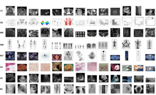
. A set of 2390 (in color or greylevels) training images were provided. These were extracted by the organizers of the challenge from articles published in scientific journals (Radiology and Radiographics) together with the text of the figure captions and the title of articles. Images have been classified by experts into the following 8 classes that are illustrated by Figure 1:
– CT: Computerized tomography (314 images)
– GX: Graphics, typically drawing and graphs, (355 images) – MR: Magnetic resonance imaging (299 images)
– NM: Nuclear Medicine (204 images)
– PET: Positron emission tomography including PET/CT (285 images) – PX: optical imaging including photographs, micrographs, gross pathology
etc (330 images)
– US: ultrasound including (color) Doppler (307 images) – XR: x-ray including x-ray angiography (296 images)
1
Fig. 1. Images for each of the 8 classes of the ImageCLEF 2010 imaging modality classification task (from articles published in Radiology and Radiographics).
The goal of the task is to build classification models able to recognize the imaging modality, using visual information only, textual information only, or both. Such models are expected to improve further content-based image retrieval. Participants submitted their predictions on a independent test set of 2620 images (for which modality classifications were not available) and classification results were later evaluated by organizers. A total of 45 runs were submitted by 7 research teams. In this paper, we report our results exploiting visual and textual information independently or combined using extremely randomized trees in a straightforward fashion.
2
Method
2.1 Generation of bags of textual terms
We adopted the bag of words model that is widely used in natural language processing and information retrieval. We processed the provided XML file using a Python script to build a dictionary of all unique term (words) from the training set of image captions and article titles. More precisely, the XML file is cleaned (by removing XML tags and unuseful characters, and lowering characters) and a dictionary is built which finally consists of 13553 unique terms. Each image was then described by 13553 features where each feature is simply the term frequency ie. the number of times a given term appears for that image (in its caption and title) normalized by the number of terms for that image (in its caption and title), so that each textual feature is comprised in the [0, 1] interval.
2.2 Generation of bags of visual terms
Despite many years of research in feature extraction, decribing image content is not a trivial task when facing a new image classification problem. We adopt here a generic approach that learns a global, bag of visual words, image rep-resentation by using dense random subwindows extraction [MGPW05,MGW07] and extremely randomized trees [GEW06,MNJ08,MGW09]. More precisely, from each training image, we extracted 2000 small subwindows (which sizes were ran-domized between 10% and 25% of image sizes) at random positions in images, we resized them to 16 × 16 patches and described them by 768 HSV raw values, as illustrated by Figure 2.
Fig. 2. Random subwindows extraction and description by raw pixel values.
We then built T = 10 extremely randomized trees using K = 28 random tests in each tree node and a minimum node sample size of 4000 (see Section 2.3 for algorithm details). Subwindow sizes and minimum node sample size were optimized on the training set by cross-validation. Other parameters were set to
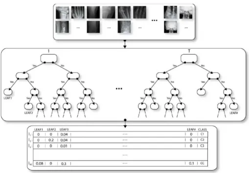
default values but further optimization might improve results. These parameter values yield 52660 terminal nodes in the ensemble of trees. Each terminal node (or leaf) of a tree is then used as visual feature (also known as “codebook” or “visual word”). By propagating image subwindows downto trees, each image is thus described by a global feature vector which dimensionality equals the number of terminal nodes in the ensemble of trees. For a given image, the value encoded for a given feature was equal to the visual term frequency, ie. the number of image subwindows that reach this terminal node divided by the total number of subwindows extracted in the image (so a leaf value is included in [0, 1], and the sum over all terminal nodes equals to 1 in a given tree for a given image), as illustrated by Figure 3.
Fig. 3. Training an ensemble of trees from random subwindows to build bags of visual terms.
2.3 Extremely Randomized Trees Classifier
Once features are built, they are concatenated and fed into a machine learn-ing algorithm to build a classifier. We used the extremely randomized trees algorithm [GEW06] that was successfully used in various application domains (e.g. [GdF+
im-age classification tasks where it was already combined with random subwindows extraction [MGPW05,MGW07].
Starting with the whole training set at the root node, the Extra-Trees algo-rithm builds an ensemble of decision trees according to the classical top-down decision tree induction procedure [BFOS84] that uses tests on input variables to progressively partitions the input space into hyperrectangular regions so as to yield regions where the output is constant. The two main differences between this algorithm and other tree-based ensemble methods are that it splits nodes by choosing both attributes and cut-points at random (rather than choosing the best cut-point that optimizes a score measure like in Tree Bagging [Bre96] or Random Forests [Bre01]) and that it uses the whole learning sample (rather than a bootstrap replica in Tree Bagging and Random Forests) to grow the trees.
In our case, we use extremely randomized trees to build visual features from images as already mentionned in previous section, but also as final classifier either on textual or visual features or both.
In the case of construction of visual features where subwindows are described by raw pixel values, a test associated to an internal node of a tree simply com-pares the value of a pixel (intensity of a grey level or of a certain color component) at a fixed location within a subwindow to a cut-point value. In the case of its use as final classifier, a internal test compares the value of a (textual or visual) feature to a cut-point value.
In order to filter irrelevant attributes, the filtering parameter K corresponds to the number of input features chosen at random at each node, where K can take all possible values from 1 to the number of variables describing the training objects (e.g. 768 when building visual features from HSV subwindows; 13553 when building trees on textual features only). For each of these K attributes, a numerical threshold is randomly choosen within the range of variations of that attribute in the subset of objects available in the the current tree node. The score of each binary test is then computed on the current training subset according to an information criterion (the score measure is defined in [Weh97] and corresponds to a measure of impurity), and the best test among the K tests is chosen to split the current node into two nodes. Objects that fulfill the choosen test are propagated to the left child node, and others to the right node, and the process is repeated recursively on both child nodes. The development of a node is stopped as soon as either all input variables or the output variable are constant in the local subset of the leaf (in which cases impurity can not be further reduced), or the number of objects in the leaf is smaller than a predefined value (the minimum node sample size, nmin). A number T of such trees are grown from the training sample.
3
Results
3.1 Textual features only
Using T = 10000 trees and K =√13453 = 116 random tests in each tree node, we obtain 85% recognition rate on the independent test set using textual features
only. This result is comparable with results we obtained by cross-validation on the training set (86%). Table 3.1 gives the first 50 textual terms used by the ensemble of trees and their relative importance for each class. Among the 13553 terms, the model is able to select very relevant ones to discriminate imaging modalities (e.g. the active molecule FDG for PET, the term photograph for PX, the scintigraphy test for NM, . . . ) but it does not filter out several artefacts neither rather neutral words (A, B, BB, BBB, IN, . . . ).
3.2 Visual features only
Using T = 10000 trees and K =√52660 = 230 random tests in each tree node of the final classifier, we obtained 75% recognition rate on the independant test set. This result is slightly better than results we obtained by cross-validation on the training set (71.75%).
3.3 Combination of textual and visual features
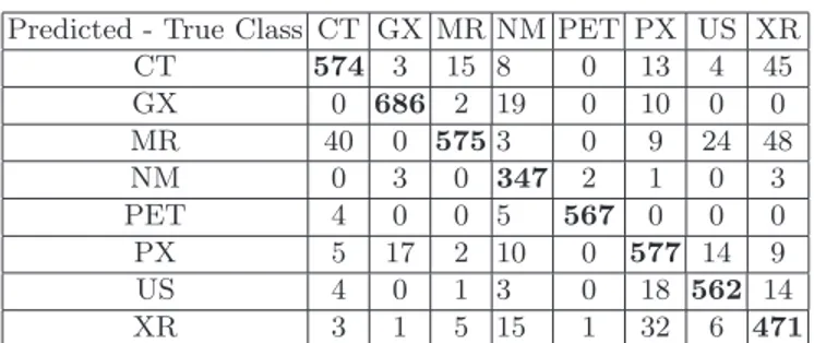
Building an ensemble of T = 10000 trees using both textual and visual features (ie. 62213 input features) raised results up to 90% recognition rate. This final result is comparable with results we obtained by cross-validation on the training set (90.377% recognition rate using both feature types, see the confusion matrix in Table 2). To reduce computing times and give less importance to visual fea-tures than textual feafea-tures, we introduced a new parameter, p, that indicates the proportion of visual features (randomly choosen) that each tree will use as input features. The value of K was fixed to its default value K =√13453 + p × 52660. The submitted result was obtained with p = 0.05 so that each tree was able to use 13553 textual features and 2633 (52660 × 0.05) visual features. This value yielded the best results by cross-validation on the training set.
Table 3 shows contribution of both feature types for each class. Visual fea-tures are the most useful for the GX (Graphics, typically drawing and graphs) imaging modality while textual features are the most useful for the PET imaging modality. Table 4 illustrates some test images and their classification confidences using individual feature types of a combination of them.
It has to be noted that we also experimented with LIBLINEAR2as final clas-sifier on both feature types but results were slightly inferior (86.42% recognition rate by cross-validation on the training set) to those obtained with extremely randomized trees.
3.4 Computing times
Our approach consists in rather simple operations, especially for the prediction phase. First, the training of 10 trees for the bag of visual terms construction takes about 20 hours when using about 4.6 million subwindows (2000 subwindows for each of the 2320 training images) on a single processor. This training phase is
2
Term Importance CT GX MR NM PET PX US XR US 100.00 1.77 0.64 1.47 0.35 0.44 0.54 17.32 1.49 CT 98.05 15.73 0.44 1.56 0.61 0.54 0.76 1.96 1.80 MR 65.64 1.22 0.52 10.74 0.41 0.56 0.48 1.05 1.06 PET 63.86 0.87 0.31 0.41 0.59 12.96 0.24 0.39 0.45 FDG 62.09 0.79 0.30 0.37 0.61 12.69 0.25 0.37 0.41 T-WEIGHTED 53.56 0.65 0.72 9.66 0.22 0.30 0.34 0.56 0.59 PHOTOGRAPH 52.03 0.64 0.68 0.42 0.17 0.14 8.67 0.44 0.76 SCAN 43.08 4.57 1.18 0.86 0.40 0.85 0.47 0.78 1.16 RADIOGRAPH 42.44 0.77 0.63 0.51 0.23 0.12 0.28 0.46 7.37 UPTAKE 36.59 0.65 0.24 0.36 3.11 4.47 0.29 0.36 0.47 GRAPH 35.56 0.27 6.15 0.28 0.09 0.08 0.21 0.32 0.35 IMAGE 32.86 0.49 1.32 2.42 0.30 0.19 0.69 1.51 0.90 STAIN 26.87 0.20 0.31 0.24 0.08 0.09 4.79 0.21 0.22 ORIGINAL 24.51 0.18 0.25 0.25 0.08 0.09 4.38 0.18 0.20 FOR 23.46 0.43 3.09 0.32 0.19 0.20 0.23 0.33 0.50 MAGNIFICATION 22.58 0.18 0.31 0.23 0.08 0.09 3.91 0.19 0.17 -YEAR-OLD 22.44 0.97 1.88 0.47 0.26 0.29 0.41 0.29 0.65 PHOTOMICROGRAPH 22.34 0.18 0.21 0.19 0.07 0.07 4.01 0.20 0.17 SCINTIGRAPHY 19.38 0.15 0.12 0.10 5.34 0.20 0.08 0.11 0.16 SCINTIGRAM 19.34 0.14 0.12 0.08 5.42 0.14 0.08 0.12 0.17 ARROW 18.96 0.82 1.76 0.33 0.21 0.27 0.23 0.31 0.45 PET-CT 18.94 0.23 0.09 0.09 0.15 3.96 0.08 0.10 0.11 IMAGES 16.81 0.29 0.54 1.38 0.22 0.47 0.43 0.33 0.41 ACTIVITY 16.00 0.23 0.13 0.15 2.65 1.03 0.09 0.16 0.24 FONT 15.77 0.16 0.16 0.16 0.09 0.10 2.62 0.16 0.19 SPECIMEN 14.96 0.23 0.19 0.18 0.07 0.07 2.28 0.17 0.27 AXIAL 14.80 0.67 0.35 0.96 0.18 0.54 0.20 0.22 0.48 PETCT 14.10 0.15 0.08 0.09 0.06 2.95 0.05 0.09 0.09 A 13.93 0.40 1.02 0.29 0.21 0.12 0.42 0.33 0.48 ARROWS 13.87 0.36 1.11 0.34 0.16 0.11 0.23 0.50 0.42 RADIONUCLIDE 13.58 0.12 0.09 0.07 3.69 0.12 0.09 0.06 0.13 HYPOECHOIC 13.54 0.19 0.10 0.19 0.04 0.05 0.11 2.46 0.11 AB 13.01 0.19 0.21 0.26 0.38 0.04 0.81 0.70 0.58 IMAGING 12.95 0.36 0.20 1.12 0.44 0.15 0.22 0.31 0.42 FUSED 12.65 0.16 0.07 0.07 0.09 2.62 0.05 0.08 0.07 LONGITUDINAL 12.40 0.23 0.09 0.09 0.06 0.05 0.08 2.22 0.16 DOPPLER 12.14 0.14 0.07 0.15 0.04 0.05 0.07 2.27 0.12 HEMATOXYLIN-EOSIN 11.79 0.09 0.13 0.10 0.04 0.05 2.09 0.09 0.09 SHOWS 11.58 0.37 0.54 0.32 0.22 0.13 0.40 0.39 0.40 OBTAINED 11.16 0.53 0.62 0.23 0.27 0.15 0.23 0.26 0.38 TRANSVERSE 11.00 0.52 0.41 0.22 0.13 0.10 0.15 0.71 0.38 IN 10.93 0.36 0.28 0.26 0.25 0.55 0.33 0.30 0.36 TC-M 10.68 0.09 0.06 0.05 2.97 0.06 0.04 0.09 0.09 SAGITTAL 10.63 0.20 0.26 1.05 0.08 0.10 0.16 0.46 0.24 CORONAL 10.46 0.22 0.30 0.44 0.15 0.95 0.12 0.14 0.24 BAB 10.39 0.31 0.64 0.29 0.25 0.20 0.23 0.24 0.32 B 10.23 0.27 0.75 0.22 0.29 0.17 0.17 0.23 0.34 BBB 10.00 0.31 0.60 0.26 0.21 0.18 0.26 0.24 0.31 BB 9.89 0.31 0.25 0.18 0.44 0.07 0.37 0.40 0.45 SPECT 9.81 0.07 0.03 0.07 2.73 0.10 0.04 0.06 0.08 Table 1. The top 50 textual terms according to their importance given by 10000 extremely randomized trees.
Predicted - True Class CT GX MR NM PET PX US XR CT 574 3 15 8 0 13 4 45 GX 0 686 2 19 0 10 0 0 MR 40 0 575 3 0 9 24 48 NM 0 3 0 347 2 1 0 3 PET 4 0 0 5 567 0 0 0 PX 5 17 2 10 0 577 14 9 US 4 0 1 3 0 18 562 14 XR 3 1 5 15 1 32 6 471
Table 2. Confusion matrix obtained by cross-validation on the training set using both feature types (90.377% recognition rate).
Feature type CT GX MR NM PET PX US XR Textual 0.07 0.02 0.08 0.06 0.09 0.07 0.07 0.06 Visual 0.06 0.12 0.05 0.03 0.03 0.07 0.06 0.06
Table 3. Class importance of feature types given by 10000 extremely randomized trees on the training set.
only performed once using all training images. Building the 10000 trees of the final classifier requires about 4 hours. Once trees have been built, the bag of visual terms of one test image is constructed on average in 0.83s (0.65s for the extraction and resizing of 2000 subwindows, 0.18s for their propagation in the ensemble of 10 trees). Computing the bag of textual term frequencies for test images requires 0.03s per image on average. Propagating an image (described by both textual and visual features) into the final classifier requires 0.01s per image. In total, a new image could then be described and classified roughly in less than 1s using both feature types on a single computer.
4
Conclusions
We obtained 90% recognition rate on the ImageCLEF 2010 modality classifica-tion task using a rather straightfoward and fast approach that combine textual and visual features. Optimization of parameters and other combination mecha-nisms might further improve results.
Acknowledgments. RM is supported by the GIGA (University of Li`ege) with the help of the Walloon Region and the European Regional Development Fund. PG is Research Associate of the F.R.S.-FNRS. This paper presents research results of the Belgian Network BIOMAGNET (Bioinformatics and Modeling: from Genomes to Networks), funded by the Interuniversity Attraction Poles Programme, initiated by the Belgian State, Science Policy Office. This work is supported by the European Network of Excellence, PASCAL2. The scientific responsibility rests with the authors.
Image ID True Class Textual Visual Both 32316 PX PX (0.81) XR (0.43) XR (0.47) 128482 MR GX (0.41) MR (0.38) MR (0.50) 36398 PX PX (0.80) CT (0.26) PX (0.32) 223797 GX XR (0.42) GX (0.98) GX (0.86) 63382 XR PX (0.29) PET (0.36) XR (0.45)
References
[BFOS84] L. Breiman, J.H. Friedman, R.A. Olsen, and C.J. Stone. Classification and Regression Trees. Wadsworth International (California), 1984. [Bre96] L. Breiman. Bagging predictors. Machine Learning, 24(2):123–140, 1996. [Bre01] L. Breiman. Random forests. Machine learning, 45(1):5–32, 2001. [GdF+05] Pierre Geurts, Dominique deSeny, Marianne Fillet, Marie-Alice Meuwis,
Michel Malaise, Marie-Paule Merville, and Louis Wehenkel. Proteomic mass spectra classification using decision tree based ensemble methods. Bioinformatics, 21(14):3138–3145, 2005.
[GEW06] P. Geurts, D. Ernst, and L. Wehenkel. Extremely randomized trees. Ma-chine Learning, 36(1):3–42, 2006.
[HTIWG10] Van Anh Huynh-Thu, Alexandre Irrthum, Louis Wehenkel, and Pierre Geurts. Inferring regulatory networks from expression data using tree-based methods. To appear in PLoS ONE (DREAM4 collection), 2010. [MGPW05] R. Mar´ee, P. Geurts, J. Piater, and L. Wehenkel. Random subwindows for
robust image classification. In Proc. IEEE CVPR, volume 1, pages 34–40. IEEE, 2005.
[MGW07] Rapha¨el Mar´ee, Pierre Geurts, and Louis Wehenkel. Random subwin-dows and extremely randomized trees for image classification in cell biol-ogy. BMC Cell Biology supplement on Workshop of Multiscale Biological Imaging, Data Mining and Informatics, 8(S1), July 2007.
[MGW09] Rapha¨el Mar´ee, Pierre Geurts, and Louis Wehenkel. Content-based image retrieval by indexing random subwindows with randomized trees. IPSJ Transactions on Computer Vision and Applications, 1(1):46–57, jan 2009. [MNJ08] Frank Moosmann, Eric Nowak, and Frederic Jurie. Randomized clustering forests for image classification. IEEE Transactions on PAMI, 30(9):1632– 1646, 2008.
[Weh97] L. Wehenkel. Automatic Learning Techniques in Power Systems. Kluwer Academic Publishers, Boston, November 1997.