Block Sparsity and Weight Initialization in
Neural Network Pruning
by
Arlene Elizabeth Siswanto
S.B., Massachusetts Institute of Technology (2020)
Submitted to the Department of Electrical Engineering and Computer Science in partial fulfillment of the requirements for the degree of
Master of Engineering in Electrical Engineering and Computer Science at the
MASSACHUSETTS INSTITUTE OF TECHNOLOGY February 2021
© Massachusetts Institute of Technology 2021. All rights reserved.
Author . . . .
Department of Electrical Engineering and Computer Science
January 15, 2021
Certified by . . . .
Michael Carbin
Assistant Professor
Thesis Supervisor
Accepted by . . . .
Katrina LaCurts
Chair, Master of Engineering Thesis Committee
Block Sparsity and Weight Initialization in Neural
Network Pruning
by
Arlene Elizabeth Siswanto
Submitted to the Department of Electrical Engineering and Computer Science on January 15, 2021, in partial fulfillment of the
requirements for the degree of
Master of Engineering in Electrical Engineering and Computer Science
Abstract
Block sparsity imposes structural constraints on the weight patterns of sparse neural networks. The structure of sparsity has been shown to affect efficiency of sparse com-putation in the libraries, kernels, and hardware commonly used in machine learning. Much work in the pruning literature has focused on the unstructured pruning of indi-vidual weights, which has been shown to reduce the memory footprint of a network, but cannot achieve the computational speedups that have become increasingly cov-eted as neural networks become deeper and more complex. On the opposite end of granularity, neuron pruning and channel pruning are unable to reach the same level of sparsity as unstructured pruning without compromising accuracy. Block-sparse pruning is a middle ground between these two extremes, with the potential for prun-ing to greater sparsities while still beprun-ing amenable for acceleration. Our fine-tunprun-ing experiments demonstrate that block-sparse pruning offers a tradeoff between granu-larity and accuracy; increasing block size results in a gradual decrease in accuracy. Our weight rewinding experiments show that increasing block size decreases the max-imum sparsity obtainable when pruning a network early in training. Finally, we make the surprising observation that randomly reinitializing the pruned network structure results in the same accuracy regardless of block size.
Thesis Supervisor: Michael Carbin Title: Assistant Professor
Acknowledgments
First and foremost, I would like to thank my thesis advisor, Professor Michael Carbin, for the opportunity to research with his group during both my undergraduate and graduate studies at MIT. His feedback and advice helped shape the direction of this thesis. The lab offered valuable insight into related topics of study as well as new ideas and perspectives during team discussions.
I would also like to express deep gratitude to Jonathan Frankle, who guided this work immensely and went above and beyond to make sure I had all the support and resources needed for the best possible experience. He has been my mentor in navi-gating the chaotic terrain of machine learning research, suggesting creative directions to explore and helping me ask the right questions. During both our in-person discus-sions and our pandemic-necessitated online chats, Jonathan has always been there to answer any and all questions, offer insight into his research experiences, and share advice and life musings. He has been beyond helpful in providing nuanced feedback about my work, allowing me to grow as a researcher. In addition, his work on the lot-tery ticket hypothesis and related topics laid the foundation for many of the questions investigated in this paper.
Next, I am thankful for the friends and memories I made during my time at MIT. The past few years have been exciting, formative, and full of experiences that have pushed me to grow as a person and to explore ideas and interests that I may not have otherwise considered. I am grateful for the friends that I was able to experience the high highs and low lows of the Institute with along the way.
Last but not least, I am grateful for my parents and sister, who have always encouraged me to do my best. I am thankful to have been raised in a supportive environment that allowed me to grow as a person. Without the freedom to explore ideas that interest me but also enough support to keep me directed, I would not have been able to be where I am today.
Contents
1 Introduction 15
2 Background and Related Work 17
2.1 Existing Pruning Literature . . . 17
2.1.1 Early Work . . . 18
2.1.2 Foundational Work . . . 19
2.1.3 Structured Pruning . . . 20
2.1.4 Neuron Pruning and Channel Pruning . . . 22
2.1.5 Block-Sparse Pruning . . . 22
2.1.6 Sparsity Acceleration . . . 24
2.1.7 Lottery Ticket Hypothesis . . . 25
2.2 Alternative Compression Techniques . . . 26
2.2.1 Distillation . . . 26
2.2.2 Quantization . . . 26
2.2.3 Low Rank Matrix Factorization . . . 27
3 Motivation and Contributions 29 3.1 Contributions . . . 30
3.1.1 Block-Sparse Accuracy and Lottery Tickets . . . 31
3.1.2 Random Reinitialization . . . 31
4 Pruning Terminology 33 4.1 Definitions . . . 33
4.2 Structure and Granularity . . . 33
4.3 Number of Runs . . . 35
4.4 Scoring . . . 35
4.5 Fine-Tuning and Weight Rewinding . . . 36
4.6 Evaluation . . . 36
5 Block Sparsity in Neural Networks 37 5.1 Methodology . . . 38
5.1.1 Selection of Benchmarks . . . 38
5.1.2 Pruning Specifications . . . 39
5.1.3 Block-Sparse Shapes . . . 39
5.2 Block Sparsity Implementation . . . 41
5.3 Results . . . 43
5.3.1 Experiments . . . 45
5.3.2 Long Strips vs. Square Blocks . . . 51
5.3.3 Intrakernel vs. Kernel-Level Blocks . . . 51
5.4 Discussion . . . 53
6 Block Sparsity and Reinitialization 55 6.1 Methodology . . . 56
6.2 Results . . . 56
6.2.1 Experiments . . . 57
6.3 Discussion . . . 65
7 Conclusion and Future Work 67 7.1 Concluding Remarks . . . 67
List of Figures
2-1 The left depicts a fully connected deep neural network: each neuron has weights connecting itself to every neuron in the next layer. The center and right are resulting networks after pruning. In weight prun-ing, individual weights are removed with no particular structure. In neuron pruning, a highly structured form of pruning, entire neurons have been removed. Neuron pruning effectively removes all the in-bound and outin-bound weights of a given neuron. Pruned weights are essentially set to zero in storage. . . 18 2-2 Number of publications per year containing the term “network
prun-ing.” The concept of neural network pruning has existed roughly since the 1990s, and has gained considerable traction since the introduction of deep networks such as AlexNet (2012), VGG (2014), and residual networks (2015) [31]. . . 19 2-3 Three-step pruning pipeline described by Han et al. (2015). Train
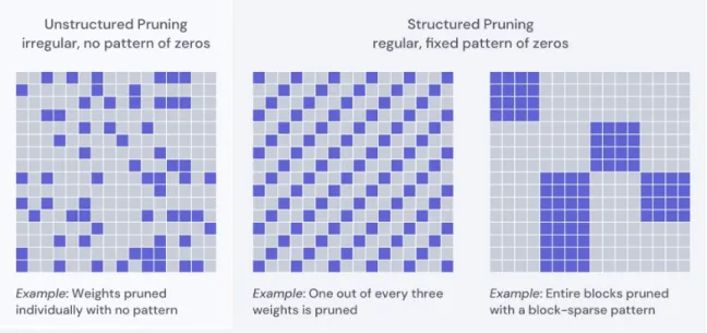
net-work to completion, remove the least important weights, then continue training the remaining sparse network to fine-tune. . . 20 2-4 Examples of unstructured and structured pruning. Unstructured
prun-ing is the scattered, unpatterned prunprun-ing of individual weights. Struc-tured pruning captures a range of techniques involving fixed rules and patterns, including block-sparse pruning. . . 21
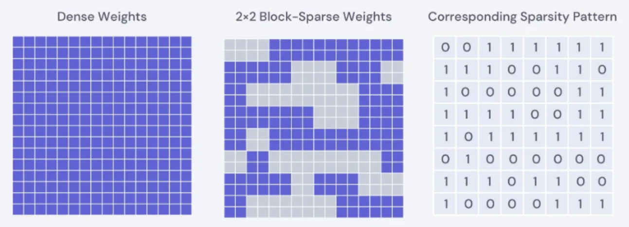
2-5 Representation of sparsity pattern for block-sparse weights. The left depicts weights of an unpruned fully connected layer. The center is an example of how these weights may look after pruned in a 2×2 block-sparse manner. The right displays a representation of this sparsity pattern. . . 23 5-1 Benchmark datasets used in image classification. MNIST contains
60,000 black-and-white handwritten digits. CIFAR-10 is a collection of 60,000 images spanning 10 categories. . . 39 5-2 Example of block-sparse pruning in fully connected layers. The gray
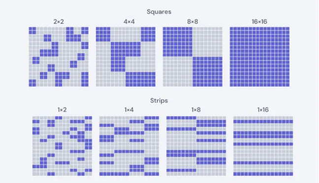
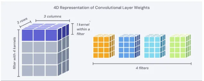
blocks have been pruned, while the blue blocks remain unpruned. We run experiments on power-of-two squares and long power-of-two strips. The bottom-right layer contains pruned strips, effectively the equiva-lent of neuron pruning. . . 40 5-3 Convolutional kernel sliding over an image. . . 41 5-4 4D representation of convolutional layer weights. Each kernel is made
of columns and rows. A filter is made of several kernels. There are several filters within a convolutional layer. . . 42 5-5 Effect of varying block granularity on accuracy for fully connected
LeNet trained on MNIST benchmark. Left: Networks with fine-tuning. Right: Networks with weight rewinding (lottery ticket). Blocks are long strips with a of-two side length (top) or squares with power-of-two side lengths (bottom). . . 46 5-6 Effect of varying block granularity on accuracy for ResNet-20 trained
on CIFAR-10 benchmark. Left: Networks with fine-tuning. Right: Networks with weight rewinding (lottery ticket). Blocks are composed of 1×3, 3×1, 3×3 blocks within a single kernel (top) or 1×1 squares power-of-2 kernels at a time (bottom). . . 48
5-7 Comparison of block shapes in fully connected layers, for fully con-nected LeNet trained on MNIST benchmark. Long strips and square blocks containing equal numbers of weights are compared. Left: Net-works with fine-tuning. Right: NetNet-works with rewinding (lottery ticket). 50 5-8 Compares varying intrakernel block shapes to varying block kernel
depth. Equal numbers of weights are compared. Left: Networks with fine-tuning. Right: Networks with rewinding (lottery ticket). . . 52 6-1 Pruning with random reinitialization for fully connected LeNet trained
on MNIST benchmark using various block granularities (part 1/3). Left: Comparison with fine-tuning. Right: Comparison with weight rewinding (lottery ticket). . . 58 6-2 Pruning with random reinitialization for fully connected LeNet trained
on MNIST benchmark using various block granularities (part 2/3). Left: Comparison with fine-tuning. Right: Comparison with weight rewinding (lottery ticket). . . 59 6-3 Pruning with random reinitialization for fully connected LeNet trained
on MNIST benchmark using various block granularities (part 3/3). Left: Comparison with fine-tuning. Right: Comparison with weight rewinding (lottery ticket). . . 60 6-4 Pruning with random reinitialization for ResNet-20 trained on
CIFAR-10 benchmark using various block granularities (part 1/2). Left: Com-parison with fine-tuning. Right: ComCom-parison with weight rewinding (lottery ticket). . . 62 6-5 Pruning with random reinitialization for ResNet-20 trained on
CIFAR-10 benchmark using various block granularities (part 2/2). Left: Com-parison with fine-tuning. Right: ComCom-parison with weight rewinding (lottery ticket). . . 63
6-6 Random reinitialization across many block shapes and sizes for ResNet-20 trained on CIFAR-10 benchmark using various block granularities. Left: All reinitializations with fine-tuning. Right: All reinitializations with weight rewinding (lottery ticket). . . 64
List of Tables
4.1 Possible choices while pruning. . . 34 5.1 Percent of weights remaining at the maximum sparsity attainable while
maintaining accuracy of the full network. We prune with various block shapes on fully connected LeNet trained on MNIST benchmark. . . . 45 5.2 Percent of weights remaining at the maximum sparsity attainable by
pruning with various block shapes for ResNet-20 trained on CIFAR-10 benchmark. . . 49 6.1 Difference in accuracy between standard and random reinitialization
with 6.9% of weights remaining when pruning with various block shapes for ResNet-20 trained on CIFAR-10 benchmark. . . 61
Chapter 1
Introduction
Deep neural networks have achieved remarkable success in solving complex tasks over large datasets. These models have become increasingly well-integrated into standard use, from smart devices to industrial production. Such widespread use has expedited the demand for models that are both computationally efficient and memory efficient. Pruning, which involves reducing the size of a neural network by removing parameters, is a well-studied compression technique for accelerating computation and reducing memory requirements. The large, dense matrices that constitute deep neural network architectures can be made sparse with little to no loss in model accuracy via pruning. Ideally, the sparse matrices that result from dramatically reducing the number of parameters in a model would allow for networks that feasibly consume fewer re-sources. In practice, however, these efficiencies may not be realized. Many existing pruning methods create unstructured random connectivity between weights in adja-cent layers. This lack of structure leads to irregular memory access that can hinder acceleration on hardware [38]. While in some instances, contemporary methods for executing unstructured sparse computations can improve performance, for other in-stances performance does not improve or in fact is reduced [8].
Structured pruning techniques allow us to take advantage of the fundamental efficiencies of sparse matrix computation and specialized hardware. On the extreme end, pruning entire neurons or channels means all inbound or outbound connections are no longer stored for that neuron or channel. Though this seems favorable, neuron
pruning has been shown to lead to notable drops in accuracy at lower sparsities than unstructured pruning [29]. Block-sparse pruning is a middle ground between unstructured weight pruning and this highly structured neuron and channel pruning. Block sparsity imposes structural constraints to pruning by removing entire blocks of neighboring weights at once. This remains an ongoing topic of research and its potential has not yet been comprehensively studied and documented. The goal of this work is to focus and expand the literature surrounding block sparsity.
The overarching question is as follows: given computational and memory con-straints, how can we arrive at the most accurate model? After discussing the ongoing literature in block-sparse pruning, we apply various granularities of block-sparse prun-ing to benchmark neural networks and compare accuracies with unstructured weight pruning. We consider two settings for our experiments. In the first, we fine-tune the previously learned weights in the network with the goal of understanding how much we can reduce costs at inference time. Our conclusion is that we must always make a tradeoff between accuracy and efficiency, as accuracy decreases when block size increases. In the second, we rewind weights to values found early in training from the previous pruning run in a way similar to that described in the lottery ticket hypothesis [9], with the goal of understanding the opportunity of reducing the cost of training. From this experiment, we find that we cannot train to full accuracy at the same sparsities as unstructured pruning while imposing block structure.
We also consider the role of learned weights in maintaining accuracy of the full net-work in block sparse pruning. We do this by comparing our results to their randomly reinitialized counterparts. Our surprising, yet notable, observation is that random reinitialization appears to obtain the same accuracy across block shapes and sizes. This leads us to believe that randomly reinitialized weights perform as well as learned weights not because of the representational ability of the resulting sparse network as suggested by Liu et al. [28], but instead because the imposed structural constraints of neuron and channel pruning hinder the accuracy of the sparse network to such a large extent.
Chapter 2
Background and Related Work
Neural networks contain a collection of nodes, or neurons, connected in a way vaguely inspired by neurons in the biological brain. The connections between biological neu-rons gradually and completely decay between birth and the mid-20s, in a process known as synaptic pruning [36]. In an analogous way, neural network pruning in-volves reducing the size of a network by removing weight parameters. Networks are generally believed to be overparameterized in practice, making it possible for redun-dant parameters to be removed without hurting accuracy up to a certain point. Given the same budget of parameters, sparsity enables the training of wider and deeper net-works, which are shown to have accuracies greater than smaller dense networks [41]. Pruning can be viewed as a tradeoff between model quality and model size, with the goal of maximizing model size reductions while minimizing loss in accuracy.
2.1
Existing Pruning Literature
Pruning has achieved wide appeal as a result of increasingly complex networks and the availability of unprecedented quantities of data. Figure 2-2 demonstrates the growth in pruning research since a notable study in 1990. One significant milestone was the three-step pruning pipeline introduced by Han et al. in 2015, discussed in Section 2.1.2. This method was able to reduce the number of weights in state-of-the-art networks of the time, such as AlexNet (2012) and VGG-16 (2014), by 9× and
Figure 2-1: The left depicts a fully connected deep neural network: each neuron has weights connecting itself to every neuron in the next layer. The center and right are resulting networks after pruning. In weight pruning, individual weights are removed with no particular structure. In neuron pruning, a highly structured form of pruning, entire neurons have been removed. Neuron pruning effectively removes all the inbound and outbound weights of a given neuron. Pruned weights are essentially set to zero in storage.
13× with no loss in accuracy – a success that accelerated further research on the topic. Variants of structured pruning, including the pruning of neurons, channels, and blocks, have since been studied.
2.1.1
Early Work
LeCun et al.’s 1990 paper on Optimal Brain Damage (OBD) [26] is among the earliest applications of pruning to neural networks. The work removed unimportant weights from a network, citing better generalization and improved speed of learning as bene-fits. The procedure for doing so involved using second-derivative information to make tradeoffs between network complexity and error, achieving a weight reduction of 4× on a state-of-the-art network of the time. Optimal Brain Surgeon (OBS) by Hassibi and Stork (1993) furthered this work by involving a recursion relation for calculating the inverse Hessian matrix from the training data, allowing for further reduction in weights [17].
Until recently, many pruning methods have required similarly complex tions. Analyzing these values for individual parameters quickly becomes
computa-Figure 2-2: Number of publications per year containing the term “network pruning.” The concept of neural network pruning has existed roughly since the 1990s, and has gained considerable traction since the introduction of deep networks such as AlexNet (2012), VGG (2014), and residual networks (2015) [31].
tionally intensive for large networks. More recent work has used simpler heuristics, such as the magnitude of a weight, to determine importance [39].
2.1.2
Foundational Work
Han et al. described a method for pruning redundant connections, aimed at reducing storage and computation needs of convolutional neural networks [16]. This method (shown in Figure 2-3), follows three steps:
1. Train the network to learn “important” connections. Han et al. used the magnitude of an individual weight as the importance metric.
2. Prune the least important connections. In the original paper, individual weights with magnitudes below a certain threshold would be removed. Other studies commonly remove a fixed percentage of remaining weights.
3. Fine-tune the network. This is done by continuing to train the network’s remaining unpruned connections.
Figure 2-3: Three-step pruning pipeline described by Han et al. (2015). Train net-work to completion, remove the least important weights, then continue training the remaining sparse network to fine-tune.
This procedure achieved a parameter reduction of 9× on AlexNet on the ImageNet dataset and a 13× on VGG-16. This success catalyzed further studies in recent years, and the method serves as a foundation for many pruning strategies today.
A method for deep compression by Han et al. in 2016 was a further extension of this work [15]. The paper combined pruning, trained quantization, and Huffman coding to reduce the storage requirement of the a neural network by 35× and 49× without affecting accuracy, a significant feat. Quantization reduces the number of bits representing weights. Huffman coding is an optimal prefix code used for lossless data compression, where more common symbols are represented with fewer bits. Such techniques that work alongside or in replacement of pruning can be found in Section 2.2.
2.1.3
Structured Pruning
Pruning can be described as unstructured or structured. In unstructured pruning, individual weights are pruned with no set pattern. This provides the highest amount of flexibility when selecting which weights within a network to remove. This also has the finest granularity of the pruning techniques. Previously discussed work by LeCun et al. (1990), Hassibi and Stork (1993), and Han et al. (2015) are focused on unstructured pruning [28].
Figure 2-4: Examples of unstructured and structured pruning. Unstructured pruning is the scattered, unpatterned pruning of individual weights. Structured pruning cap-tures a range of techniques involving fixed rules and patterns, including block-sparse pruning.
Structured pruning captures any technique that involves a fixed pattern of weight removal; for example those involving a rule (e.g. each block has a specific number of nonzero weights [40] [31]) or pattern (e.g. arbitrarily pruning one out of every three weights; Figure 2-4). These methods can range from coarse-grained to fine-grained. On the highly structured, coarse-grained end, neuron pruning and channel pruning remove entire neurons and convolutional filters from a network.
Imposing structure inherently removes a range of potential pruning options that a network has to maximize accuracy. In general, increasing structure tends to have a neutral or deleterious effect on accuracy. This has been corroborated empirically – removing entire neurons via neuron pruning has been shown to dramatically reduce attainable accuracy when compared to unstructured pruning [2], and removing entire filters also cannot match the accuracy of unstructured pruning [27]. Despite these deficiencies, structured pruning remains a worthwhile topic of exploration due to its potential for computational acceleration and memory usage reduction, discussed further in Sections 2.1.5 and 2.1.6.
2.1.4
Neuron Pruning and Channel Pruning
On the highly structured end, we have neuron pruning and channel pruning. In fully connected layers, entire neurons are removed from a layer. In convolutional layers, entire channels are removed from a layer by removing entire filters.
Various studies have shown that removing whole neurons or filters via regular-ization can achieve similar accuracy to removing individual weights up to 60-80% sparsity [2] [39] [27]. However, beyond this sparsity, it is unable to match the accu-racy of unstructured pruning, which can reach up to 95% sparsity without affecting accuracy. Thus far, it has been observed that at these greater sparsities, model quality cannot be preserved at coarser granularities.
In several ways, neuron pruning and channel pruning seem to behave differently from unstructured pruning. In unstructured pruning, it is common practice to pre-serve the learned weights from one run of pruning and to use these values at the beginning of the next. Liu et al. challenge this by randomly reinitializing weights at the beginning of a pruning run [28]. In neuron and channel pruned networks, they found that model quality remains the same using random reinitialization, suggesting the learned weights themselves do not matter. Another unstructured pruning obser-vation is that setting weights to values from early in training yields similar results as setting them to these learned weights. Liu et al. demonstrate that, in neuron and channel pruned networks, randomly reinitializing weights performs the same, which was not true for unstructured pruning. At what level of structuredness do these dis-crepancies between unstructured and highly structured pruning appear? Our work is concerned with understanding these discrepancies.
2.1.5
Block-Sparse Pruning
We explore block-sparse pruning as a middle ground between unstructured and highly structured pruning. In this form of pruning, entire contiguous neighborhoods of weights are removed at a time, as shown in Figure 2-5. Because block sparsity cap-tures a wide range of granularities between the two, understanding how it impacts
Figure 2-5: Representation of sparsity pattern for block-sparse weights. The left depicts weights of an unpruned fully connected layer. The center is an example of how these weights may look after pruned in a 2×2 block-sparse manner. The right displays a representation of this sparsity pattern.
model quality allows us to not only determine the block shapes and sizes at which preserving the weights from training matters, but also consider how to take advantage of efficiencies from increased structure.
Previous work has studied block-sparse pruning to various capacities. Mao et al. provide insights about how accuracy when pruning individual weights, rows or columns within a convolutional kernel, and entire kernels (the paper does not ex-plicitly describe its contributions using the term “block sparsity”) [29]. At sparsities of 60-75%, the three granularities maintain roughly the same accuracy, with un-structured pruning performing best by a small margin. The work demonstrates that coarse-grained sparsity saves about 2× of the total output memory references when compared to unstructured pruning accuracy at the same density; 3× when compared to the original dense implementation. In addition, on AlexNet, they found a small improvement (from 25.4% to 24.1%) in the number of floating point operations per second (FLOPs) which is commonly used as a measure of efficiency in deep neural networks. This work is closely related to our work, though our studies draw conclu-sions from a wider range of block sizes and shapes, and consider the problem in two additional contexts: the lottery ticket hypothesis and random reinitialization.
reg-ulation [29] [30] [27]], group regreg-ulation [38], and particle filtering [3]. Examples of networks it has been applied to include CNNs [29] [38] [3], RNNs [30], and Trans-formers [6]. Other work has focused on clever methods to maximize structure while block-sparse pruning [37]. Directions of work towards accelerating block-sparse com-putation is discussed in the next session.
2.1.6
Sparsity Acceleration
Maximizing advantages of structured matrix computation is an area of ongoing re-search. Structured matrices provide rules or patterns that unstructured matrices do not, and as a result, values are stored in memory in a more predictable fashion. Ac-cessing values stored in the main memory of a GPU core takes an order of magnitude longer than floating point calculations; therefore, accessing a larger amount of val-ues at the same time and performing many computations in parallel is essential for efficient compute. A CPU executes more efficiently with sequential, contiguous mem-ory access patterns, which corresponds to contiguous layouts of numbers in memmem-ory. Block-sparse matrices with large-enough blocks can produce these large contiguous accesses [24]. Specifically designed libraries, optimized kernels, and specialized hard-ware can all be used towards computational efficiency improvements and memory footprint reductions.
On the most user-directed level, open source libraries focused on sparsity have been designed to integrate existing machine learning frameworks. For example, Hugging Face released the extension pytorch_block_sparse in 2020 to support efficient sparse algebra computation in PyTorch [23]. They provide the BlockSparseLinear module, a drop-in replacement for torch.nn.Linear. With this library, a 75% sparse matrix is roughly 2× faster than the dense equivalent and its expected memory is reduced by 4× as expected. Uber developed Sparse Blocks Network (SBNet) in 2018, an algorithm for TensorFlow that exploits sparsity in the activations of CNNs, speeding up inference by up to one order of magnitude on architectures for autonomous driving [32] [33].
archi-tectures with block-sparse weights [13] [14]. The motivation behind this work was to address the lack of efficient GPU implementation with for sparse linear operations. The kernels skip computations of blocks that are zero, so the computational and mem-ory costs are proportional to the number of non-zero weights. They are optimized for block sizes of 8×8, 16×16, and 32×32. In 2020, Gale et al. developed high perfor-mance GPU kernels for sparse matrix-matrix multiplication and sampled dense-dense matrix multiplication, reaching 27% of single-precision peak on NVIDIA V100 GPUs [12]. They achieve 1.2× - 2.1× speedups and up to 12.8% memory savings without affecting accuracy on the Transformer and MobileNet. Though the kernels are not specific to block-sparse matrices, they improve upon sparse computation as a whole. Hardware that computation is performed on is the primary contributing factor for the speed at which computation can be made. GPUs and TPUs, the choice of hardware for machine learning research today, allow for computation an order of mag-nitude faster than CPUs. In fact, much of the impressive advancements in machine learning can be attributed to the introduction of streamlined hardware alongside un-precedented quantities of available data.
It is then exciting that NVIDIA in 2020 released the Ampere A100 generation, which introduces built-in sparsity support in GPU architecture [31] [1]. The A100 can process matrices in a compressed format enforcing a 2:4 rule: two nonzero values in every contiguous group of four values. The A100’s new Sparse Matrix Multiply-Accumulate (MMA) instructions skip compute on entries with zero values, doubling of the Tensor Core compute throughput. Computation is transformed into a smaller matrix multiply that takes half the number of cycles, resulting in a 2× speedup.
2.1.7
Lottery Ticket Hypothesis
Recent work has shown that the early phase of neural network training is formative. For small image classification tasks such as MNIST and CIFAR-10, the lottery ticket hypothesis describes a procedure that finds a subnetwork within a random network initialization that trains to the same accuracy as the original network [9]. This work was later expanded to larger networks such as residual networks and Transformers
using the concept of weight rewinding – capturing weight values found early in training (for example, 1-5% of the way through training) rather than right at initialization [10]. Unstructured pruning over several runs with rewinding uncovers matching tickets that train to the same accuracy as the original network. These results are notable – randomly reinitializing the pruned network notably decreases training accuracy.
2.2
Alternative Compression Techniques
Pruning is a popular approach for compressing neural network models. There also exist other techniques that reduce resource requirements which may be used in place of or in conjunction with pruning. In this section, we briefly describe a few compression approaches available to reduce computation and memory requirements.
2.2.1
Distillation
Knowledge distillation is the process of transferring knowledge from a large model to a smaller one. Essentially, rather than training the smaller model on the inputs and outputs of the training data, the smaller model is trained on the outputted values of the larger model [19]. Often, the outputs of a large model are values that capture some notion of probability, such as values outputted by the softmax function, rather than the one-hot encoded 0-1 values usually captured in training data. This has worked well in practice: DistilBERT, for example, is Hugging Face’s distilled BERT model with a 40% size reduction, 97% of its language understanding capabilities, and a 60% speedup at inference time [35].
2.2.2
Quantization
Quantization involves converting a continuous range of values into a finite range of discrete values [20]. By converting weights to integer types, we reduce the number of bits that can be used to represent the weights, leading to lower memory costs. However, this loss of precision opens the potential of reducing the accuracy of a
network. In the extreme case, binarization uses 1-bit per weight by representing weights as either 0 or 1. A quantized AlexNet with 1-bit weights and 2-bit activations can achieve 51% top-1 accuracy, compared to 63% from the original AlexNet paper [22].
2.2.3
Low Rank Matrix Factorization
Matrices are memory intensive, as storage costs scale alongside the number of rows and number of columns. Linear algebra provides matrix factorization methods that allow a matrix to be expressed as a product of lower-rank vectors or matrices while preserving the important latent structures that represent the data. Low rank matrix factorization operates under the assumption that weight tensors are highly redundant and can be decomposed without significantly affecting representational power [38]. Though these techniques have preceded deep learning research, they tend to be computationally intensive and therefore more difficult to apply in practice.
Chapter 3
Motivation and Contributions
The size of machine learning models has scaled exponentially over the past decades. Networks have become deeper and wider, and from new ideas and developments in architecture we have achieved tremendous progress in computer vision, natural language processing, and reinforcement learning. Data is widely available, as are the smartphones and embedded devices that have become ubiquitous in daily life. Advances in speech recognition and machine translation allow smart devices to detect and properly respond to human commands. Facial recognition allows phones to verify identities. Object detection is a crucial component of ongoing autonomous vehicle research [32] [33]. Increasingly, models must adapt to the computational and memory constraints of devices in everyday life. State-of-the art deep learning models often have millions of parameters that must be stored, while on-device memory is limited [41].
Standard architectures are massive. For example, ResNet-50 (2015) has 23 mil-lion parameters [18]. Google’s BERT-Base (2018) has 110 milmil-lion parameters and BERT-Large (2018) has 340 million parameters [7]. OpenAI’s GPT-3 (2020) [5], a language modeling feat, contains a whopping 175 billion parameters. Even with dedi-cated acceleration hardware, these large models are computationally intensive at both training time and inference time. Model compression, then, is an important direction of neural network research.
compromis-ing network accuracy [16]. A large-sparse model will achieve higher accuracy than a small-dense model with a comparable memory footprint [41]. However, the com-putational speedup achieved by commonly-used unstructured pruning methods at training time is not proportional the the reduction in network size. This is due to the inherent structural properties of matrices in storage and underlying hardware – if the networks were pruned in a contiguous, structured manner, dedicated software and hardware would allow for greater computational speed ups. Unfortunately, empirical work has shown that structured pruning of entire neurons and channels cannot reach the same level of sparsity as unstructured pruning without compromising accuracy. Block-sparse pruning offers an intermediate level of structure between unstructured weight pruning and highly structured neuron and channel pruning. It is particu-larly interesting because it allows us to understand at what granularity behavior of unstructured and highly structured pruning begins to differ.
3.1
Contributions
From analyzing current literature on block-sparse pruning, we have not found a stan-dardized and comprehensive vocabulary to discuss the topic. Our first step is to provide a thorough context about the existing state of block sparsity research and introducing a common language to describe it.
After providing the background for block-sparse pruning, our main goal is to investigate how pruning affects accuracy at varying granularities of block sparsity. We do so by applying block-sparse pruning to several benchmark tasks and comparing how accuracies differ from unstructured pruning. We try to understand behavior in two contexts: fine-tuning and weight rewinding. Fine-tuning, which involves using learned weight values from the previous run, allows us to understand the role of block sparsity at inference time. Weight rewinding, which involves using values from a point early in training of the previous run, allows us to understand more about what we can learn about block sparsity at training time. The results of weight rewinding are particularly interesting because they can reveal whether lottery ticket behavior is consistent with
sparse pruning. Next, we explore the effect of random reinitialization on block-sparse pruning to gain insight into why it decreases accuracy in unstructured pruning but not in block-sparse pruning.
3.1.1
Block-Sparse Accuracy and Lottery Tickets
We apply block-sparse pruning to two image classification tasks to evaluate the effect of block-sparse pruning on accuracy. Specifically, we compare the accuracy of unstruc-tured pruning to the accuracy of block-sparse pruning at various block shapes and sizes. We also compare accuracies of blocks containing the same number of weights to understand how shape affects accuracy.
The fine-tuning experiments reveal the sparsity at which block-sparse pruning can maintain the same accuracy as unstructured pruning. This provides insight that can guide how to balance the tradeoff between accuracy and block granularity.
The weight rewinding experiments reveal whether the network can still learn to full accuracy early in training with imposed block structure. For unstructured prun-ing, the lottery ticket hypothesis (see Section 2.1.6) demonstrates that we can set weights to values at initialization or early in training the previous run and train to full accuracy. However, this same behavior does not show in neuron pruning. Block-sparse pruning serves as a middle ground between unstructured pruning and neuron pruning that allows us to contextualize lottery ticket behavior.
3.1.2
Random Reinitialization
Liu et al. challenge the idea that the value of learned weights matters at all [28]. They run a series of experiments that demonstrate that randomly reinitializing the network at the start of each training run does not reduce the accuracy of the final pruned network – however, conclusions are drawn only on neuron and channel pruned networks. The same observation does not hold for unstructured pruning. Evaluating random reinitialization on block-sparse pruning may provide insight into what block structure this behavior begins to appear.
Chapter 4
Pruning Terminology
In this section, we provide definitions and notations for pruning, as well as an overview of the choices that may be made when incorporating a pruning strategy [4].
4.1
Definitions
Consider a neural network architecture 𝑓(𝑥, ·). This architecture is composed of the network’s parameters and the operations that are used to produce outputs from inputs, including any activation functions, pooling, convolutions, batch normalization, etc. Parametrized by theta, a neural network model is 𝑓(𝑥; 𝜃). with 𝜃 ∈ ℛ𝑑.
Binary masks can be used to effectively remove weights from a network. For a given parameterization 𝜃′, a mask 𝑀 ∈ {0, 1}𝑑 takes on the value 1 for unpruned
weights and 0 for pruned weights. Thus, the result of 𝑀 ⊙ 𝜃′, where ⊙ is the
elemen-twise product operator, is a new parameterization in which values of the unpruned weights remain the same and values of pruned weights are set to 0.
4.2
Structure and Granularity
Unstructured pruning involves pruning individual weights with no inherent rules or patterns. Structured pruning involves pruning weights in accordance with some pre-defined patterns.
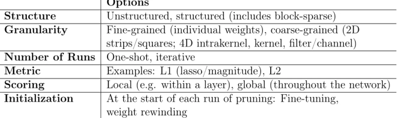
Options
Structure Unstructured, structured (includes block-sparse) Granularity Fine-grained (individual weights), coarse-grained (2D
strips/squares; 4D intrakernel, kernel, filter/channel) Number of Runs One-shot, iterative
Metric Examples: L1 (lasso/magnitude), L2
Scoring Local (e.g. within a layer), global (throughout the network) Initialization At the start of each run of pruning: Fine-tuning,
weight rewinding
Table 4.1: Possible choices while pruning.
Pruning techniques take on a range of granularities from fine-grained (composed of small grains) to coarse-grained (composed of large grains). Unstructured weight prun-ing is the finest-grained technique. In the context of block sparsity, prunprun-ing becomes more coarse-grained the larger the block size. For example, for the 2-dimensional fully connected layers, 32×32 square blocks are more coarse than 4×4 square blocks. 1×32 strips are more coarse than 1×4 strips. In our PyTorch implementation, layers are 2-dimensional tensors in which a weight’s column represents the outbound neuron and row represents the inbound neuron. As a result, removing a strip comprising an entire column or row effectively results in neuron pruning, a highly coarse-grained form of pruning.
Granularity is more complex for convolutional layers, which are represented by 4-dimensional tensors. In increasing structuredness, the block has a dimension for each of:
1. Number of columns (intrakernel). Width within a convolutional kernel. 2. Number of rows (intrakernel). Height within a convolutional kernel. 3. Number of kernels (kernel-level). How many kernels within a filter there
are – for example, for an RGB image, the first convolutional layer may need 3 kernels to handle red, green, and blue.
4. Number of filters (filter-level). Number of filters computed in parallel. Running a filter over activations from the previous layer produces an output
channel. Removing a filter removes an output channel.
A filter-level block is more coarse than a kernel-level block, which is more coarse than row-and-column blocks. Removing an entire filter from a convolutional layer equivalently removes an output channel from that layer, resulting in channel pruning. Just as neuron pruning is a highly coarse-grained form of pruning fully connected layers, so channel pruning is a highly coarse-grained form of pruning convolutional layers.
4.3
Number of Runs
One run involves training the network to completion, then pruning some quantity of weights. In one-shot pruning, all desired weights are pruned in a single run. In contrast, in iterative pruning, some quantity of weights are pruned at each run for a specified number of runs.
4.4
Scoring
To decide which weights to prune, some metric must be used to determine how impor-tant each weight is. A common heuristic is the magnitude of the weight – empirically, weights that have a lower absolute value contribute less to the overall network (the validity of this claim is an open research problem). Other metrics include training importance coefficients and contributions to network activations or gradients.
Determining the importance of a block in block-sparse pruning adds a layer of abstraction. To determine the score of a block in block-sparse pruning, metrics include aggregating the mean (L1/lasso while taking into account padding), sum (L1/lasso), or max of scores within the block.
Once metrics have been chosen, the least important weights are removed. One common practice is to prune a fixed percentage of weights with the lowest scores. Another is to prune values that fall below a specified threshold. Scores may be
compared locally within a subcomponent of the network (such as within a layer), or globally within the entire network.
4.5
Fine-Tuning and Weight Rewinding
It is common practice to fine-tune a network after each run of pruning: at the start of each run, remaining weights take on values of the learned weights from the end of the previous run. An alternative to this implementation is learning rate rewinding [34], which trains the unpruned weights from their final values using the same learning rate schedule as weight rewinding. Renda et al. show that this can match and even outperform fine-tuning, and we use this method as our implementation for fine-tuning. Work related to the lottery ticket hypothesis (discussed in Section 2.1.6) intro-duced the concept of weight rewinding, which alternatively involves rewinding weights to values achieved either at initialization or early in training of the previous run.
4.6
Evaluation
The success of block-sparse pruning can be measured on several levels. Foremost, the goal is to achieve sufficient accuracy at the coarsest granularity. Compared to unstructured weight pruning, in which pruning can be optimized individually at a weight level, imposing a block-sparse structure inherently diminishes the flexibility of pruning. As a result, increased structure would intuitively not increase the accuracy. Finding a balance that maximizes structure while maintaining acceptable accuracy would allow maximum yield of the benefits of block-sparse pruning.
Next, the goal is to maximize computational speedups and memory reductions. Due to increased structure, block-sparse pruning has the potential for greater effi-ciency than unstructured pruning. Ongoing advancements hardware architectures and kernels may allow for increasingly tangible benefits.
Chapter 5
Block Sparsity in Neural Networks
To study the role of block sparsity in neural networks, we focus on two primary ques-tions. The first involves understanding the role of block-sparse pruning at inference time. Question 1: How sparse can we make a network without impacting accuracy, while imposing various block-sparse granularities? We know that the highly structured pruning of neurons and channels obtains notably lower accuracy than unstructured weight pruning, likely due to added structural constraints [2]. The closer the results are to unstructured pruning, the more viably block-sparse pruning can be used to improve network efficiency.
Our second question involves understanding the role of block sparsity at training time. Question 2: With omniscient knowledge of which blocks will end up pruned, would we have been able to prune those weights at the beginning or much earlier in training and yield the same results? This question is motivated by work on the lottery ticket hypothesis, which contends that individual weights can be pruned early in training while maintaining accuracy. Investigating this would allow us to further understand the discrepancy between lottery ticket behavior in unstructured and highly structured neuron and channel pruning and to determine whether it might be possible to train in a block-sparse fashion.
We run two sets of (almost identical) experiments in parallel to answer these questions. For the first question, at each training run, weights are set to the learned weights found at the end of the previous run. This is a fine-tuning procedure
com-monly used in pruning literature [4] [16]. For the second, at each training run, weights are set to values found at initialization or early in training of the previous run. This is the weight rewinding procedure used in lottery ticket work by Frankle et al. [9] [10].
5.1
Methodology
We apply block-sparse pruning to a range of networks by assigning the same impor-tance score to all weights within a block, then iteratively pruning the weights with the lowest scores at each run of training. Chosen block sizes for fully connected lay-ers take one of two shapes: (1) squares with lengths that are powlay-ers of 2 and (2) long strips with side lengths of one and a power of two. For convolutional layers, we prune elements from power-of-two number of kernels at a time and also prune squares and strips from individual kernels. Repeating this procedure for a wide range of granularities allows us to evaluate the effect of increasing block-sparse structure in pruning. Accuracies are directly compared to those achieved by unstructured weight pruning. Comparisons between different block shapes representing equal numbers of weights are also analyzed. Ultimately, the goal is to maximize pruning structure while maintaining a benchmark level of accuracy.
5.1.1
Selection of Benchmarks
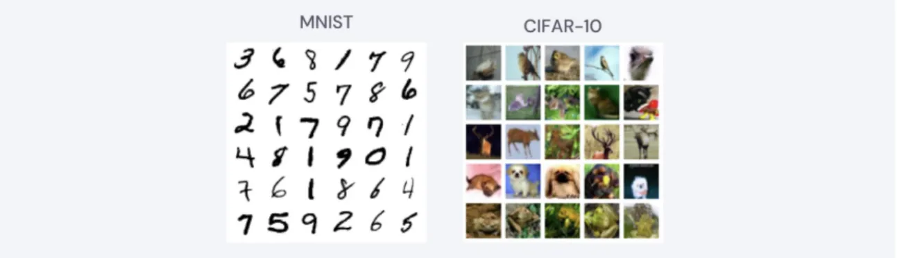
We explore the impact of block sparsity on accuracy on two benchmark tasks: 1. Image classification, black-and-white. We train a LeNet fully connected
model with 256 neurons in each of two hidden layers on MNIST [25], the de facto computer vision dataset with 60,000 28×28 black-and-white images of handwritten digits.
2. Image classification, colored. We train a ResNet-20 [18] on CIFAR-10 [21]. This dataset contains 60,000 32×32 colored images in 10 classes.
Figure 5-1: Benchmark datasets used in image classification. MNIST contains 60,000 black-and-white handwritten digits. CIFAR-10 is a collection of 60,000 images span-ning 10 categories.
5.1.2
Pruning Specifications
We perform block-sparse pruning, removing 20% of the globally lowest-scoring un-pruned weights during each of 15-20 runs. The importance assigned to an individual weight is the mean of weight magnitudes of the block it resides within, which is es-sentially equivalent to the L1 norm after taking into account any padding needed to cleanly divide the layer into blocks. We chose this metric because it is simple to compute, and it is a common heuristic used to determine the amount of impact a given weight has on a network [4].
For weight rewinding experiments, we rewind to initialization for MNIST and 1.5% of the way through pruning for CIFAR-10. These are the specifications used in the original lottery ticket papers [9] [10].
5.1.3
Block-Sparse Shapes
Fully connected layers. Within a fully connected layer, each neuron has a scalar weight associated with each neuron in the next layer. In PyTorch, the values are stored as a 2-dimensional tensor (a matrix). For such layers, we focus on two main block shapes: squares and strips.
• Squares. Though blocks may take on an arbitrary width and height, we focus on square blocks with side lengths that are a power of two, including 2×2, 4×4,
Figure 5-2: Example of block-sparse pruning in fully connected layers. The gray blocks have been pruned, while the blue blocks remain unpruned. We run experi-ments on power-of-two squares and long power-of-two strips. The bottom-right layer contains pruned strips, effectively the equivalent of neuron pruning.
8×8, 16×16, and larger. Using 1×1 block size is equivalent to unstructured weight pruning.
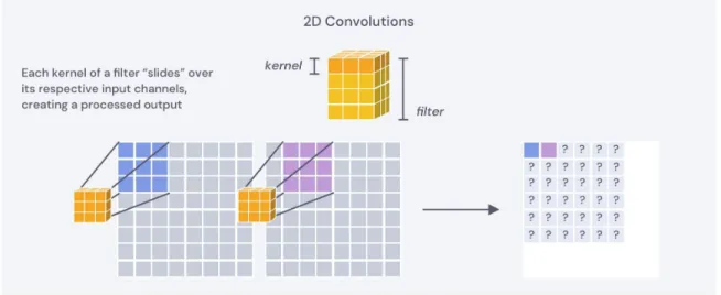
• Strips. We focus on long strips with side lengths of one and a power of two, including 1×2, 1x4, 1×8, 1×16, and longer. Removing an entire column or row from a fully connected layer in practice effectively removes a neuron from the network. Setting weights of an entire row to zero, for example, removes all the inbound weights from a neuron, resulting in neuron pruning. Pruning a 1×16 strip results in the removal of 16 inbound weights coming into one neuron. Convolutional layers. Convolutional layers used by many image classification networks are more complex, as layers are connected via a sliding matrix and images tend to have separate kernels for each incoming channel. This is demonstrated in Figure 5-3. For these layers, weights are stored as a 4-dimensional tensor, Given (typically) 3x3 convolutional kernels and an image, each kernel “slides” over the input channels of the image, performing a computation at each 3×3 window.
Figure 5-3: Convolutional kernel sliding over an image.
Each incoming channel has its own kernel, composing a filter. After doing this, the results of all the filters are added together. Often, several filters are contained within a convolutional layer. This can be seen in Figure 5-4, and describes the hierarchy of structure. For convolutional layers, we focus on two main block shapes:
• Varying number of 1×1 blocks within multiple consecutive kernels. Corresponding elements from 2, 4, 8, 16, and longer contiguous kernels form a block.
• Intrakernel 1×3, 3×1, 3×3 blocks. The networks we run experiments on contain kernels of size 3×3. We examine pruning rectangular strips within a kernel (1×3, 3×1) as well as removing entire kernels at a time (3×3).
5.2
Block Sparsity Implementation
We utilize a PyTorch implementation for our neural network models. In PyTorch, weight parameters are stored in a Python dictionary in which keys are unique iden-tifiers of a layer, and values are multidimensional PyTorch tensors representing the weights of that layer. Fully connected layers are 2-dimensional while convolutional layers are 4-dimensional.
Figure 5-4: 4D representation of convolutional layer weights. Each kernel is made of columns and rows. A filter is made of several kernels. There are several filters within a convolutional layer.
For each weight in a layer tensor, we want to assign an importance score to determine whether the weight should be pruned. To accomplish this, we create a corresponding tensor of the same shape containing importance scores. Given a block shape, our implementation performs the following steps:
1. A layer may have a shape that is not cleanly divisible by the block shape. In this case, our implementation pads the weights with just enough zeros in all applicable dimensions such that each side length is divisible by its corresponding block side length. The padded layer is stored in a temporary variable.
2. Arrange the padded weights conveniently to allow for a grouping of weights into blocks.
3. Calculate the importance value for each block by taking the aggregate mean of the absolute values of weights within that block.
4. Broadcast this score such that there exists a score for each weight in the original padded matrix.
5. Reshape such that scores take the shape of the original padded matrix. In the resulting tensor, each element should take the value of the aggregate score of the block the original element was located in.
6. Remove the added padding from the matrix by slicing the tensor.
Now that each weight is assigned an importance score, we prune 20% of the lowest-scoring unpruned weights at each run of pruning. A layer is pruned by applying a mask 𝑀 to its weights 𝜃′. The mask is 1 for unpruned weights and 0 for pruned
weights. The elementwise product of the two, 𝑀 ⊙ 𝜃′, then has the weight values of
𝜃′ with pruned weights set to zero.
5.3
Results
We compare the accuracy achieved by unstructured pruning to those achieved by structured pruning with various block granularities. We then compare between block shapes containing the same number of weights to evaluate whether there exist specific block shapes that can maintain accuracy.
Fine-tuning. These experiments provide insight into answering our two primary questions. There are several potential behaviors we may expect. Question 1: How sparse can we make a network without impacting accuracy, while imposing various block-sparse granularities? We use a fine-tuning procedure by setting weights to learned values from the previous run. There are two possible outcomes:
• Block-sparse pruning is unable to maintain the same accuracy at the same percentage pruned as unstructured pruning. Since the maximum possible accuracy is not attainable at this block granularity, we should consider the tradeoff between accuracy and efficiency when deciding whether to apply block-sparse pruning at this block shape and size.
• Block-sparse pruning maintains the same or better accuracy at the same percentage pruned as unstructured pruning. This would be the best-case scenario because it would mean that we can add structure to the network without compromising accuracy. There is potential that pruning with this block shape can be used in place of unstructured pruning for efficiency benefits – further considerations include whether the block size is large enough
to take advantage of memory and computation benefits and which block shape of the same effective size yields the highest accuracy. Such an outcome would be particularly interesting because it has already been shown that pruning entire neurons and channels results in lower accuracy than unstructured pruning. Weight rewinding. We next address our second question regarding lottery ticket behavior in block-sparse pruning. Question 2: With omniscient knowledge of which blocks will end up pruned, would we have been able to prune those weights at the beginning or much earlier in training and yield the same results? We test this by rewinding unpruned block weights to values from initialization or early in training of the previous learning run. For a given block size and shape, there are several possible outcomes:
• Rewinding weights to values early in training, the resulting network cannot match the accuracy of the full network at the same percentage pruned as unstructured pruning. This means that we cannot constrain unpruned weights with this block structure and expect the network to learn to the same accuracy earlier in training. Perhaps at this block granularity, we can match the accuracy of the full network only when fewer weights are pruned. • Rewinding weights to values early in training, the resulting network
matches or exceeds the accuracy of the full network at the same per-centage pruned as unstructured pruning. This would offer evidence that block-sparse pruned networks exhibit lottery ticket behavior – we can train the resulting block-sparse network (which takes on values found early in training) and expect the network to learn to the same accuracy as the full network. Such a finding would be particularly exciting, as it shows that structural constraints can be added to a network and it would still be able to learn with informa-tion learned early in training. Though exceeding accuracy would be a pleasant finding with potential to improve upon state-of-the-art pruning methods, this is inconsistent with the behavior of unstructured weight pruning and highly unlikely due to increased constraints imposed by block sparsity.
5.3.1
Experiments
We run experiments on two image classification benchmarks, with two settings per benchmark: fine-tuning and weight rewinding. To determine what accuracy can be achieved given a block size and shape, we fine-tune the network at each run by using values learned in the previous training run. Then, to determine whether this accuracy could have been achieved given omniscient knowledge, we run an additional experiment in which we rewind the weights to values attained early in training during the previous run.
MNIST
Fine-Tuning Weight Rewinding
1×1 5.5% 5.5% 1×2 6.9% 5.5% 1×4 6.9% 5.5% 1×8 6.9% 5.5% 1×16 13.4% 8.6% 1×32 13.4% 13.4% 1×64 32.7% 20.9% 2×2 13.4% 6.9% 4×4 13.4% 6.9% 8×8 13.4% 6.9% 16×16 32.6% 32.6% 32×32 40.6% 32.6% 64×64 78.7% 48.2%
Table 5.1: Percent of weights remaining at the maximum sparsity attainable while maintaining accuracy of the full network. We prune with various block shapes on fully connected LeNet trained on MNIST benchmark.
We evaluate Question 1: How sparse can we make a network without impacting ac-curacy, while imposing various block-sparse granularities? Table 5.1 lists the number of weights remaining at the maximum sparsity at which the network can be pruned without reducing accuracy. We can see that there are 5.5% of weights remaining for unstructured pruning at the maximum sparsity attainable by fine-tuning. This is not matched by any block size in our fine-tuning experiments. As a result, we conclude
Figure 5-5: Effect of varying block granularity on accuracy for fully connected LeNet trained on MNIST benchmark. Left: Networks with fine-tuning. Right: Networks with weight rewinding (lottery ticket). Blocks are long strips with a power-of-two side length (top) or squares with power-of-two side lengths (bottom).
that there is a tradeoff between block size and accuracy: we cannot benefit from block structure without compromising accuracy.
We then investigate Question 2: with omniscient knowledge of which blocks will end up pruned, would we have been able to prune those weights much earlier in training and yield the same results? We can see that the 5.5% of weights remaining attainable by unstructured pruning can only be matched only by small blocks of up to 1×8 in our weight rewinding experiments. As a result, we conclude that we cannot maintain accuracy while using values early in training to the same sparsity as unstructured pruning.
There are several additional observations that can be made. As seen in Figure 5-5, accuracy tends to decrease as block size increases across experiments. This drop in accuracy begins some point after a significant percentage of weights have already been pruned. In addition, this drop is gradual rather than sharp for smaller block sizes. For larger block sizes such as 16×16 and 32×32, Figure 5-5 makes clear a notably sharp drop at lesser sparsities.
The data offers evidence that weight rewinding can reach slightly greater sparsities than fine-tuning. Fine-tuning cannot match the 5.5% of weights remaining achieved by unstructured pruning, but can achieve a close 6.9% of weights remaining up to a 1×8 block size. Weight rewinding can match 5.5% for a block size of up to 1×8, can achieve 8.6% of weights remaining for the next 1×16 block size. Indeed, it is worth noting that there is a significant dip in 16×16 block accuracy at a lesser sparsity for fine-tuning than for weight rewinding.
CIFAR-10
We now evaluate Question 1 on CIFAR-10. Table 5.2 shows that any choice of block leads to lower maximum sparsities than the 13.4% of weights remaining in unstruc-tured pruning. We conclude that there is a similar tradeoff between block size and accuracy: we cannot benefit from block structure without compromising some amount of accuracy.
Figure 5-6: Effect of varying block granularity on accuracy for ResNet-20 trained on CIFAR-10 benchmark. Left: Networks with fine-tuning. Right: Networks with weight rewinding (lottery ticket). Blocks are composed of 1×3, 3×1, 3×3 blocks within a single kernel (top) or 1×1 squares power-of-2 kernels at a time (bottom).
Fine-Tuning Weight Rewinding [1×1]×1 13.4% 16.8% [1×3]×1 21.0% 26.2% [3×1]×1 21.0% 26.2% [3×3]×1 26.2% 64.0% [1×1]×2 16.8% 21.0% [1×1]×4 21.0% 32.8% [1×1]×8 21.0% 64.0% [1×1]×16 21.0% 64.0%
Table 5.2: Percent of weights remaining at the maximum sparsity attainable by prun-ing with various block shapes for ResNet-20 trained on CIFAR-10 benchmark.
find that there is no block structure that does not need some compromise in accuracy. We conclude that we cannot impose block-sparse structure and expect to find sparse networks early in training that can reach the sparsity of unstructured pruning.
By analyzing Figure 5-6, we make additional observations. Similar to MNIST, accuracy tends to decrease as block size increases, beginning after a significant per-centage of weights have already been pruned. The drop in accuracy is gradual for smaller block sizes, and only becomes pronounced with larger blocks such as [1×1]×16. The difference in test accuracy between fine-tuning and weight rewinding is more pronounced for CIFAR-10. Fine-tuning weights results in accuracies higher than rewinding weights, contrary to our observations for MNIST in which accuracies are slightly lower. For example, at 5.5% of weights remaining, 3×3 blocks achieve 87% accuracy with fine-tuning and 84.5% accuracy with weight rewinding. At 5.5% of weights remaining, [1×1]×8 blocks achieve 88% accuracy with fine-tuning and 85% accuracy with weight rewinding. These observations offer evidence that fine-tuning is preferable to weight rewinding in block-sparse pruning. Another interesting note is the dramatic drop in accuracy for [1×1]×16 blocks at roughly 6.9% sparsity, which is found in fine-tuning but not weight rewinding.
Figure 5-7: Comparison of block shapes in fully connected layers, for fully connected LeNet trained on MNIST benchmark. Long strips and square blocks containing equal numbers of weights are compared. Left: Networks with fine-tuning. Right: Networks with rewinding (lottery ticket).
5.3.2
Long Strips vs. Square Blocks
Long strips and square blocks are our shapes of choice for fully connected layers. Prun-ing long strips involves removPrun-ing many weights from a sPrun-ingle neuron, while prunPrun-ing square blocks involves removing an equal number of weights from several neurons. We are interested in understanding which shape is preferable for maximizing accu-racy, as this would provide insight into which shape to use to maximize accuracy at the same sparsity. From the existing literature, we know that large-sparse networks outperform small-dense networks [41]. As a result, we might expect that a pattern in which zero-valued weights are scattered would perform better than one in which an entire row or column are pruned.
To compare between the efficacy of the two, we analyze our LeNet fully connected model for MNIST experiments on blocks containing the same number of weights – pairing 1×4 with 2×2, 1×16 with 4×4, 1×64 with 8×8, and 1×256 with 16×16. From the results shown in Figure 5-7, we observe that square blocks obtain notably higher accuracy than long strips containing the same number of weights. The difference between the two is not large; however, it becomes more pronounced as block size is increased. This is consistent with our hypothesis that pruning scattered weights leads to higher accuracy than pruning entire rows and columns.
5.3.3
Intrakernel vs. Kernel-Level Blocks
In convolutional layers, we experiment with intrakernel blocks and blocks spanning several kernels. Again, we are interested in understanding how shape plays a role in maximizing accuracy at the same sparsity. Convolutional kernels are often 3×3, so we consider intrakernel blocks of 1×3, 3×1, and 3×3. Pruning a 3×3 intraker-nel block equivalently removes an entire kerintraker-nel from the network. We also use 1×1 blocks spanning power-of-two kernels at the same time. For example, we consider [1×1]×2, [1×1]×4, [1×1]×8, and [1×1]×16 blocks. Though it is possible to experi-ment on longer kernel blocks, these longer blocks may not represent quantities that are meaningful in practice. Since large-sparse networks perform better than
small-Figure 5-8: Compares varying intrakernel block shapes to varying block kernel depth. Equal numbers of weights are compared. Left: Networks with fine-tuning. Right: Networks with rewinding (lottery ticket).
dense networks, we might expect that a pattern in which zero-valued weights are scattered would perform better than one in which an entire convolutional kernel is pruned.
We analyze results from our ResNet-20 convolutional model for CIFAR-10 exper-iments on blocks containing the same number of weights. Since there are a small, countable number of possible intrakernel blocks, we specifically compare blocks with 3 weights and blocks with 9 weights. Results are displayed in Figure 5-8. For blocks with 3 weights, intrakernel and kernel-level blocks reveal similar accuracy. For blocks with 9 weights, removing 9 kernel-level blocks obtains notably higher accuracy than removing entire 3×3 convolutional kernels. Similar to MNIST, this is consistent with our hypothesis that a scattered pruning arrangement is preferable to removing entire functional components of the network.
5.4
Discussion
Neuron and channel pruning have been shown to have significantly lower accuracy than unstructured weight pruning at the same sparsity [29]. At the same time, un-structured pruning is more difficult to accelerate than un-structured pruning. Our work was motivated by the question of whether there exists a structured pruning method that can maintain accuracy while improving computational efficiency. Our experi-ments demonstrate that block sparsity does appear to be a reasonable medium be-tween the extremes. Increasing block size results in a gradual decrease in accuracy, rather than a sharp drop occurring when at neuron or channel levels of structure. At the same time, using block sparsity is not tradeoff-free. Block sparsity is unable to maintain accuracy at the same percentage pruned as unstructured pruning for all but the smallest of tasks (up to a 1×8 block size in our MNIST weight rewinding experi-ments). As a result, the viability of block-sparse pruning involves a tradeoff between granularity and accuracy. For real-world cases, it may be useful to find a balance between computational and memory needs and accuracy depending on priorities.
of which blocks would end up pruned. This would mean that it is possible to add structural constraints to a network and still be able to learn from early in training. Such a discovery would run parallel to lottery ticket behavior examined by Frankle et al. [9] in unstructured weight pruning. The weight rewinding experiments inspired by the lottery ticket hypothesis reflect this question. Our experiments on MNIST and CIFAR-10 demonstrate that adding any amount of block structure results in a reduced accuracy when compared to unstructured pruning (with the exception of equal accuracy obtained by 1×8 block in MNIST weight rewinding).
Though we find that weight rewinding has a neutral and slightly beneficial impact on accuracy compared to fine-tuning for MNIST, it seems to have a notably negative impact on accuracy for CIFAR-10. Because ResNet-20 on CIFAR-10 is a much larger task than fully connected LeNet on MNIST, we believe that results on CIFAR-10 are more representative of image classification tasks as a whole. As a result, it seems that lottery ticket behavior may not hold in block-sparse pruning.
Finally, we find that square blocks outperform long strips with the same number of weights, and small blocks spanning several kernels outperform removing entire sec-tions from convolutional kernels. This is not an obvious finding – however, it seems reasonable that removing a few connections from many neurons/channels results in better accuracy than removing most or all connections from a few neurons/channels. This is consistent with past findings that the scattered pattern of large-sparse net-works outperform the localized pattern of small-dense netnet-works.