MAD workshop - November 4th, 2014
The synergy between
optical interferometry
and imaging
Olivier Absil
Outline
❖
Imaging vs. interferometry
❖
Similarities, differences
❖
Synergy: illustrations
❖
Protoplanetary disks
❖
Debris disks
❖
Extrasolar planets
Wachowski & Wachowski 1999
Imaging vs.
Two names for one phenomenon
❖
Diffraction+interference at the root of image formation
The borders of their realms
❖
Angular resolution: λ/2B
❖
Field-of-view limited by
bandwidth smearing
and/or use of fibers
B
D
❖
Angular resolution:
Where’s the limit?
A continuum of angular resolution
0.001’’ 0.01’’ 0.1’’ 1’’ 10’’
NIR interfero
NIR imaging
NIR aperture masking
E-ELT masking
E-ELT imaging
ALMA
Image or model?
❖
Image: constrains the surface brightness
❖
Forward modelling: constrains model parameters
Model or image?
❖
Model-fitting interferometric observables (V2, CP)
❖
Image reconstruction: surf. bright. / forward modeling
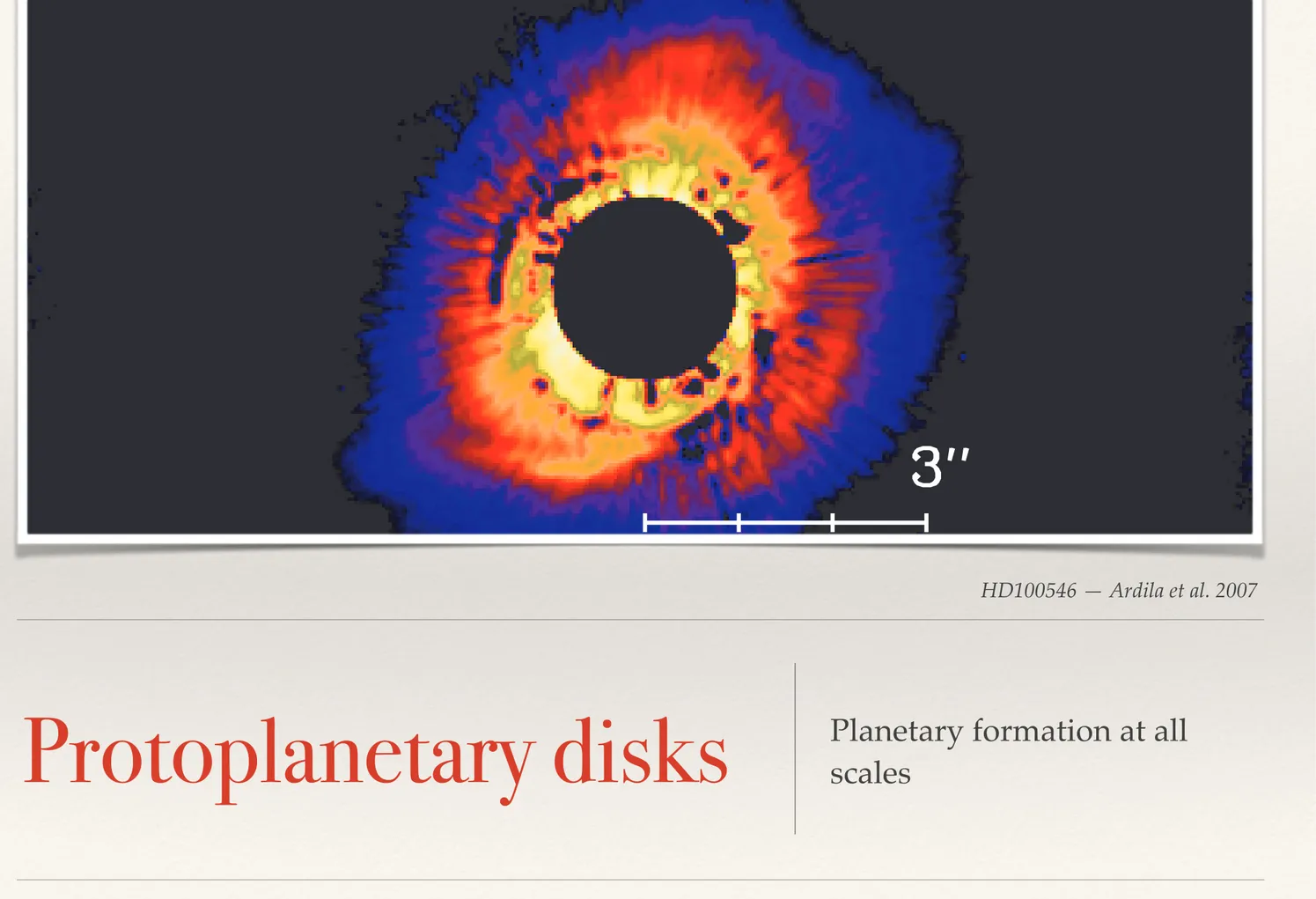
HD100546 — Ardila et al. 2007
were minimized. The uncertainty in the registration of the
im-ages along each axis is 0.125 pixels. For the normalization
con-stants we performed the following visual, iterative adjustment.
Starting with the flux ratios implied by the values from Table 2
(0.391, 0.443, and 0.474 for F435W, F606W, and F814W,
re-spectively), we adjusted the scaling until the subtraction residuals
were minimized. This occurred for normalization constants 0.383,
0.382, and 0.387 in F435W, F606W, and F814W, respectively.
Visually, the uncertainty of these normalization values is 3%, and
in what follows we propagate this error linearly (as a systematic
error) to estimate uncertainties in calculated quantities (
x 3.4).
The values of the normalization constants are consistently lower
than implied by the values quoted in Table 2, as expected by the
mismatch between the colors of the PSF reference star HD 129433
and those of its spectral model.
After subtracting the coronagraphic images of HD 129433
from each image of HD 100546, we corrected for the geometric
distortion in the HRC image plane, using the coefficients of the
biquartic polynomial distortion map provided by STScI ( Meurer
et al. 2002) and cubic convolution interpolation to conserve the
imaged flux. By using standard IRAF routines, we aligned the
two rolls in each band, using other stars in the field for reference,
Fig. 1.— Surface brightness maps of the circumstellar environment of HD 100546, in a logarithmic stretch. All images have been normalized to the stellar brightness in
their respective bands. The approximate size of the coronagraphic mask is shown as a black circle 1
00
in radius. The top row has a different color stretch and spatial scale than the
other two, in order to showcase different regions. The top stretch goes from 10
!7
to 10
!3
arcsec
!2
. The middle and bottom rows show a stretch from 10
!5
to 10
!3
arcsec
!2
.
The contours in the bottom row are obtained from images that have been heavily smoothed. The contour values are (2
; 3; 4; 5; 6; 7; 9; 12; 15) ; 10
!5
arcsec
!2
.
ARDILA ET AL.
516
Vol. 665
Protoplanetary disks
Planetary formation at all
Synergy in a nutshell
Their observations trace gas at distances<100 AU from the star. Assuming that the disk rotates in the same direction at larger dis-tances from the star and that the southwest side is oriented to-ward the Earth (x 3.4.2), those spectral observations indicate that the structures are trailing the direction of rotation.
Before deconvolution, the behavior of the structures with wavelength is tangled with the changing resolution of the tele-scope at different passbands ( Fig. 1). The deconvolved images ( Fig. 3) reveal no obvious morphological differences in each band, for each of the structures. The contour levels traced on the de-convolved images show that the space between the inner part of
the disk and the structures becomes brighter at longer wave-lengths, while the value of the peak brightness does not change much between bands. This color behavior is discussed inx 3.4. The circumstellar disk is illuminated by the starlight, which decays as the inverse distance squared from the star. An appro-priate correction for this effect is only possible for face-on disks. We therefore deproject the disk by the inclination, divide by the Henyey-Greenstein scattering phase function withg¼ 0:15 (de-rived inx 3.4.2), and multiply every pixel by the square of the projected distance to the star. This procedure will reveal the cor-rect geometry and brightness of the circumstellar material only
Fig. 7.— Unsharp masking of the nondeconvolved image in the F435W band. Top left: Deprojected image, with each pixel corrected by scattering asymmetry (g¼ 0:15) and multiplied by !2, where! is the angular distance to the star. Notice that the hemispheric subtraction residuals are circular in the original image, so they look
elliptical here. Top right: Same image, smoothed by a Gaussian kernel with 30 pixels FWHM. Bottom left: Unsharp masking, the result of subtracting the top right image from the top left. Bottom right: Same as bottom left, with features identified. We only mark those features that are identified in all the bands. Features 1a, 2a, and 3a correspond to structures 1, 2, and 3 in Fig. 6.
HST ACS OBSERVATIONS OF HD 100546 521 No. 1, 2007
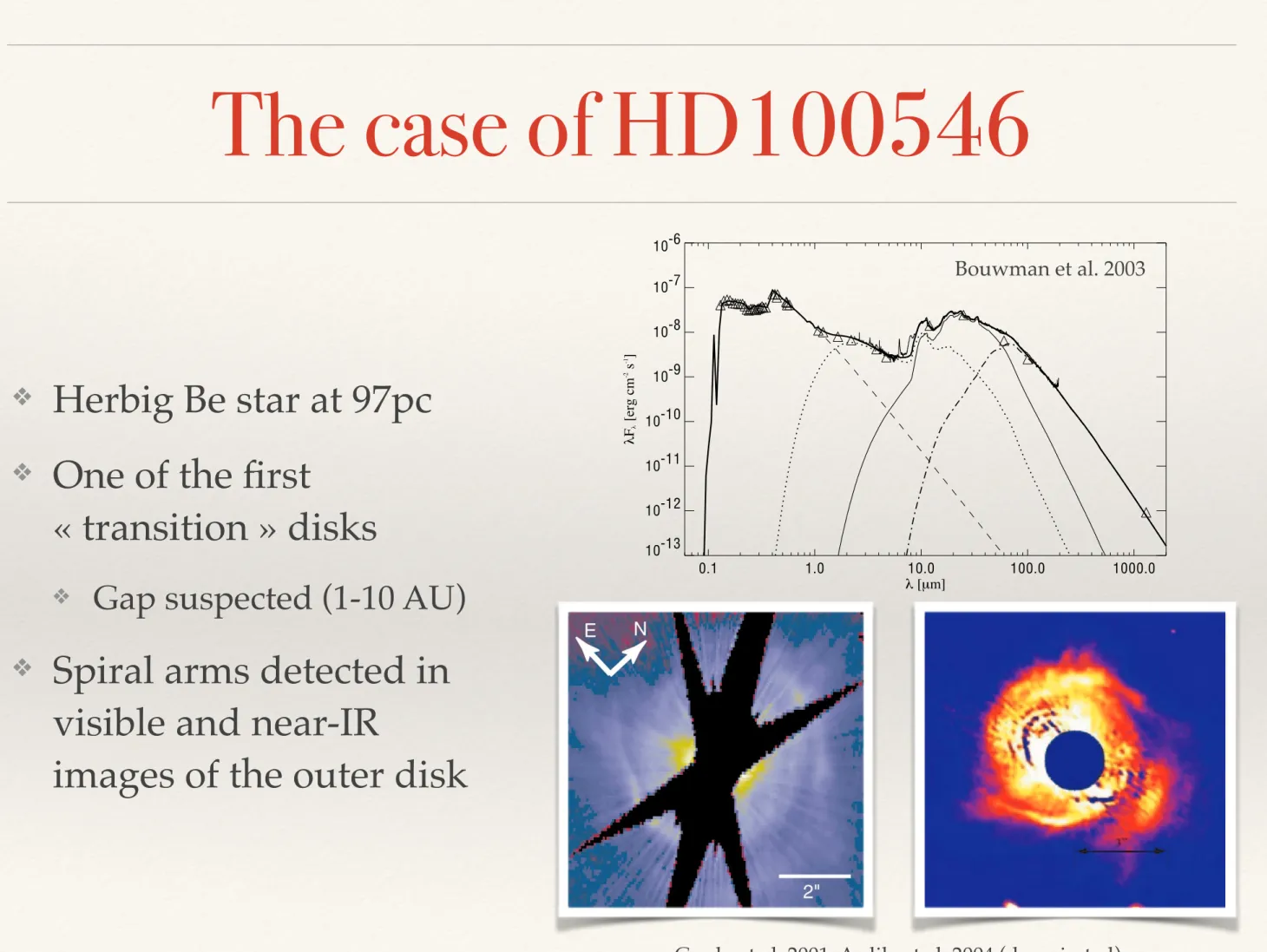
The case of HD100546
❖
Herbig Be star at 97pc
❖
One of the first
« transition » disks
❖
Gap suspected (1-10 AU)
❖
Spiral arms detected in
visible and near-IR
images of the outer disk
J. Bouwman et al.: HD 100546 583 0.1 1.0 10.0 100.0 1000.0 λ [µm] 10-13 10-12 10-11 10-10 10-9 10-8 10-7 10-6 λ Fλ [erg cm -2 s -1 ] 10 100 λ [µm] -100 0 100 200 300 Fν [Jy] Ol Fo 2 3 4 5 6 7 8 λ [µm] 0 2 4 6 8 10 Fν [Jy]
Fig. 2. The top panel shows our best model fit to the spectral energy
distribution of HD100546 (thick solid line). Indicated with the dashed line is the spectrum of the central star. Triangles indicate ground-based and IRAS photometry. Also plotted are the the ISO-SWS and LWS spectra. The dotted line, the thin solid line and the dashed-dotted line represent the contributions of the small grain components in zone 1, zone 2 and the large grain component, respectively. The bottom panel shows our fit to the ISO spectra in detail. Also plotted in this fig-ure are the relative contributions of the individual dust components. Indicated with a solid line are the contributions of amorphous olivine and forsterite marked in the figure with Ol and Fo, respectively. The contribution of water ice, carbonaceous grains and metallic iron are represented by the dashed, dotted and dashed-dotted lines, respec-tively. The curves of the carbonaceous, forsterite and metallic iron grains are o↵set by 40, 75 and 90 Jy, respectively. The inset shows the 2 to 8 µm region.
size required to fit the slope of the SED at mm wavelengths. There are however some problems with the 60 µm band as we will discuss in Sect. 4.1.5.
We have constrained the spatial extent of the large grains using the disk size observed by Augereau et al. (2001) with the HST/NICMOS2 instrument. To fit the observations, a gap of 28 AU is required between the central star and the dust shell containing the large grains. As noted in previous stud-ies (Bouwman et al. 2000), this gap is most likely an artifact of the assumption made in this study that the medium is opti-cally thin in the radial direction. In HD 100546 we see the disk fairly face on (51 Augereau et al. 2001), implying that in the line-of-sight the medium may well be optically thin. Therefore,
21
22
23
24
25
26
λ [µm]
0
10
20
30
40
F
ν[Jy]
31
32
33
34
35
36
37
38
λ [µm]
0
10
20
30
40
50
60
F
ν[Jy]
Fig. 3. The 24 and 34 µm forsterite bands of HD 100546. Overplotted
are the best fit silicate bands using the data of Servoin & Piriou (1973) (solid line), Steyer (1974) (dotted line) and Mukai & Koike (1990) (dashed line). In the latter model spherical grains were assumed with a size of 0.01 µm. The other models have a CDE shape distribution.
the derived mass over temperature distribution Td(m) remains meaningful (albeit not the Td(r) structure). As suggested by Bouwman et al. (2000) the large grains have most likely settled to the disk mid-plane, extending all the way to the disk inner edge. Recent full 2D radiative transfer calculations (Bouwman 2001) confirm this qualitative picture. These calculations also show that the Td(r) of the hot small grains, residing in the op-tically thin surface layer of the disk, is in agreement with the simple spherical optically thin model adopted in this paper. 4.1.4. The mass temperature distribution
The SED as presented in Fig. 2 is determined by the mass-temperature distribution of the circumstellar dust. Irrespective of the assumed model geometry, this distribution has to be re-produced for dust that is contributing to the observed emission features. Plotted in Fig. 5 is the derived mass over tempera-ture distribution of the best fit model. The upper two panels show the mass-temperature distribution of the small grain com-ponent, the lower panel shows the same for the large grains. Indicated in the figure are the individual contributions of each species. The vertical axis unit is chosen in such a way that the integral of the cumulative mass-temperature distribution equals the total dust mass. We have plotted in Fig. 4 the relative con-tribution to the SED of the individual dust species to get a feel-ing of their importance to the overall fit. Plotted in Fig. 6 for comparison is the mass-temperature distribution of AB Aur as derived by Bouwman et al. (2000). The first panel shows the
Grady et al. 2001, Ardila et al. 2004 (deprojected) Bouwman et al. 2003
No. 6, 2001 MULTIWAVELENGTH IMAGING OF HD 100546 3399
FIG. 1.ÈSTIS imagery of the HD 100546 system: (a) Reduced STIS data prior to PSF subtraction, displayed in false color with a logarithmic stretch. The upper image shows the data taken at P.A.\ 17¡.3,with the data from P.A.\ 27¡.3below. TheHST ] STIS PSF dominates the raw data. (b) Same data as (a), following PSF subtraction. Nebulosity can be traced from0A.5 out to 10A from the star at all position angles, and additional nebulosity running from northwest down to southeast can be marginally detected. (c) A 30A ] 25A Ðeld containing HD 100546 data from both spacecraft orientations combined. The irregular polygons in the image are due to voids in the data coverage due to the combined e†ects of the stellar di†raction spikes and the STIS coronagraphic wedge structure. (d) Clumpy structure on 1È2A scales revealed after Ðltering the image from (c) by r2, as has been done for AB Aur (Grady et al. 1999). (e) 4A ] 4A detail of image (c) showing structure in the inner disk. ( f ) After rotating the data from (e) to place the region of maximum elongation horizontal, the deprojected image, assuming a system inclination of 49¡.
(V \ 9.98 mag, K \ 7.98 mag) were taken with the star displaced by ^3A with respect to the mask. The reference-star observations were interleaved with those of the target by using the same AO setup (temporal bandwidth, number
of corrected modes, etc.). This is done to ensure stable system performance, as long as the di†erences in brightness and color of the science target and the reference stars are small and atmospheric conditions are stable. ESO
meteo-NIR interferometry
❖
Tenuous inner disk of small grains, peaking at 0.25 AU,
coplanar with outer disk
❖
Gap confirmed up to 13 AU, possibly opened by planet
❖
Inner disk rim probably not puffed up
MIR interferometry
❖
Sensitive to warm dust, including
inner rim of outer disk
❖
Inner rim = (asymmetric) bright
ring at 11±1 AU
❖
Curvature of inner wall constrained
❖
Hydro simulations suggest massive
gap-clearing BD
❖
Upper limit of 0.7 AU for innermost
disk
Mulders et al. 2013
Vertical wall Round wall
Polarimetric differential imaging
❖
Disk resolved down to
0.1’’ (10AU) with NACO
❖
Outer radius of inner gap
constrained to 14±2 AU
❖
Asymmetric brightness profile
along minor axis (preferential
backward scattering)
❖
Polarization degree suggests
grains larger than ISM grains
❖
Possible hole
High contrast imaging
❖
L-band coronagraphy reveals compact emission at 0.48’’
❖
Deprojected separation ~ 68 AU
❖
Position corresponds to polarimetric hole
❖
Contrast ~ 9 mag
❖
Slightly extended
❖
Possible forming
planet?
Big picture
Fomalhaut — Kalas et al. 2005
Outer disk
24µm
70µm
A double inner disk
Absil et al. 2009 Mennesson et al. 2013 Lebreton et al. 2013VLTI, K band
KIN, N band
K band
N band
Spin-orbit alignment
Consequence on the grains
10µm
30µm
100µm
pure reflectance function
forward
backward
Min et al. 2010
measurement
(Kalas et al. 2005)
beta Pic — Absil et al. 2013
Substellar / planetary
The interferometric view
❖
Double fringe packet
❖
How to measure the phase?
B
"
The closure phase
❖
Closure phase not affected by telescope-specific errors
❖
ψ123 = φ12
+ε
1
+ φ23 + φ31
−ε
1
❖
Not biased by turbulence
❖
Asymmetric objects: ψ
123
≠ 0
❖
Sensitive to companions
❖
ψ123 = ρ (sin α12+sin α23+sin α31)
❖
proportional to flux ratio
❖
![Risiko- & [und] Schutzfaktoren der psychischen Gesundheit humanitärer Einsatzhelfer : eine systematische Literaturübersicht](data:image/gif;base64,R0lGODlhAQABAIAAAP///wAAACH5BAEAAAAALAAAAAABAAEAAAICRAEAOw==)