Detection and localization of link-level network anomalies using end-to-end path monitoring

HAL Id: tel-00860397

https://tel.archives-ouvertes.fr/tel-00860397

HAL is a multi-disciplinary open access archive for the deposit and dissemination of sci-entific research documents, whether they are pub-lished or not. The documents may come from teaching and research institutions in France or abroad, or from public or private research centers.

L’archive ouverte pluridisciplinaire HAL, est destinée au dépôt et à la diffusion de documents scientifiques de niveau recherche, publiés ou non, émanant des établissements d’enseignement et de recherche français ou étrangers, des laboratoires publics ou privés.

Detection and localization of link-level network

anomalies using end-to-end path monitoring

Emna Salhi

To cite this version:

Emna Salhi. Detection and localization of link-level network anomalies using end-to-end path moni-toring. Other [cs.OH]. Université Rennes 1, 2013. English. �NNT : 2013REN1S021�. �tel-00860397�

*+,-$%.%/"01$2-0*#%3$%2$""$-%(

!"#!$%&$!'&(#$)&$%*+,-.&/!-01$2#/"31&,,&$)&$4/&0(5,&

!"#$%&'%($)*'%*'

345*$/2%3$%67/"01$2-0*#%3$%2$""$-%(

6&,0-",$7$8,9"/:(0-;#&

$89:;%<98=9>?:;%@!*0--$

!$+,'-.+'%!)$

$AB?%-?:CD

/$+!)$+'%0%&1#-2.+%*'%$'34'$34'%56578

%

!"#$%$&$'()'*)+,)-+,)')"'!"./-01$%2&)')$'34#$50)#'6781$/%-)#

9/0:/#1"$)';"%<)-#%$1%-)='!3>!9

%

%%%%%%%%

%

%

%%

%

%%%%%%%%

%%

%

%%%%%%%%

%%

%%%%%%%%

%%

%

%%%%%%%%

%%

%

%%%%%%%%

%%

%

%

%%%%%%%%

%%

%%%%%%%%

%%

%

%%%%%%%%

%%

%

%%%%%%%%

%%

%

%%%%%%%%

%%

%

%%%%%%%%

%

0B=D=E:F%<;%:?%=CGH;I

3;=;8=D9B%?B<%

698?:DJ?=D9B%9K%6DBLM

6;N;:%";=O9>L%

!B9A?:D;H%/HDBP%

$B<M=9M$B<%Q?=C%

@9BD=9>DBP%

*CGH;%H9E=;BE;%R%2;BB;H

:;%()S'&S&'()

QCD:DTT;%4O;J?>HLD

!BE>?%QS%U?V?HEA?B?

-?B<>DB;%1?=9B

@DL:9H%@9:B?>

W;>B?><%59EHDB

-?A;>%6?C9E<

Abstract

This thesis investigates the problem of link-level anomaly detection and localization using end-to-end path monitoring. The aim is to come up with cost-efficient, accurate and fast schemes for link-level network anomaly detection and localization. The anomaly detection aims at detecting the occurrence of anomalies in the network (e.g., excessive delays, high loss rate, infrastructure failures, etc.) and identifying a set of links suspect to be the source of the anomaly. The anomaly localization is triggered upon detecting an anomaly. It aims at reducing the set of suspect links identified by the detection process to the anomalous link(s).

It has been established that, for detecting all potential link-level anomalies, a set of

paths that cover all links of the network1

must be monitored, whereas for localizing all potential link-level anomalies, a set of paths that can distinguish between all links of the

network pairwise2

must be monitored. Either end-node of each path monitored must be equipped with a monitoring device.

Most existing link-level anomaly detection and localization schemes are two-step. The first step selects a minimal set of monitor locations that can detect/localize all potential link-level anomalies. The second step selects a minimal set of monitoring paths between the selected monitor locations such that all links of the network are covered/distinguishable pairwise. However, such step-wise schemes do not consider the interplay between the conflic-ting optimization objectives of the two steps, which results in sub-optimal consumption of the network resources and biased monitoring measurements. One of the objectives of this thesis is to evaluate and reduce this interplay. To this end, one-step anomaly detection and localization schemes that select monitor locations and paths that are to be monitored

1. A link is said to be covered if it is traversed by at least one monitoring path

2. Two links are said to be distinguishable if we are able to decide which one is anomalous when an anomaly occurs on one of them

jointly, thereby achieving a good trade-off between the number and locations of monitoring devices and the quality of monitoring paths, are proposed

Furthermore, we demonstrate that the already established condition for link-level ano-maly localization is sufficient but not necessary. A necessary and sufficient condition that minimizes the localization cost drastically is established.

The problems are formulated as integer linear programs and are demonstrated to be N P-Hard. Scalable and near-optimal heuristic algorithms for anomaly detection and ano-maly localization are proposed. The effectiveness and the correctness of the proposed schemes and algorithms are verified through theoretical analysis and extensive simulations.

Key Words : Network monitoring, anomaly detection, anomaly localization,

Résumé en français

Cette thèse étudie le problème de la détection et de localisation des anomalies au niveau des liens en utilisant un monitorage des chemins de bout-en-bout. L’objectif est de trouver des techniques de détection et de localisation des anomalies au niveau des liens qui soient à faible coût, précises et rapides. La détection d’anomalies vise à détecter l’apparition d’anomalies dans le réseau (par exemple des retards excessifs, un taux de perte élevé, des pannes d’infrastructure, etc) et d’identifier un ensemble de liens soupçonnés d’être la source de cette anomalie. La localisation des anomalies est déclenchée en cas de détection d’une anomalie. Elle vise à réduire l’ensemble des liens suspects identifiés par le processus de détection d’anomalies au(x) lien(s) défaillant(s).

Il a été établi que pour détecter toutes les anomalies possibles au niveau des liens d’un réseau, un ensemble de chemins qui couvrent tous les liens du réseau 3 doit être monitoré, alors que pour localiser toutes les anomalies potentielles au niveau des liens d’un réseau, un ensemble de chemins qui peuvent distinguer entre tous les liens du réseau paire par paire 4 doivent être monitorés. Chaque nœud d’extrémité de chaque chemin monitoré doit être équipé d’un dispositif de monitorage.

La plupart des techniques de détection et de localisation des anomalies au niveau des liens qui existent dans la littérature calculent les solutions, c-à-d l’ensemble des chemins à monitorer et les emplacements des dispositifs de monitorage, en deux étapes. La première étape sélectionne un ensemble minimal d’emplacements des dispositifs de monitorage qui permet de détecter/localiser toutes les anomalies possibles. La deuxième étape sélectionne un ensemble minimal de chemins de monitorage entre les emplacements sélectionnés de telle sorte que tous les liens du réseau soient couverts/distinguables paire par paire. Toutefois, ces techniques ignorent l’interaction entre les objectifs d’optimisation contradictoires des deux étapes, ce qui entraîne une utilisation sous-optimale des ressources du réseau et des mesures de monitorage biaisées. L’un des objectifs de cette thèse est d’évaluer et de réduire cette interaction.À cette fin, nous proposons des techniques de détection et de localisation

d’anomalies au niveau des liens qui sélectionnent les emplacements des moniteurs et les chemins qui doivent être monitorés conjointement en une seule étape, ce qui permet de réaliser un bon compromis entre le nombre et l’emplacement des moniteurs et la qualité des chemins de monitorage.

Par ailleurs, nous démontrons que la condition pré-établie pour la localisation des ano-malies au niveau des liens est suffisante mais pas nécessaire. Une condition nécessaire et suffisante qui minimise le coût de localisation considérablement est établie.

Les deux problèmes sont formulés sous forme d’un programme linéaire en nombres entiers et il est démontré qu’ils sont N P-durs. Des algorithmes heuristiques scalables et efficaces sont alors proposés. L’efficacité et l’exactitude des technique et des algorithmes proposés sont vérifées par le biais d’une analyse théorique et des simulations.

Mots Clès: Monitorage des réseaux, détection des anomalies, localisation des

anoma-lies, monitorage des chemins de bout-en-bout.

Introduction

L’Internet a connu une transition d’un réseau de transmission des données simples ser-vant un nombre limité d’utilisateurs à un réseau multi-service qui prend en charge diverses applications multimédias aux exigences élevées de qualité de service et servant un nombre fortement croissant d’utilisateurs. Cela est dû à l’évolution rapide des équipements du ré-seau de plus en plus puissants et accessibles (par exemple, supports de transmission à haute capacité, haute vitesse de commutation, équipements de stockage à grande capacité, etc.). Par conséquence, la nécessité d’outils de surveillance des réseaux efficaces qui garantissent une performance désirées pour les réseaux et fournissent des garanties de qualité de ser-vice a augmenté. Un grand nombre de techniques de surveillance et d’outils de mesure des réseaux ont été proposés dans la littérature.

Les plus simples systèmes de surveillance utilisent d’outils réseau existants tels que ping et traceroute [18][23]. Ils sont qualifiés comme simples, car ils ne nécessitent aucune modification dans le réseau. Cependant, leur application est limitée à la détection et la localisation des défaillances d’infrastructure et de l’indisponibilité des chemins [27]. Des système de monitorage qui fournissent une information plus détaillée sur la performance des réseaux ont été proposés. Ils peuvent être classés en deux catégories : des systèmes de surveillance individuelle (par exemple les systèmes de surveillance basés sur le proto-col SNMP (Simple Network Management Protoproto-col) [7], RMON [28], Netflow [8]), et des

RÉSUMÉ EN FRANÇAIS

systèmes de surveillance de bout-en-bout (par exemple [14] [24] [26] [9] [10] [11] [17] [16] [15][21] [20] [19] [29] [1] [6] [22] [2]).

Les systèmes de surveillance individuelle reposent sur l’idée d’équiper chaque équipe-ments réseau par un agent de surveillance qui recueille des statistiques sur les performances du périphérique et de ses liens incidents en observant le trafic réseau qui le traverse. Les statistiques collectées individuellement sont alors exportées vers une entité de gestion et de surveillance du réseau chargé d’analyser les mesures. Les problèmes majeurs de ces systèmes est le coût de l’infrastructure de surveillance qui peut être très élevés quand il s’agit des réseaux de grandes tailles. En outre, l’exportation des statistiques vers l’entité de gestion et de surveillance du réseau peut générer une lourde charge sur le réseau. La surveillance de bout-en-bout est une solution intuitive à ces problèmes. Cela consiste à déduire les performances internes du réseau à partir des mesures de bout-en-bout, ce qui nécessite de déployer moins des dispositifs de surveillance (appelé moniteurs) dans le réseau et aussi réduit la surcharge de la surveillance.

Il existe une autre classification des systèmes de surveillance : les systèmes de sur-veillance passive et les systèmes de sursur-veillance active. La sursur-veillance passive déduit la performance du réseau par la surveillance du trafic réseau existant. Il existe deux approches pour effectuer ce type de surveillance passive :

– Surveillance à deux points : cette approche déploie deux moniteurs au niveau des nœuds d’entrée et de sortie de chaque flux surveillés. Les mesures de performance sont déduites en comparant les mesures effectuées au niveau des moniteurs d’entrée et de sortie. Ceci nécessite que les moniteurs soient synchronisés et que tous les paquets les traversant puissent être identifiés. Toutefois, le processus d’identification pourrait conduire à un sérieux problème de passage à l’échelle lorsque le volume de trafic traversant les moniteurs est important.

– Surveillance à un point : Cette approche nécessite un seul moniteur pour surveiller un flux. Par exemple, elle exploite les accusés de réception TCP pour déduire des mesures de performance (par exemple le taux de perte, RTT entre le moniteur et le générateur du trafic) entre le point où le moniteur est déployé et le générateur du flux TCP surveillé. Il est clair que l’application de cette approche se limite aux flux échangés au sein des connexions où il y a des messages de contrôle qui circulent en sans inverse des données.

La surveillance active déduit la performance du réseau en effectuant des mesures sur des flux de surveillance spécifiquement générés et injectés dans le réseau par les moniteurs

pour émuler les flux existants. La principale difficulté de la surveillance active est de faire en sorte que, sans provoquer des interférences avec les services du réseau, les flux injectés expérimentent les mêmes conditions que les flux du trafic réel afin d’obtenir des mesures fidéles.

Bien que les deux approches de surveillances ont leurs propres inconvénients, la sur-veillance active présente deux avantages importants par rapport à la sursur-veillance passive. Le premier est qu’elle préserve la confidentialité pour les services traversant le réseau. En effet, les mesures ne sont pas fait sur des flux réels mais plutôt sur des flux d’émulation. La deuxième est qu’il est possible, en utilisant la surveillance active, d’effectuer des mesures quand il n’y a pas des flux traversant le réseau. Par exemple, un fournisseur de services peut avoir besoin de vérifier la disponibilité et les caractéristiques d’un chemin précédem-ment non utilisé avant qu’il n’y injecte des services, ce qui n’est pas faisable en utilisant la surveillance passive.

Le problème de surveillance de bout-en-bout, active et passive, a été largement étudié dans la littérature. En dépit de leurs divergences en termes de paramètres mesurés et la méthode d’acquisition des mesures, tous les système de surveillance proposés partagent un objectif commun important : garantir les performances souhaitée, tout en minimisant le coût de surveillance en termes de coûts d’infrastructure et surcharge. L’objectif de cette thèse est de proposer une technique de surveillance des réseaux de bout-en-bout qui permet d’atteindre cet objectif. Nous notons que le problème de surveillance d’anomalies au niveau des nœuds se réduit à un problème de surveillance d’anomalies au niveau des liens. En effet, un nœuds défaillant rend tous les liens qui l’entourent défaillants.

Les techniques de surveillance de bout-en-bout

Les techniques de surveillance de bout-en-bout peuvent être classées en deux catégories : surveillance analogique et surveillance binaire [22].

– Surveillance analogique : elle motivée par l’efficacité des communications multicast en termes d’économie en bande passante, les premières techniques de surveillance de bout-en-bout utilise des sondes d’émulation envoyées en multicast pour inférer les caractéristiques internes du réseau (par exemple, le taux de perte au niveau des liens constituent l’arbre multicast, la distribution de délai, les goulots d’étranglement de la bande passante, etc.) e.g., [3] [14] [26] [24] [4] [25]. Cette technique consiste principalement à corréler les différentes copies des paquets multicast observés au

RÉSUMÉ EN FRANÇAIS

niveau des récepteurs multicast pour en déduire les performances des liens de l’arbre multicast.

En dépit de ses potentiels avantages, les techniques de surveillance basés sur la com-munication multicast ne peuvent pas être largement appliquées. En effet, actuelle-ment, le multicast n’est que modestement déployé. Plusieurs travaux de recherche proposent des techniques de surveillance utilisant une communication unicast qui émulent les techniques basées sur le multicast [9], [10] [11], [17], [16], [5]. L’idée consiste à envoyer deux paquets étroitement espacés dans le temps d’un serveur à un ensemble de récepteurs dont les chemins vers le serveur partagent un ensemble des liens. Les paquets sondes issues de la même source et ayant les mêmes caractéristiques sont vraiment susceptibles de subir les mêmes performances sur les liens partagés. Cette corrélation est exploitée de la même manière que les techniques basées sur le multicast pour inférer les performances internes du réseau.

– Surveillance binaire : cette technique de surveillance a été largement largement adoptée. Elle consiste à identifier les déviations de la performance du réseau par rapport à un niveau donné de performance plutôt que d’estimer des mesures de performance exactes. Cette technique repose sur l’hypothèse que les performances au niveau des liens sont séparables, ce qui implique qu’un chemin souffre d’une mauvaise performance si et seulement si au moins un des liens qui le constituent souffre d’une mauvaise performance [15]. Ainsi, l’identification des anomalies de performance peut être fait en identifiant les chemins qui ne respectent pas les seuils de performance. Plus précisément, selon [15], il suffit de surveiller un ensemble de chemins qui couvrent tous les liens du réseau pour détecter toutes les anomalies qui pourraient affecter les liens du réseau. Des chemins additionnels doivent être surveillés afin de localiser la (les) source(s) de l’anomalie.

De nombreux travaux de recherche ont exploité cette propriété de séparabilité de performance pour mettre au point des technique de détection et de localisation des anomalies au niveau des liens [21][20][19][29], [1][6].

Nous allons donc par la suite décrire les principales techniques utilisées lors de la phase de détection d’anomalie et celles de la phase de localisation d’anomalie.

Détection des anomalies au niveau des liens

Le but de la phase de détection d’anomalies au niveau des liens est de détecter toute dégradation des performances ou défaillances d’infrastructures qui pourraient affecter les liens du réseau. Dans cette thèse, nous considérons des anomalies séparables qui satisfont la propriété de séparabilité des performances développée dans [15]. Comme mentionné pré-cédemment, dans le cas d’anomalies séparables, un chemin souffre d’une anomalie si et seulement si au moins un de liens le constituent souffre d’une anomalie. La conclusion tri-viale qui peut être tirée de cette propriété est que pour la détection de toutes les anomalies qui pourraient affecter les liens d’un réseau, il suffit de surveiller un ensemble de chemins qui couvrent tous les liens du réseau. Un lien est dit couvert s’il est traversé par au moins un chemin surveillé.

L’information fournie à la fin de la phase de détection est un ensemble de chemins affectés par l’anomalie. Tous les liens du réseau qui sont traversés par seulement des chemins affectés par l’anomalie sont suspects d’être défaillants. Cette information ne permet pas de décider quel(s) lien(s), parmi les liens suspects, est (sont) défaillant(s).

Localisation des anomalies au niveau des liens

La phase de localisation vise à identifier l’origine d’une anomalie détectée. Une condition suffisante pour localiser des anomalies au niveau des liens a été établie dans la littérature [21][6][1]. Elle consiste à déployer un ensemble de moniteurs permettant de distinguer entre chaque paire de sous-ensembles de liens du réseau. Ceci implique que, pour chaque paire de sous-ensembles des liens, il existe un chemin entre les moniteurs déployés dont l’intersection avec exactement un de deux sous-ensembles des liens n’est pas vide. Ainsi, si la surveillance du chemin signale une anomalies, alors le sous-ensemble dont l’intersection avec le chemin est vide est défaillant, sinon, l’autre sous-ensemble est défaillant.

En réalité, les anomalies qui affectent plusieurs liens sont des événements rares. Par conséquent, de nombreux travaux de recherche limitent le nombre d’anomalies simulta-nées dans une tentative de minimiser le coût de localisation. [1] affirme que les anomalies impliquant plus que trois liens sont très peu susceptibles de se produire.

RÉSUMÉ EN FRANÇAIS

Description de l’infrastructure de détection et de localisation

des anomalies au niveau des liens

L’infrastructure de détection (respectivement localisation) d’anomalies est constituée d’un ensemble de moniteurs placés sur un sous-ensemble des nœuds de réseau tel qu’il existe un ensemble des chemins entre les noeuds équipés de moniteurs qui couvrent tous les liens du réseau (respectivement distinguent entre chaque paire de sous-ensembles de liens).

Généralement, l’infrastructure de détection est active en permanence, tandis que l’in-frastructure de localisation est activé uniquement suite à la détection d’une anomalie. Ceci est justifié par le fait que les anomalies sont des évènements rares. En outre, en fonction de la topologie du réseau, l’exécution du processus de localisation d’une façon continu peut entraîner une charge lourde sur le réseau sous-jacent.

Par ailleurs, les mesures collectées par les moniteurs sont exportées vers une entité de gestion et de surveillance du réseau. Cette entité analyse et mets en corrélation les mesures collectées individuellement par les moniteurs. Quand une anomalie est détectée, elle déclenche le processus de localisation en activant certains moniteurs permettant de distinguer entre les liens suspects deux à deux.

Les coûts de détection et de localisation des anomalies au

ni-veau des liens

Les coûts de détection et localisation comprennent les coûts suivants :

– Coût d’infrastructure : c’est le coût d’acquisition, de déploiement et de maintenance des équipements et des logiciels de surveillance .

– Coût de la communication : c’est le coût des communications entre l’entité de gestion et de surveillance du réseau et les moniteurs qui sont déployés dans le réseau. L’entité de gestion et de surveillance du réseau collecte les mesures effectués par les moniteurs qui sont activés pour la détection. Lorsqu’une anomalie est détectée, elle déclenche le phase de localisation en activant le processus de localisation sur un sous-ensemble des moniteurs déployés qui sont capables de distinguer entre l’ensemble des liens suspects deux à deux. Il est très important de choisir les endroits où les moniteurs sont déployés judicieusement, afin de réduire la surcharge et les délais de communication.

– Coût des sondes : ce coût exprime la charge de la surveillance des flux de surveillance sur le réseau. Les mesures redondantes et les mesures qui ne fournissent aucune information sur l’état des liens du réseau sont fortement indésirables. En effet, de telles mesures augmentent les délais et la surcharge de détection/localisation.

Sélection des emplacements des moniteurs et des chemins de

surveillance pour la détection et la localisation des anomalies

au niveau des liens

L’un des problèmes qui ont reçu un grand intérêt au sein de la communauté de la recherche sur la surveillance des réseaux est formulé comme suit : Comment choisir les emplacements des moniteurs et les chemins de surveillance permettant de détecter/localiser toutes les anomalies qui pourraient se produire, tout en minimisant les coûts et les délais[6] [1] [20] [21] [29].

Presque tous les systèmes de surveillance de bout-en-bout au niveau des liens existants appliquent une approche en deux étapes pour la sélection des emplacements des moniteurs et des chemins de surveillance. La première étape sélectionne un ensemble minimal d’em-placements des moniteurs permettant de détecter/localiser toutes les anomalies possibles. La deuxième étape sélectionne le plus petit ensemble de chemins entre les emplacements sélectionnés à la première étape qui permettent de detecter/localiser toutes les anomalies possibles [6] [1].

[21] applique une approche en deux étapes inverse. La première étape sélectionne un ensemble minimal de chemins de surveillance qui permettent de détecter/localiser toutes les anomalies possibles, tandis que la seconde étape sélectionne un ensemble minimal d’em-placements de moniteurs qui permettent de surveiller les chemins sélectionnés à la première étape.

[29] propose une techniques de détection multi-round. Cette technique prend en compte la capacité des liens du réseau de supporter les flux de surveillance et la capacité des moni-teurs de gérer les flux de surveillance lors de la sélection des emplacements de monimoni-teurs et des chemin de surveillance. Le résultat est un ensemble minimal d’emplacements de moni-teurs et des chemins de surveillance qui couvrent les liens du réseau en un certain nombre de rounds.

RÉSUMÉ EN FRANÇAIS

Comme mentionné précédemment, il a été démontré que la surveillance d’un ensemble de chemins qui couvrent tous les liens du réseau est une condition nécessaire et suffisante pour la détection de toute anomalie qui pourraient se produire dans le réseau. Toutefois, l’ensemble des chemins qui doivent être surveillés pour déterminer la source d’une anomalie détectée a été défini de deux façons. La première consiste à surveiller un ensemble de chemins pré-calculé qui permet de distinguer entre tous les liens du réseau deux à deux quelle que soit l’anomalie détectée [1]. La deuxième consiste à surveiller un ensemble de chemins obtenu suite à la détection d’une anomalie qui permet de distinguer seulement entre les liens suspects [2].

Le problème de sélection des emplacements de moniteurs, ainsi que le problème de sélection des chemins de surveillance sont N P-dur. Par conséquent, plusieurs algorithmes heuristiques ont été proposés.

Les limitations des techniques de détection et de localisation

existantes

Les techniques de détection et de localisation des anomalies au niveau des liens pré-sentent les limitations suivantes :

– Les métriques d’optimisation habituellement considérées pour la sélection des empla-cements de moniteurs (minimiser le nombre de moniteurs) et pour la sélection des chemin de surveillance (minimiser le nombre de chemins) ne reflètent pas les coûts de surveillance correctement. Par exemple, bien que la minimisation du nombre de chemins de surveillance est fortement désirable afin de réduire le coût de communica-tions due à l’exportation des mesures à l’entité de gestion et de surveillance du réseau, cela pourrait augmenter le coût des sonde en produisant des mesures redondantes. – Les techniques de sélection des emplacements de moniteurs et des chemins de

sur-veillance en deux étapes ignorent les interactions entre les objectifs d’optimisation de chaque étape, ce qui peut conduire à une utilisation sous-optimale des ressource du réseau. En effet, le nombre et les emplacements des moniteurs ont un grand impact sur la qualité des chemins de surveillance.

– La technique de détection proposée dans [29] étudie les limitations abordées ci-dessus. Elle tient en compte la capacité des liens de supporter les flux de surveillance lors de la sélection des emplacements des moniteurs. Cependant, la principale limite de

cette technique est que les liens sont couverts sur plusieurs rounds, ce qui augmente les délais de détection proportionnellement aux nombre de rounds.

– La sélection des chemins de surveillance suite à la détection d’une anomalie, comme proposé dans [2], induit un délai de localisation non-négligeable.

– La surveillance d’un ensemble de chemins qui distingue entre tous les liens du réseau deux à deux à chaque fois qu’une anomalie est détectée, comme proposé dans [1], génère des mesures inutiles et augmente la surcharge de la surveillance.

– Les heuristiques de détection et de localisation des anomalies sélectionnent les che-mins de surveillance parmi un ensemble de cheche-mins candidats. Cet ensemble est décrit dans la littérature comme étant un petit sous-ensemble des chemins du réseau. Ce-pendant, aucune indication sur la façon dont un tel ensemble est calculé est fournie. Il est clair que la réduction de nombre de chemins candidats est fondamentale pour assurer le passage à l’échelle, cependant, la réduction doit se faire de façon judicieuse afin de ne pas dégrader la qualité de la solution de surveillance.

Contribution de la thèse

L’objectif de cette thèse est de mettre au point une technique de surveillance à faible coût, efficace et précise qui surmonte les limitations soulevées dans le paragraphe précédent. Les principales contributions peuvent être résumées comme suit.

– Les objectifs d’optimisation considérés pour la sélection des emplacements des moniteurs et des chemins de surveillance ne sont pas limités à la minimisation du nombre de moniteurs et la minimisation du nombre des chemins de surveillance. Au contraire, les moniteurs sont placés de façon mesurée tel que le coût et les délais de communication avec l’entité de gestion et de surveillance du réseau sont réduits au minimum. En outre, les mesures qui ne fournissent pas d’information supplémentaire sur la performance du réseau sont évitées, ce qui réduit la charge des flux de surveillance sur le réseau.

– Les emplacements des moniteurs et les chemins de surveillance pour la détection, respectivement pour la localisation, d’anomalies sont sélectionnés conjointement en une seule étape. Il sera démontré que cette technique de sélection conjointe réalise

RÉSUMÉ EN FRANÇAIS

un bon compromis entre le coût de l’infrastructure de surveillance, la surcharge surveillance et les délais.

– Il est démontré dans la thèse que la condition sur l’ensemble des chemins qui doivent être surveillés pour la localisation des anomalies unique au niveau des liens établies dans [1] est suffisante mais n’est pas nécessaire. Une condition nécessaire et suffisante est établie et démontrée.

– Il est démontré que des solutions de localisation complète, les moniteurs qui sont à activer et les chemins qui sont à surveiller suite à la détection d’une anomalie, peuvent être calculées en offline.

– Les problèmes de détection et de localisation des anomalies au niveau des liens sont formulés mathématiquement. Il est démontré que les deux problèmes sont N P-durs. – Des algorithmes heuristiques pour la détection et la localisation des anomalies au niveau des liens sont développés. Les chemins de surveillance candidats sont sélec-tionnés de manière prudente, afin de ne pas dégrader la qualité les solutions de détection/localisation, tout en assurant le passage à l’échelle des algorithmes propo-sés.

La technique de détection proposée est une technique qui sélectionnent les emplace-ments des moniteurs et les chemins de surveillance conjointement en une seule étape. Une formulation ILP du problème est fournie, et il est démontré que le problème est N P-dur. Deux algorithmes sont, par conséquent, proposés. Le premier algorithme considère l’en-semble de tous les chemins du réseau comme candidats à surveiller. Le second algorithme met en œuvre une procédure de calcul des chemins candidats. Le but de cette procédure est de réduire l’ensemble des chemins candidats afin de garantir le passage à l’échelle de l’heuristique, tout en assurant la qualité de la solution de détection. La technique proposé est comparée aux techniques de détection existantes qui procèdent en deux étapes. Les résultats de comparaison montrent la supériorité la technique proposée, et son efficacité pour réaliser un compromis entre les objectifs d’optimisation considérés.

L’applicabilité de la méthode de détection d’anomalies proposée sur les réseaux multi-domaines est étudié. Un algorithme ILP et un algorithme heuristique qui prennent en compte les propriétés et les limites de ces réseaux sont conçus. Une étude comparative de deux méthodes de détection d’anomalies est effectuée. La première méthode est

une approche globale qui considère le réseau multi-domaine comme étant un domaine unique. Dans un tel cas, le système de détection d’anomalies proposé pour les réseaux mono-domaines peut être appliqué. La deuxième méthode est une approche par domaine qui minimise les interactions entre les domaines pour tenter de surmonter les problèmes de confidentialité. Les résultats la comparaison montrent que la confidentialité est loin d’être la seule limite de la technique globale. En particulier, les résultats montrent que la technique de détection globale donne des solutions avec des chemins de surveillance relativement longs, et ne garantit pas une répartition équitable de la charge de surveillance entre les domaines de détection. En outre, le temps de calcul pour la technique globale est considérablement élevé par rapport au temps de calcul pour la technique par domaine. En revanche, la différence des coûts des solutions fournies par ces deux techniques, en termes de nombre de moniteurs et surcharge de surveillance, est faible.

Bien que la thèse préconise un découplage de la localisation de la détection (le processus de détection d’anomalies est exécuté en continu alors que le processus de localisation est déclenché uniquement en cas de détection d’une anomalie ), il exploite le fait que la sortie du processus de détection est une entrée du processus de localisation pour optimiser la solution de localisation. En particulier, il est démontré que, connaissant l’ensemble des chemins surveillés pour détecter une anomalie, tous les scénarios d’anomalies qui

pourraient se produire dans le réseau peuvent être déduits en offline3

. Par la suite, l’ensemble des chemins qui doit être surveillé lors de la détection d’une anomalie est réduite à un petit sous-ensemble de chemins qui peuvent distinguer seulement entre les liens suspects. Cet ensemble est pré-calculé en offline. Tout comme la technique de détection, les emplacements de moniteurs et les chemins de surveillance sont sélectionnés conjointement en une seule étape. Le problème de la localisation est formulé en ILP, et il est démontré que c’est un problème N P-dur. Un algorithme heuristique est donc proposé. La capacité de la technique proposée de localiser toutes les anomalies correctement est vérifiée analytiquement, et sa supériorité sur les techniques de localisation existantes est démontrée par le biais de simulations.

3. Un scénario d’anomalie est caractérisé par un ensemble unique de liens suspects. Des anomalies différentes peuvent provoquer le même scénario d’anomalie.

Contents

Abstract i

Résumé en français iii

List of Figures xix

List of Tables xxi

List of Algorithms xxiii

Glossary xxv

I

Background and Technological Context

1

1 Introduction 3

1.1 Overview of End-to-End Monitoring Techniques . . . 5

1.1.1 Analogue Monitoring . . . 5

1.1.2 Binary Monitoring . . . 6

1.2 Link-Level Anomaly Detection . . . 7

1.3 Link-Level Anomaly Localization . . . 7

1.4 Infrastructure Requirements for Link-Level Anomaly Detection and Local-ization . . . 8

1.6 Monitor Location and Monitoring Path Selection for Link-Level Anomaly

Detection and Localization . . . 10

1.7 Limitations of The Existing Link-Level Anomaly Detection and Localization Schemes . . . 11

1.8 Contributions of The Thesis . . . 14

1.9 Outline of The Thesis . . . 15

II

Detection of Link-Level Network Anomalies

17

2.2 Network Model . . . 21

2.3 Problem Formulation . . . 21

2.4 Cost Model . . . 23

2.5 Path-based ILP Formulation . . . 24

2.6 Link-Flow-Based ILP Formulation . . . 25

2.7 The Anomaly Detection Problem is N P-Hard . . . 27

2.8 Heuristic Algorithms for joint monitor location and monitoring path selection 30 2.8.1 Exhaustive greedy algorithm . . . 30

2.8.2 Selective Greedy Algorithm . . . 33

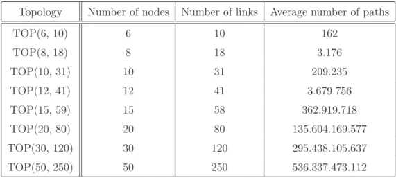
2.9 Evaluation . . . 35

2.9.1 Evaluation of The ILP Formulations . . . 37

2.9.2 Evaluation of The Heuristic Algorithms . . . 41

2.10 Conclusion . . . 44

3 Link-Level Anomaly Detection in Multi-Domain Networks 47 3.1 Introduction . . . 47

3.2 Problem Formulation . . . 49

CONTENTS

3.2.2 Problem Definition . . . 49

3.2.3 Architecture and Cost Model of Multi-Domain Anomaly Detection . 51 3.3 ILP formulation . . . 54

3.4 Heuristic Algorithm for Anomaly Detection in Multi-Domain Networks . . . 55

3.4.1 Computation of Candidate Monitoring Paths in Multi-Domain Net-works . . . 56

3.4.2 Greedy Monitor Location and Path Selection Algorithm . . . 56

3.5 Performance Evaluation . . . 58

3.5.1 Evaluation Methodology . . . 58

3.5.2 Numerical Results . . . 59

3.6 Conclusion . . . 65

III

Localization of Link-Level Network Anomalies

67

4.2 Network Model and Problem Statement . . . 71

4.3 Not all link pairs need to be distinguishable for localizing any single link-level anomaly . . . 72

4.4 Derivation of potential anomaly scenarios . . . 74

4.5 Anomaly localization cost . . . 77

4.6 ILP Formulation . . . 78

4.7 The Anomaly Localization Problem is N P-Hard . . . 80

4.8 Heuristic solution . . . 83

4.8.1 Monitor location selection . . . 83

4.8.2 Selection of localization paths . . . 84

4.8.3 Candidate path selection algorithm . . . 87

4.9.1 Comparing our Anomaly Localization Scheme with Existing Schemes 91

4.9.2 Evaluating the Scalability and Quality of the Heuristic . . . 95

4.10 Discussion . . . 99 4.11 Conclusion . . . 100

5 Conclusion and Perspectives 103

Appendix A 107 Appendix B 109 Appendix C 111 Appendix D 113 Appendix E 115 Bibliography 117 Acknowledgment 123

List of Figures

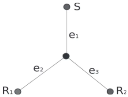
1.1 A tree-structured topology consisting of one source, one internal node and

two receivers . . . 5

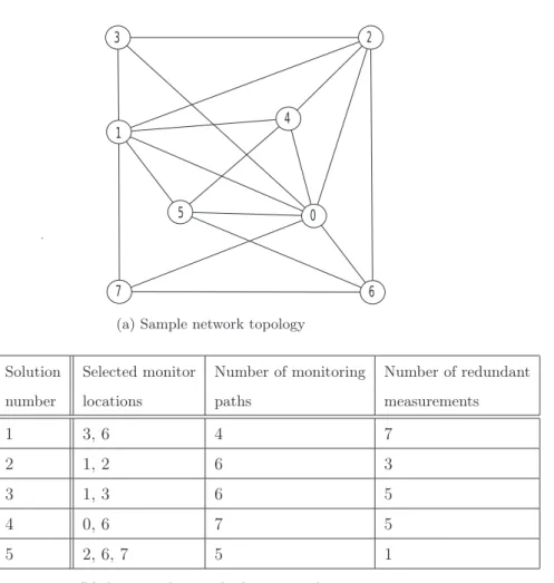
1.2 Example of a network topology . . . 8

1.3 Example of a detection infrastructure (gray nodes are monitor locations)

and detection paths (thick gray lines) . . . 9

1.4 Example of a single anomaly localization infrastructure and localization paths 9 1.5 Example of an anomaly detection solution with two monitors, three

detec-tion paths, and two redundant measurements . . . 12 1.6 Example of an anomaly detection solution with four monitors, seven

detec-tion paths, and zero redundant measurements . . . 12 1.7 Example of an anomaly detection solution with four monitors, seven

detec-tion paths, and two redundant measurements . . . 13 2.1 Illustrative example of anomaly detection solutions . . . 22 2.2 Example of a graph constructed out of a facility location instance with three

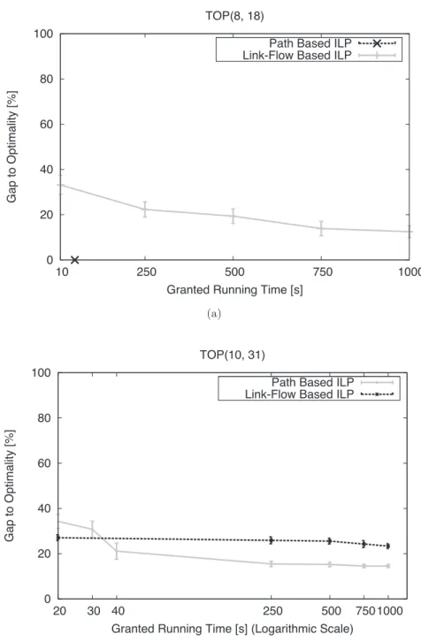
facility locations and four clients . . . 28 2.3 Gap-to-Optimality vs. Granted Running Time. (a) Results for the

topolo-gies with 8 nodes and 18 links; (b) Results for the topolotopolo-gies with 10 nodes and 31 links. . . 40 2.4 Performance results for our detection scheme with different values of α, β, and γ

(β = α); and for the existing detection scheme (denoted as EDS). (a) Results for topologies with 8 nodes and 18 links; (b) Results for topologies with 10 nodes and 31 links. . . 42

3.1 Per-domain detection solution . . . 50 3.2 Global detection solution . . . 50 3.3 Sample Multi-domain Monitoring Architecture . . . 52 3.4 Illustrative multi-domain network . . . 55 3.5 Sample multi-domain topology . . . 59

3.6 Monitoring cost: default setting . . . 60 3.7 Monitoring Cost: doubling inter-domain links . . . 61 3.8 CPU Running Time (s) . . . 62 3.9 Distribution of network links by path length groups . . . 63

3.10 Distribution of monitors and redundant measurements across domains . . . 64

4.1 Illustrative network topology, (a), and an associated detection solution, (b). 75

4.2 Example of a graph constructed out of a facility location instance with four facility loca-tions and four clients. . . 81

4.3 Average number of monitoring paths per anomaly for TOP(8, 18). The first histogram to the left presents results for solutions computed using the hybrid localization scheme (HLS), and the other histograms present results for the solutions computed using our anomaly localization ILP with different values of α (β = 1). . . 93 4.4 Localization costs for TOP(8, 18) . . . 94

4.5 Localization cost of the heuristic solutions, α >> β . . . 97

4.6 Impact of the number and the quality of candidate monitoring paths on the quality of the localization solution. RProc means random procedure (numerical results for TOP(15, 59)) 98

List of Tables

2.1 Notations used in the pseudo-codes . . . 31 2.2 Summary of the topologies considered in the evaluation . . . 37 2.3 CPU Running Time (CPU) and Gap-To-Optimality (GTO) for TOP(6,10)

and TOP(12,41). . . 39 2.4 CPU running time (OOM means Out Of Memory) . . . 41 2.5 Average number of deployed monitors + average number of redundant

mea-surements (network utilization) . . . 43 2.6 Resource utilization for SGA . . . 44 3.1 Notations used throughout this chapter . . . 53 4.1 Sets of suspect links for all potential anomalies . . . 76 4.2 Anomaly scenarios . . . 76 4.3 Summary of the topologies considered in the evaluation . . . 91 4.4 Average ILP computation time for TOP(8, 18) . . . 92 4.5 Heuristic computation time (all computations are done offline) and percentage of

List of Algorithms

1 Exhaustive greedy algorithm for anomaly detection . . . 32

2 Selective Greedy Algorithm . . . 34

- Procedure 1: candidatePathComputation(G, n1, n2, CL) . . . 36

3 Monitor location and path selection algorithm for anomaly detection in

multi-domain networks . . . 57

4 Monitor location and path selection algorithm for single anomaly localization 85

Glossary

CPU Central Processing Unit

EDS Existing Detection Solution

EGA Exhaustive Greedy Algorithm

GTO Gap To Optimality

HLS Hybrid Localization Scheme

ILP Integer Linear Programm

LP Linear Programm

NOC Network Operations Center

Part I

Background and Technological

Context

CHAPTER

1

Introduction

The Internet has experienced a transition from being a simple data transmission net-work serving a few users to becoming a multi-service netnet-work that supports various mul-timedia applications with high QoS requirements (e.g., loss rate, end-to-end delay, jitter, throughput, etc.) and serves a sharply growing number of demanding users. This is due to the rapid development of more and more powerful and affordable network devices (e.g., high-capacity transmission mediums, high-speed switching, high-capacity storage devices, etc.). The need for efficient network monitoring tools that ensure a desired network per-formance and provide QoS guarantees has subsequently increased. A large number of monitoring schemes and network measurement tools have been proposed in the literature. The simplest monitoring schemes make use of existing networking tools such as ping and traceroute [18][23]. They are qualified as simple because they do not require any spe-cific feature in the network. However their application is limited to detect and localize infrastructure failures and path outage [27]. Schemes that provide more detailed perfor-mance information have been proposed. They can be broadly divided into two categories, individual monitoring schemes (e.g., SNMP(Simple Network Management Protocol)-based schemes [7], RMON [28], Netflow [8]), and end-to-end monitoring schemes (e.g., [14] [24] [26] [9] [10] [11] [17] [16] [15][21] [20] [19] [29] [1] [6] [22] [2]). The basic idea of individual monitoring schemes is to equip every network device with a monitoring agent that collects performance statistics for the device and its incident links by snooping on the network traffic crossing it. Individual statistics are exported to a network operations center for analysis. The major problems of these schemes is that the monitoring infrastructure cost can be very high in large-size network, and the exportation of individual statistics to the operations center may generate a heavy burden on the network. End-to-end monitoring is an intuitive solution to these problems. The idea is to infer internal network performance through end-to-end measurements, which should require much less monitoring devices to be deployed in the network and minimize the monitoring overhead.

There exists another classification of monitoring schemes: passive monitoring schemes and active monitoring schemes. Passive monitoring infers the network performance by snooping on existing network traffic. There are two approaches to perform passive moni-toring:

– Two-point monitoring: this monitoring approach deploys two monitoring devices at the ingress and egress nodes of each monitored flow. Performance metrics are inferred by comparing measurements performed at ingress and egress monitors. This requires the timestamps of the monitors to be synchronized and all packets traversing them to be identified. However, the identification process might lead to serious scalability issues when the volume of traffic traversing the monitors is important.

– One-point monitoring: This monitoring approach requires one single monitor for monitoring one flow. It uses TCP acknowledgments to infer performance metrics between the point where the monitor is deployed and the sink of the monitored TCP flow (e.g., loss rate and round trip time on the segment between the monitor location and the sink of the monitored flow). Clearly, the application of this approach is restricted to TCP flows.

Active monitoring infers the performance of the network (e.g., availability, loss rate, delay, etc.) by making measurements on active monitoring flows, called in this context active probes, injected in the network to simulate existing network flows. The main dif-ficulty of active monitoring is to make active probes experience the same conditions as real traffic flows in order to achieve accurate measurements, without interfering with the network services.

Although the two monitoring approaches have their own drawbacks, the active moni-toring have two important advantages over passive monimoni-toring. the first is that it preserves privacy and confidentiality of services crossing the network since it does not make mea-surements on real traffic flows. The second is that it is possible using active monitoring to make measurements when there are no flows traversing the network. For instance, a ser-vice provider might need to check the availability and the characteristics of a network path previously not used before it transmits services on it, which is not feasible using passive monitoring.

Both active and passive end-to-end monitoring problems have been widely studied in the literature. Despite their divergence in terms of measured metrics and the approach of measurement acquisition, all the proposed schemes share a common important objective: guarantee a desirable network performance while minimizing the monitoring expense in

1.1. OVERVIEW OF END-TO-END MONITORING TECHNIQUES

terms of infrastructure cost and monitoring overhead. The aim of this thesis is to come up with an end-to-end network monitoring scheme that achieves this objective.

The remainder of this chapter is organized as follows. Section 1.1 provides a classifica-tion of existing end-to-end monitoring techniques. Secclassifica-tion 1.2 and secclassifica-tion 1.3 define the problem of link-level anomaly detection and link-level anomaly localization, respectively. Section 1.4 and section 1.5 describe the infrastructure requirements and the costs incurred for link-level anomaly detection and localization. section 1.6 and section 1.7 presents exist-ing link-level anomaly detection and localization schemes and their limitations, respectively.

1.1

Overview of End-to-End Monitoring Techniques

End-to-end monitoring techniques can be broadly classified into two categories: ana-logue and binary [22].

1.1.1

Analogue Monitoring

Motivated by the effectiveness of multicast communications in terms of bandwidth saving, the early end-to-end monitoring schemes used end-to-end active multicast probes to infer link-level loss rate, delay distribution, and bottleneck bandwidths (e.g., [3] [14] [26] [24] [4] [25]). The key idea is to correlate the copies of multicast probe packets ob-served at the multicast receivers to infer the performance of links within the multicast tree.

Figure 1.1: A tree-structured topology consisting of one source, one internal node and two receivers

Consider the logical multicast tree depicted in Figure 1.1 to illustrate. The loss events

are inferred as follows. If a copy of a multicast probe packet is received by R1 but not

the probe packet, then losses have likely occurred either on e1, or on e2 and on e3. A

probabilistic analysis of repeated multicast probes provides an estimation of the loss rates of the tree links with high probability (textite.g., [14]). Similarly, a probabilistic analysis of the correlations between the delays that make the copies of a probe packet issued by the multicast source to reach the multicast receivers provides an estimation of the link delay distributions (textite.g., [24]). Bottleneck bandwidths can be estimated through correlations of loss statistics across the multicast receivers (textite.g.,[26]).

Despite its potential benefits, multicast-based schemes cannot not be widely applied because multicast is so far only modestly deployed. Several research works proposed to emulate multicast-based monitoring schemes using unicast measurements (e.g., [9], [10] [11], [17], [16], [5]). The idea is to send two closely time-spaced packets, referred to as back-to-back packet pairs, from one server to pairs of receivers whose paths back to the source share a set of common links. The back-to-back packets issued from the same source and having the same characteristics are very likely to experience the same performance on the shared links. This performance correlation is exploited, in the same way as for multicast-based schemes, to infer link-level performance parameters.

1.1.2

Binary Monitoring

A new feature has been widely adopted by the monitoring research community. It con-sists in identifying the deviations of the network performance from a given performance baseline rather than estimating link-level performance measurements. This feature resets on the assumption that link performance is separable, which implies that a path expe-riences bad performance if and only if at least one of its constituent links expeexpe-riences bad performance [15]. Thus, identifying link-level performance violations can be done by identifying paths that violate performance thresholds. More specifically, according to the property of separable performance, it is enough to monitor a set of paths that cover all links of the network for detecting all potential link-level performance violations. Further paths need to be monitored to localize the source(s) of the violation(s). [15] states numerous separable link performance parameters such as connectivity, high-low loss model and delay spike model.

Many research works exploited the property of separable performance to devise link-level anomaly detection and localization schemes (e.g., [21], [20], [19], [29], [1], [6]). we next investigate the problems of link-level anomaly detection and localization.

1.2. LINK-LEVEL ANOMALY DETECTION

1.2

Link-Level Anomaly Detection

The goal of link-level anomaly detection is to detect any performance degradation or infrastructure failure that would occur on the network links. In this thesis we consider separable anomalies that satisfy the separable performance property established in [15]. As mentioned previously, a path exhibits a separable anomaly if and only if at least one of its constituent links is anomalous. The trivial conclusion that can be drawn from this property is that for detecting all potential link-level anomalies in a given network, a set of paths that cover all links of the network must be monitored. A link is said to be covered if it is traversed by at least one monitored path. It can be easily shown that this is a necessary and sufficient condition for link-level anomaly detection.

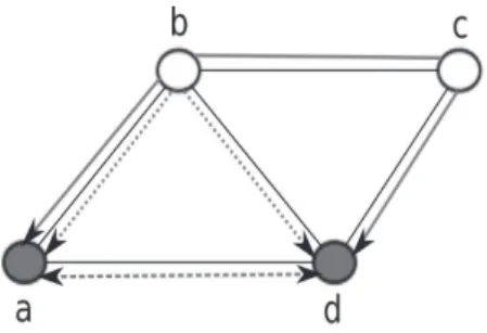
The information delivered by the anomaly detection process is a set of anomalous paths, i.e., monitored paths that exhibit an anomaly. We refer to the set of links that are traversed by only anomalous monitored paths as the set of suspect links. It cannot be decided whether these links are anomalous using only the detection information. Let us consider the network topology depicted in Figure 1.2 to illustrate. Suppose that nodes a and d are equipped with monitoring devices. Consider the bidirectional paths

p1 = &(a, b), (b, c), (c, d)', p2 = &(a, b), (b, d)' and p3 = &(a, d)' that cover all links

of the network (refer to Figure 1.3 for an illustration). Assume that the detection process

which monitors these three paths reports that p1is anomalous. According to the separable

performance property, all links that are traversed by paths not exhibiting the anomaly

are surely not anomalous. We conclude that all links that are not traversed by p1 as well

as the link connecting node a to node b are not anomalous. Thus, the set of suspect

links is {(b, c), (c, d)}. We say that paths p1, p2 and p3 cannot distinguish between

the links (b, c) and (c, d). Further paths must be monitored in order to decide whether (b, c), (c, d) or both links are anomalous. This operation is called link-level anomaly localization.

1.3

Link-Level Anomaly Localization

Link-level anomaly localization aims at identifying the root cause of a detected anomaly. Let us consider again the anomaly scenario described in the previous section. The set

of suspect links constructed out of the detection information when path p1 exhibits an

Figure 1.2: Example of a network topology

two additional paths must be monitored. Either path must traverse one of the two suspect links, but not both. Additional monitoring devices may need to be deployed. In this case, one additional monitoring device need to be deployed on node c. The paths monitored

during the localization process are p4 = &(a, b), (b, c)' and p5 = &(c, d)'. If both paths

exhibit an anomaly, then both suspect links are anomalous. Otherwise the suspect link traversed by the path that exhibits an anomaly is anomalous.

A sufficient condition for localizing link-level anomalies has been been established in the literature (e.g., [21], [6], [1]). It consists in deploying a set of monitoring devices that can distinguish between every two subsets of the network links. This implies that for each pair of link subsets there exists a path between the deployed monitoring devices whose intersection with exactly one of the two subsets is not empty. For instance, for the sample

topology depicted in Figure 1.2, there is only one path, p6 = &(a, b)', that can distinguish

between the subsets {(a, b), (b, c), (c, d)} and {(b, c), (c, d)}. Thus, monitoring devices must inevitably be deployed on node a and node b. In practice, multiple link-level anomalies that involve a large number of links are rare events. Therefore, numerous works bound the number of concurrent anomalies in an attempt to minimize the localization cost, e.g., [1] claims that anomalies involving more than three links are very unlikely to occur.

1.4

Infrastructure Requirements for Link-Level Anomaly

De-tection and Localization

The anomaly detection (respectively localization) infrastructure consists of a set of monitoring devices placed at a subset of the network nodes such that there exists a set of paths between the nodes equipped with monitoring devices that covers all links of the network (respectively distinguish between all subsets of the network links pairwise). The

1.4. INFRASTRUCTURE REQUIREMENTS FOR LINK-LEVEL ANOMALY DETECTION AND LOCALIZATION

network nodes that support monitoring devices are referred to as monitor locations. The term monitoring path is used interchangeably with the term detection paths to designate paths that are monitored for anomaly detection, and is used interchangeably with the term localization paths to designate paths that are monitored for anomaly localization.

Figure 1.3 shows an example of a detection infrastructure and detection paths for the sample network topology depicted in Fig 1.2, and Figure 1.4 shows an example of a single link-level localization infrastructure, i.e., simultaneous anomalies involving multiple links are not considered, and localization paths for the same network topology.

Figure 1.3: Example of a detection infrastructure (gray nodes are monitor locations) and detection paths (thick gray lines)

Figure 1.4: Example of a single anomaly localization infrastructure and localization paths

Usually, the anomaly detection infrastructure is continuously active, whereas the anomaly localization infrastructure is activated only upon detecting an anomaly. For instance, if path &(a, b), (b, c), (c, d)' exhibits an anomaly, then, activating only the monitors on node a and node c and monitoring only the localization path &(a, b), (b, c)' is sufficient to pinpoint the anomalous link. The rationale behind activating the anomaly localization process only upon detecting an anomaly is that network anomalies are

typi-cally rare events. Moreover, depending on the network topology, running the localization process continuously may incur a heavy burden on the underlying network.

Furthermore, measurements collected by active monitoring devices are exported to a network operations center, referred to as NOC. The NOC analyzes and correlates the mea-surements collected individually by the monitoring devices. When it detects an anomaly, it triggers the anomaly localization process by activating some monitoring devices that can distinguish between the suspect links.

1.5

Link-Level Anomaly Detection and Localization Costs

The anomaly detection and localization costs consist of the following costs:

– Infrastructure cost: this is the effective cost of acquiring, deploying and maintaining software and hardware monitoring devices.

– Communication cost: this is the cost of communications between the NOC and the monitoring devices that are deployed in the network. The NOC collects monitoring measurements from the monitoring devices that are activated for anomaly detection periodically. When an anomaly is detected, the NOC triggers the localization phase by activating the localization process on a subset of the monitors deployed that can distinguish between the set of suspect links constructed out of the detection measurements. It is of great importance to choose the locations where to deploy monitors carefully, in order to reduce the communication overhead and delays. – Probe cost: this cost expresses the load of monitoring flows on the network.

Mea-surements of links that do not provide any extra detection/localization information is highly indesirable. Indeed, such measurements increase the detection/localization delays and overhead.

1.6

Monitor Location and Monitoring Path Selection for

Link-Level Anomaly Detection and Localization

One of the problems that received great interest within the research community on network monitoring is formulated as follows: How to choose monitor locations and how to select monitoring paths that can detect/localize all potential anomalies while minimizing the costs incurred and reducing the detection/localization delays (e.g., [6] [1] [20] [21] [29]).

1.7. LIMITATIONS OF THE EXISTING LINK-LEVEL ANOMALY DETECTION AND LOCALIZATION SCHEMES

Almost all existing network monitoring schemes apply a two-step approach for monitor location and monitoring path selection. Usually, the first step selects the smallest set of monitor locations that can detect/localize all potential anomalies. The second step selects the smallest set of paths between the monitor location selected at the first step that cover/distinguish between all potential anomalies (e.g., [6] [1]).

[21] applies an inverse two-step approach of monitor location and monitoring path se-lection for localizing multiple link failures. The first step selects a set of optimal monitoring paths that can localize all potential multiple failures, whereas the second step selects the smallest set of monitor locations that can monitor paths selected at the first step.

[29] proposes a multi-round link-level anomaly detection schemes. It takes into account the capacity of the network links to support monitoring flows and the capacity of monitoring devices to generate probe messages while selecting monitor locations. The result is a minimal set of monitor locations and monitoring paths that covers all the network links in a certain number of rounds.

As mentioned previously, it is agreed that monitoring a set of paths that covers all network links is necessary for detecting all potential link-level anomalies. However, the set of paths that is to be monitored to pinpoint the source of a detected anomaly has been defined in two ways. The first proposes to monitor a set of paths that can distinguish between every pair of link-level anomalies for any detected anomaly (e.g., [1]), whereas the second monitors a set of paths selected upon detecting an anomaly that can distinguish only between the set of suspect links (e.g., [2]).

Both the problems of monitor location and the problem of path selection are N P-Hard. Therefore, heuristic algorithms, most of them greedy, have been proposed.

1.7

Limitations of The Existing Link-Level Anomaly

Detec-tion and LocalizaDetec-tion Schemes

The existing anomaly detection and localization schemes present the following limita-tions:

– The optimization metrics usually considered for monitor location selection (minimiz-ing the number of monitors that are to be deployed) and monitor(minimiz-ing path selection (minimizing the number of paths that are to be monitored) do not reflect the mon-itoring costs properly. For instance, although minimizing the number of monmon-itoring

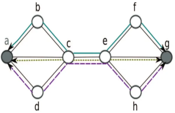
paths is highly desirable to reduce the communication overhead due to exporting the measurements carried out for each monitored path to the NOC at each time interval, this is likely to generate heavy probe overhead. For example, Figure 1.6 and Fig-ure 1.5, each depicting a different anomaly detection solution for the same network topology, illustrate that reducing the number of detection paths from seven paths to three paths generates redundant measurements.

Figure 1.5: Example of an anomaly detection solution with two monitors, three detection paths, and two redundant measurements

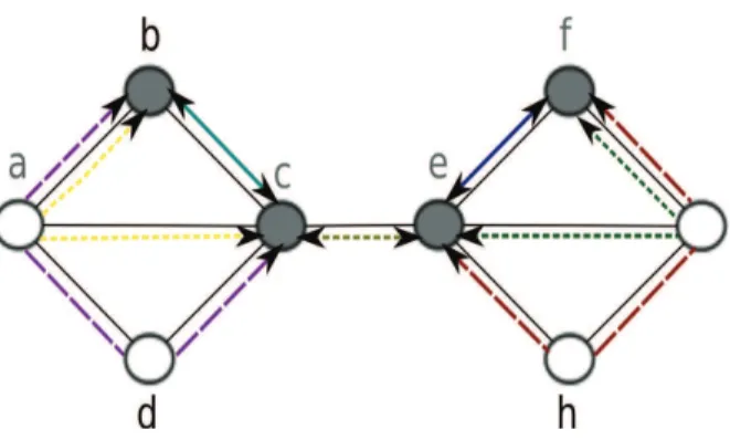
Figure 1.6: Example of an anomaly detection solution with four monitors, seven detection paths, and zero redundant measurements

– The step-wise approaches for monitor location and monitoring path selection ignore the interplay between the optimization objectives of each step, which may lead to sub-optimal consumption of the network resources. We contend that the number and locations of monitoring devices have an impact on the quality of monitoring paths. For instance, Figure 1.6 shows that two monitoring devices are sufficient to detect all potential link level anomalies of the considered network topology, however, as illustrated in Figure 1.5, at least four monitoring devices are required to cover

1.7. LIMITATIONS OF THE EXISTING LINK-LEVEL ANOMALY DETECTION AND LOCALIZATION SCHEMES

Figure 1.7: Example of an anomaly detection solution with four monitors, seven detection paths, and two redundant measurements

the network links without generating redundant measurements. Figure 1.7 shows that redundant measurements cannot be avoided when changing the locations of two among the four monitoring devices of the solution presented in Figure 1.5, which illustrates the correlation between the locations of monitoring devices and the quality of monitoring paths.

– The anomaly detection scheme proposed in [29] addresses the issues discussed above in that it takes into account the capacity of links to support monitoring flows while selecting monitor locations. However, the major limitation of the proposed scheme is that links are covered over multiple rounds, which increases the detection delays proportionally to the number of rounds.

– Selecting localization paths online, i.e., upon detecting an anomaly, as done in [2], induces non-negligible delay.

– Monitoring a set of localization path that distinguishes between every pair of link-level anomalies whenever an anomaly is detected, as done in [1], incurs unnecessary overhead and delay.

– Heuristic detection and localization algorithms select monitoring paths from a set of candidate paths. This latter is described in the literature as a small subset of the net-work paths. However, there is any indication on how such a set is computed. Clearly, reducing the number of candidate paths is fundamental for scalability, however, the reduction must be done in a measured way in order not to degrade the quality of the monitoring solution.

1.8

Contributions of The Thesis

The goal of this thesis is to come up with a cost-effective, fast and accurate monitoring scheme. The proposed scheme is to some extent similar to recent monitoring schemes in that it performs anomaly detection and localization in two phases. However, it overcomes the limitations raised in the previous chapter. The main contributions can be summarized as follows.

– The optimization objectives considered for monitor location and monitoring path selection are not limited to minimizing the number of monitoring devices that are to be deployed and the number of paths that are to be monitored. Rather, monitors are placed in a measured way such as the cost and the delays of communications with the NOC are minimized. Moreover, measurements that do not provide extra information are avoided, thereby reducing the monitoring overhead.

– Monitor locations and monitoring paths for anomaly detection, respectively for anomaly localization, are selected in one single step. It will be demonstrated that the joint selection achieves a good trade-off between the monitoring infrastructure cost and the monitoring overhead and delays.

– The condition on the set of paths that need to be monitored for localizing single link-level anomalies established in [1] is proved to be sufficient but not necessary. A necessary and sufficient condition is developed.

– A demonstration that full localization solutions, i.e., monitoring devices that are to be activated and paths that are to be monitored upon detecting a given single link-level anomaly, can be derived offline is provided.

– The anomaly detection and localization problems are formulated as ILPs. Both problems are shown to be N P-hard.

– Heuristic algorithms for anomaly detection and for anomaly localization are devised. Candidate monitoring paths are selected in a careful way, in order not to degrade the quality of the detection/localization solutions, while ensuring the scalability of the heuristic algorithms.

1.9. OUTLINE OF THE THESIS

– Operational constraints (e.g., limiting the capacity of monitoring devices to generate and manage monitoring flows, limiting the capacity of links to support monitor-ing flows, etc. ) can be easily introduced into the ILP formulations and the heuristics.

1.9

Outline of The Thesis

The remainder of the thesis is divided into two parts: Detection of Link-Level Net-work Anomalies and Localization of Link-Level NetNet-work Anomalies. The former part is composed of Chapter 2 and Chapter 3. The former chapter addresses the problem of link-level anomaly detection in mono-domain networks, whereas the latter chapter investigates the same problem in multi-domain networks. The latter part addresses the problem of link-level anomaly localization. It is composed of Chapter 4. Chapter 5 concludes the dissertation and presents future perspectives.

Part II

Detection of Link-Level Network

Anomalies

CHAPTER

2

Link-level Anomaly

Detection in

Mono-Domain Networks

2.1

Introduction

Most existing monitoring approaches operate in two phases (e.g., [2], [29], [1], [19], [2]). The first phase is the anomaly detection phase. It consists in deploying as few resources as possible such that all links of the network are covered in order to detect all potential link-level anomalies. The second phase is the anomaly localization phase. It is triggered upon detecting an anomaly in order to identify its root cause.

In this chapter, we focus on the anomaly detection phase. We revisit a widely studied problem that is the placement of monitoring devices and the selection of monitoring paths for anomaly detection (e.g., [29], [2], [1], [19], [6], [21], [32], [37], [34], [36], [35]). The moti-vation behind our work is that existing solutions suffer from two major shortcomings. The first is that most of them adopt a two-step approach for monitor location and monitoring path selection, and do not address the trade-off between the optimization objectives of each steps. The monitor location step selects locations for a minimal set of monitoring devices such that all links of the network are covered. The monitoring path selection step computes a minimal set of paths between the deployed monitors that cover all links of the network. The second is that existing monitoring cost models do not meet the requirements of the monitored networks. For instance, the number of monitoring paths does not reflect the effective monitoring load. Indeed, minimizing the number of monitoring paths is very likely to produce long monitoring paths that cover some network links multiple times, and thus, generating extra monitoring overhead and extending the detection delays. Further-more, the monitor locations should be selected carefully with regard to the NOC location