Magnetic properties of paramagnetic systems : density functional studies

Université de Montréal

Magnetic Properties of Paramagnetic Systems: Density functional Studies

par Seongho Moon

Département de Chimie faculté des Arts et des Sciences

Thèse présentée à la faculté des études supérieures en vue de l’obtention du grade de

Philosophiae Doctor (Ph. D) en Chimie

Mai 2003

, i-r

Université

de Montréal

Direction des bibliothèques

AVIS

L’auteur a autorisé l’Université de Montréal à reproduire et diffuser, en totalité ou en partie, par quelque moyen que ce soit et sur quelque support que ce soit, et exclusivement à des fins non lucratives d’enseignement et de recherche, des copies de ce mémoire ou de cette thèse.

L’auteur et les coauteurs le cas échéant conservent la propriété du droit d’auteur et des droits moraux qui protègent ce document. Ni la thèse ou le mémoire, ni des extraits substantiels de ce document, ne doivent être imprimés ou autrement reproduits sans l’autorisation de l’auteur.

Afin de se conformer à la Loi canadienne sur la protection des renseignements personnels, quelques formulaires secondaires, coordonnées ou signatures intégrées au texte ont pu être enlevés de ce document. Bien que cela ait pu affecter la pagination, il n’y a aucun contenu manquant.

NOTICE

The author of this thesis or dissertation has granted a nonexclusive license allowing Université de Montréal to reproduce and publish the document, in part or in whole, and in any format, solely for noncommercial educational and research purposes.

The author and co-authors if applicable retain copyright ownership and moral rights in this document. Neither the whole thesis or dissertation, nor substantial extracts from it, may be printed or otherwise reproduced without the author’s permission.

In compliance with the Canadian Privacy Act some supporting forms, contact information or signatures may have been removed from the document. While this may affect the document page count, t does not represent any loss of content from the document.

II

Université de Montréal Faculté des études supérieures

Cette thèse intitulée

Magnetic Properties of Paramagnetic Systems: Density Functional Studies

présentée par: Seongho Moon

a été évaluée par un jury composé des personnes suivantes:

Professeur Tucker Carrington, Président-rapporteur

Professeur Dennis R. Salahub, Directeur de recherche

Professeur Math jas Emzerhof, Membre du jury

Professeur VladimirG. Maikin, Examinateur externe _____________________

III

C

RESUME

Le propos principal de cette thèse est d’étudier les propriétés magnétiques des espèces paramagnétiques possédant des électrons non appariés. Cette étude a été réalisée à l’aide de la théorie de la fonctionnelle de la densité (DFT).

Afin de simuler correctement les paramètres de résonance magnétique, nous proposons une approche combinée mécanique quantique/mécanique moléculaire (QM/MM). La région quantique est tronquée par des potentiels capuchons à un électron quantique (QCP) qui sont paramétrés de façon à reproduire les structures moléculaires comportant tous les électrons ainsi que les distributions de charge. Les effets de l’environnement sont modélisés en incluant le champ électrique, causé par le domaine MM, dans l’Hamiltonien DfT. Cette approche montre que les effets électrostatiques dus à la partie MM transfèrent principalement à la partie QM à travers les orbitales Kohn-Sham non soumises au champ et donc implicitement aux énergies correspondantes. Nous examinons plusieurs systèmes modèles partant de petites molécules organiques et allant jusqu’à des modèles biologiques. Grâce à la simplicité de l’implémentation, l’approche présentée ici nous permet d’étudier les paramètres magnétiques de modèles réalistes notamment des sites actifs biologiques.

Nous présentons une expression générale pour les déplacements RMN paramagnétiques qui est indépendante des paramètres empiriques et permet des applications de calculs. Pour un cas particulier (doublet Kramers spatialement non dégénéré) dans lequel il n’existe pas d’états excités accessibles thermiquement, l’équation exécutable pour les déplacements paramagnétiques est dérivée en utilisant un Harniltonien effectif de spin et la statistique de Boltzmann. Les déplacements chimiques RMN paramagnétiques sont décomposés en trois contributions dans notre équation: une contribution orbitalaire, une contribution de contact de fermi et enfin une contribution de pseudo-contact. Les contributions individuelles sont déterminées par les calculs ab initio des paramètres de résonance magnétique. Afin de valider ce travail, des calculs DFT ont été réalisés pour

(J

les déplacements chimiques RMN de certains complexes d’oxydes d’azote, de

C

Iv

protéine/cuivre bleu et d’irnidazole cyanidrique ferrique. Les études théoriques, comparées avec les travaux expérimentaux, fournissent trois indications principales : (1) l’approche présentée ici dans le cadre de la DFT donne des simulations fiables et prometteuses. (2) les déplacements orbitalaires sont facilement approxirnés par les déplacements chimiques RMN dans des environnements à couche fermée similaires. (3) les déplacements de contact de Fermi dominent le déplacement chimique total et sont très sensibles aux changements structurels.

Mots-clés: théorie de la fonctionnelle de la densité, QM/MM, QCP, Hamiltonien effectif de spin, déplacement orbitalaire, déplacement de contact de Fernii, déplacement de pseudo-contact, paramètres de résonance magnétique.

V

ABSTRACT

Ihe main concem ofthis thesis is to investigate the magnetic properties ofparamagnetic species which have unpaired electrons. The present study is based on density fttnctional theory (DFT).

In order to simulate magnetic resonance parameters efficiently, we propose a combined quantum mechanics/moÎecular mechanics (QM/MM) approach. The quantum region is truncated by one-electron quantum capping potentiais (QCPs) which are parameterized to duplicate ail-electron motecular structures and charge distributions. The effects from the surroundings are modeled by including the electric field, due to the MM domain, in the DFT Hamiitonian. This approach shows that the electrostatic effects from the MM part mainly transfer to the QM part irnplicitÏy through the fieid-free Kohn-Sham orbitais and through the corresponding energies. We examine severai mode! systems ranging from small organic moiecutes to bioiogical models. Because of the simplicity of the impiementation, the present approacli enables us to investigate the magnetic parameters of large, realistic modeis ofbioiogicai active sites.

For paramagnetic NMR shifis, we provide a general expression which is independent of empiricai parameters and give the recipe for practical calculations. For a special case (spatially non-degenerate Kramers doublet) with no thermaily accessible excited states, the working equation for the paramagnetic shifts is derived by using an effective spin Hamiltonian and Boltzmann statistics. The paramagnetic NMR shifts are decornposed into the three contributions within the equation: the orbital, Fermi contact, and pseudocontact contributions. The individuai contributions are determined by the first principles caiculations of the magnetic resonance parameters. For validation, the DFT calculations are carried out for the NMR chemical shifis ofsome nitroxides, blue copper proteins, and ferric cyanide-imidazoie complexes. The theoretical studies, compared with the experimentai works, indicate mainiy three things: (1) the present approach within the DFT framework provides reiiabie and promising simulations; (2) the orbitai shifts are readily approximated by the NMR chemical shifis in simitar, closed-sheli environments;

VI

(3) the Fermi contact shifis dominate the total shifis and they are very sensitive to structural changes.

Key words: Density functional theory, QM/MM, QCP, effective spin Hamiltonian, orbital shifi, Fermi contact shift, pseudocontact shift, magnetic resonance parameters.

VII

ACKNOWLEDGEMENTS

During my study, I have reaÏized that I am a really tiny existence in the vast ocean of science. Ï am sure that I would lose my way there without the guidance ofmy supervisor, Professor Dennis R. Salahub. I cannot but thank you for expanding my horizons in science and making me scientist. The driving force that I could overcome adversity in the days arose from the fact that I wanted to be your real student.

I would like to thank Dr. Serguei Patchkovskii for letting me understand the big picture and details of magnetic properties (speciaÏly, paramagnetic NMR theory). I cannot forget happy moments whlle doing science and sports together.

I am grateful to Dr. Gino DiLabio for providing carbon capping potentials and for ftuitftd discussions ofQM/MM theories.

I wish to acknowledge the present and past members of Salahub group, Mark, Steeve, Sébastian, Elisa, Deiphine and the present and past members of SIMS theory group, John, Dennis, Raphael, Hilaire, Sergei, Nelaine, Luciano, Gwang-Soo, Yoshii for your kind support and stimulating discussions.

VIII

o

For nq wsfe Ge Won and

my

daughter Yejin

Ix

TABLE 0F CONTENTS

Resume III Abstract _V Acknowledgements VII Dedication VIII Table of contents IX

List of tables _XII

List of figures XV

List of abbreviations _XVII

Introduction XIX

Cliapter 1. Theoretical Background _I

1.1 Electromagnetism

1.1.1. Units in Electrornagnetism

1.1 .2. Charged Particles in a Magnetic FieÏd; Minimal Coupling 3

1.2. Density Functional Theory 6

1.2.1. Kohn-Sham Approach $

1.2.2. Approximate Exchange-Corretation Functionals 11 1.2.2.1. Density Matrices and Pair Correlation Functions 11

1.2.2.2. Fermi and Coulomb Holes 14

1.2.2.3. Adiabatic Connection 16

1.2.2.4. Local Spin Density Approximation (LSDA) 18 1.2.2.5. Generalized Gradient Approximation (GGA) 20 1.2.2.6. meta-Generalized Gradient Approximation (meta-GGA) 22

1.2.2.7. Hybrid Functionals 22

1.2.2.8. Optimized Effective Potential (OEP) 23

1.3. Magnetic Resonance Pararneters 25

1.3.1. Perturbation Theory 29

X

1.3.3. Nuclear Spin-Spin Coupling Tensors ₄₀

1.3.4. Hyperfine Coupling Tensors ₄₂

1.3.5. EPR g-tensors ₄₃

1 .4. References ₄₆

Chapter 2. QM/MM Approach for Magnetic Properties ₅₀

2.1. Introduction ₅₀

2.2. Theory ₅₂

2.2.1. Quantum Capping Potentials (QCPs) 52

2.2.2. Kohn-Sham (KS) Electronic Energy in Quantum Capping Potentiats and

MM Electronic fields ₅₄

2.2.3. Electrostatic Contribution to Magnetic Resonance Parameters 55

2.2.3.1. NMR Chemical Shielding Tensors 56

2.2.3.2. Other Magnetic Resonance Parameters 61

2.3. Implementation and Computational Details 63

2.3.1. NMR Chemical Shietding Tensors and Spin-Spin Coupling Constants 63

2.3.2. Kyperfine Coupling Tensors 64

2.4. Results and Discussion 65

2.4.1. NMR Chemical Shielding Tensors 65

2.4.2. Nuclear Spin-Spin Coupling Constants 7$

2.4.3. Kyperfine Coupling Tensors $0

2.5. Conclusion _$9

2.6. References ₉₁

Chapter 3. ParamagnetïcNMR Shifts 94

3.1. Introduction ₉₄

3.2. Short Theoretical Reviews of Pararnagnetic Systems 96

3.3. Paramagnetic Shifis for the General Case 101

3.4. Paramagnetic Shifts for an Isolated Krarners Doublet State 105

3.5. Implementation and Computational Details 113

XI

3.5.2. Blue Copper Proteins 116

3.5.3. Ferric Cyanide-lmidazole Complexes of Heme Proteins 118

3.6. Resuits and Discussion 120

3.6.1. Nitroxides 120

3.6.2. Blue Copper Proteins 131

3.6.3. Ferric Cyanide-Imidazole Complexes of Heme Proteins 138

3.7. Conclusion 141

3.8. References 143

Global Conclusions and Perspectives 147

XII

LIST 0F TABLES

Table 1.1. Conversions of some units and expressions between MKS-Sl and Gaussian

cgs Systems. 3

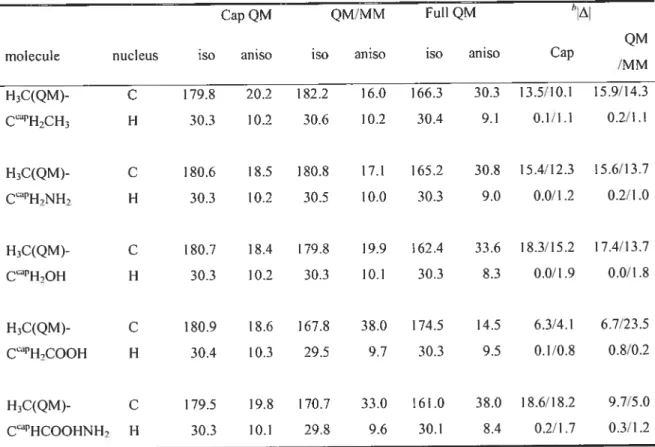
Table 2.1. Calculated NMR chemical shielding constants (in ppm) using quantum capping potentials (QCPs) for small organic molecutes in comparison with full QM

resuits. 67

Table 2.2. Calculated NMR chemical shielding constants (in ppm) using QCPs for propanoic acid and alanine in comparison with full QM results. 69

Table 2.3. Calculated NMR chernical shielding constants (in ppm) for some organic

molecules. ₇₀

Table 2.4. Calculated NMR chemical shielding constants (in ppm) for neutral histidine. 73 Table 2.5. Calculated NMR chemical shielding constants (in ppm) for the base of

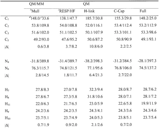
cytosine monophosphate (CMP). 77

Table 2.6. Calculated nuclear spin-spin coupling constants (in Hz) for the base of

cytosine monophosphate (CMP). 79

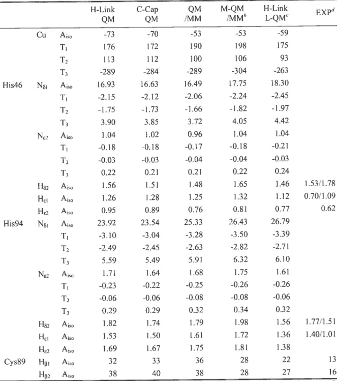
Table 2.7. Calculated hyperfine parameters ofazurin in MHz. 84

Table 2.8. Calculated hyperfine parameters ofstellacyanin in MHz 25

Table 2.9. Comparison of Mulliken spin populations for azurin and steÏlacyanin models, with different approaches for the dangling bond capping. $6

XIII

Table 3.L CaÏculated isotropic ‘H NMR chernical shifis (in ppm) ofa series ofaromatic

t-butyl nitroxide radicals at295 K. 121

Table 3.2. Calculated electronic g-tensors of a series of aromatic t-butyl nitroxide

radicals. 122

Table 3.3. Calculated Fermi contact (isotropic hyperfine) coupling constants (in MHz) of

a series ofarornatic t-butyl nitroxide radicals. 123

Table 3.4. Calculated fermi contact (isotropic hyperfine) coupling constants (in MHz) of 2-methylphenyl-t-butylnitroxide radical according to the angle . 124

Table 3.5. Calculated isotropic ‘3C NMR chemical shifts (in ppm) ofa series ofaliphatic

nitroxide radicals at 298 K. 12$

Table 3.6. Calculated ‘5N and contact shifis (in pprn) and g-tensors of a series of

aliphatic nitroxide radicals at 29$ K. 129

Table 3.7. Calculated Fermi contact (isotropic hyperfine) coupling constants (in MHz) of

a series of aliphatic nitroxide radicals. 130

Table 3.8. Calculated ‘H NMR chemical shiifs (in pprn) ofthe histidines in blue copper

protein models. 132

Table 3.9. Calculated hyperfine structures (in MHz) ofhistidine hydrogens in blue copper protein models.

134

Table 3.10. Calculated hyperfine structures (in MHz) of selected heavy atoms in blue copper protein models.

xlv

0

_{Table 3.11. Calculated g-tensors ofblue copperprotein models. 137}

Table 3.12. CalcuÏated ‘3CN NMR chernical shifts (in ppm) in cyanide-bound prophyrin

complexes (S1/2) at 296 K. 139

Table 3.13. Calculated g-values of cyanide-bound prophyrin complexes (Sl/2) and

calculated hyperfine structures oftheir cyanide carbons. 140

Table 3.14 Calculated fermi coupÏing constants (in MHz) of selected nuclei of four

different cyanide-imidazole complexes ofiron (III). 140

xv

LIST 0F FIGURES

Figure 2.1. Schematic description of the partition into QM and MM regions using one electron quantum capping potentials.

53

Figure 2.2. The % errors of shielding constants with capping potentials vs. the number of

bonds from the capping carbon. ₆₈

Figure 2.3. Optirnized structure and numbering scherne for neutral histidine. 72

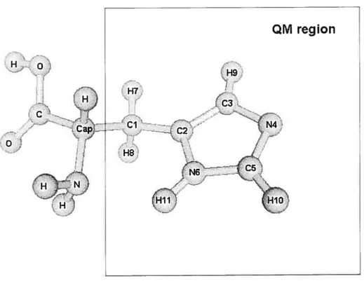
Figure 2.4. Optimized structure and numbering scheme of cytosine monophosphate

(CMP). 76

Figure 2.5. The QM part in wild type azurin from Pseudomonas aeruginosa; terminal carbon atoms were replaced by capping carbon atoms in the QM/MM calculations. 87

Figure 2.6. The QM part in steÏlacyanin from Cucurnis sativus; terminal carbon atoms were replaced by capping carbon atoms in the QM/MM calcutations. 88

Figure 3.1. Molecular structures and numbering schemes for a series of aromatic t-butyl nitroxides. The angle denotes the ONC1C2 dihedral angle. 115

Figure 3.2. Molecular structures ofa series ofaliphatic nitroxide radicals. 115

Figure 3.3. X-ray structures ofthe oxidized blue copper protein models. 117

Figure 3.4. Schematic view of the calculated cyanide-imidazole complex models of the Ïow-spin iron porphyrin. Here, II cornes from sperum whaÏe myogÏobin (Mb), III from

C

xv’

human myoglobin (Kb) or horse heart cytochrorne c(Cyt-c), IV from horseradish

peroxidase (HRP). ₁₁₉

Figure 3.5. Structural dependence of the Fermi contact (isotropic hyperfine) coupling constants in 2-methylphenyl-t-butylnitroxide radicat by change of the angle . 125

Figure 3.6. Top and side view of the active sites of the blue copper proteins and the

selected geometrical pararneters. ₁₃₃

Figure 3.7. Numbering scheme of cyanide-imidazole complexes of iron (III). 141

XVII

LIST 0f ABBREVIATIONS

DfT Density Functional Theory

HK Hohenberg and Kohn

KS Kohn and Sham

XC Exchange-CorreÏation

LDA Local Density Apptoximation LSDA Local Spin Density Approximation GGA Generalized Gradient Approximation

PW$6 Perdew-Wang86

B88 Becke88

PW9 I Perdew-Wang9 1 LYP Lee, Yang, and Parr

OEP Optim ized Effective Potential Kil Krieger, Li, and lafrate

BP Breit-Pauli

UDFT Uncoupled Density Functional Theory FPT Finite Perturbation Theory

NMR Nuclear Magnetic Resonance EPR Electron Paramagnetic Resonance ESR Electron Spin Resonance

GIAO Gauge Including Atomic Orbital IGLO tndividuaÏ Gauge for Localized Orbital LMO Localized Molecutar Orbital

CO Canonical Orbital

SOS-DfPT Sum-Over-State Density Functional Perturbation Theory

FC Fermi Contact

QM/MM Quantum Mechanics/MoÏecular Mechanics QCP Quantum Capping Potential

LA Link Atom

XVIII

GHO Generalized Hybrid Orbital ECP Effective Core Potential

MO Molecular Orbital

CMP Cytosine MonoPhosphate deMon density-ftrnctional Montreal DZVP Double Zeta plus Polarization PDB Protein Data Bank

RESP Restrained ElectroStatic Potential PPDME ProtoPorphyriniX DiMethyl Ester

Mb Myoglobin

Hb Hernoglobin

Cyt-c Cytochrorne

HRP HorseRadish Peroxidase

revPBE revised Perdew, Burke, and Ernzerhof STO Slater Type Orbital

XIX

INTRODUCTION

Most fields of magnetic resonance parameters (e.g. NMR chemical shifts, nuclear

spin-spin coupling constants, ESR A-tensors and g-tensors) have already been conquered by flrst-princip les electronic structure methods [l-5]. Therefore, the thesis focuses on two major, retated subjects which are beyond the limit of the present methods. One is a combined quantum mechanics/molecular mechanics (QM/MM) approach which enables us to simulate the magnetic resonances ofmacromolecuÏes including proteins and nucleic acids. The other is NMR chemical shifts of paramagnetic species (open-sheli systems) which have flot been exp Ïored properly yet by flrst-princip les methods.

Despite remarkable progress in computational chemistry in recent years, first-principles calculations for the magnetic resonance parameters of large biological and chemical systems are stiil far from routine. However, since most magnetic properties are local, we can divide the large system into the small reactive parts which are treated by high level quantum mechanics (QM) and the bulk which is treated by molecular mechanics (MM). This hybrid method bas two intrinsic problems: (1) how to partition the system into the QM and MM regions; (2) how to treat interactions between two regions. Here, we propose a QM/MM method to overcome the problems and to keep the balance between accuracy and expediency for evaluation of the magnetic resonance parameters of large systems such as proteins and nucleic acids. In the present approach, the frontier bonds between QM and MM regions are capped by one-electron quantum capping potentials (QCPs) which are parameterized to mimic the electronic character of a methyt group at the QM/MM boundary [6]. The advantages of this approach is that QCPs can be incorporated in most DfT programs with minimal code modification since they follow the format and concept of conventionat effective core potentials (ECP) [7]. Furthermore, some artificial effects of the link atom methods [8] and the special basis set manipulations ofthe localized self-consistent field (LSCF) [9] and the generalized hybrid orbital (GHO) [10] methods can be avoided and the number of electrons in the QM boundary can be reduced greatly compared to with the pseudobond approach [11]. In this approach, the QM parts are influenced by the the electrostatic effect of the environment

xx

represented by MM partial atomic charges. This description appears to be adequate in calculation of magnetic resonance parameters, as long as the MM part is not directly connected to the magnetic nuclei, and polarization effects of the QM part by MM partial charges dorninate interactions between the QM and MM subsystems.

The importance of nuclear magnetic resonance (NMR) spectroscopy for studies of paramagnetic species (open-sheli system), particularly in biomolecules, cannot be overestimated [12-14]. Paramagnetic NMR spectra serve as the source of tong-range structural data [15-17] and provide a sensitive probe of the magnitudes and signs of the spin density distributions [18,19]. Unique features of paramagnetic spectra are represented by spectral line broadening and a huge expansion of the chemical shifi scale. These resuit from the fact that the magnetic nuclei of paramagnetic species are strongly influenced by local magnetic fields arising from unpaired electrons. For the proper interpretation of the spectra, theoretical studies, which can give the direct relationship between the spectra and molecular and electronic structures, should be accompanied by experiments. So far, many theoretical approaches have been carried out to investigate the spectra [19-23]. However, frankly speaking, they are not pure theoretical approaches because they strongly depend on empirical parameters. Recent dramatic progress in the first-principles calculation ofmagnetic resonance parameters finally gives us a possibility to predict the spectra without any help of empirical factors. Hence, in the thesis, in order to achieve the goal, first, we derive a complete, general expression for the paramagnetic NMR shielding and give the recipe for practical calculations and, second, for a special case (spatially non-degenerate Kramers doublet) with no thenrialty poputated excited states, the working formalisms for the paramagnetic shift are derived by using an effective spin Hamiltonian and Boltzmann statistics.

The rest of thesis is organized as follows: In Chapter 1, we provide a short review of the unit systems and general theories for electrornagnetism. The general features of DFT are also explained, especially for exchange-correÏation functionals, since this work is based on the DfT method. f ina)ly, the theories and equations of various magnetic resonance

C

parameters (such as NMR chemical shielding tensors, nuclear spin-spin coupling tensors,

xx’

electron-nuclear hyperfine tensors, and EPR g-tensors) are reviewed. We focus on the non-relativistic, one-component case, where magnetic parameters are treated as second order properties, for practical reasons. In Chapter 2, we provide basic theories about QCPs and demonstrate how QCPs and MM charges can be handled in Kohn-Sham (KS) equations and how magnetic parameters are affected by them and this approach is appÏied to the magnetic pararneter calculation for several mode! systems. In Chapter 3, we provide a complete, general expression for the paramagnetic chemical shifts using the Boltzrnann statistics and derive working equations, which purely depend on the first principles calculations, for an isolated Kramers doublet state. This approach is applied to the chemical shifi caïculations of several organic radicaïs and metafloprotein models. FinaÏly in last chapter, some global conclusions are presented and possible future works are discussed.

o

XXII References

1. Helgaker, T., Jaszudski M., Ruud, K., CÏie,n. Rev. 1999, 99, 293.

2. Malkin, V. G., Maikina, O. L., Erisson, L. A., Salahub, D. R., In i’vlodern Densitv Functional Theorj’: A Tool /or ChemLrtn’; TÏieoreticaÏ anci C’omputationaÏ

Chemistiy; Seminario, J. M., Politzer, P., EUs.; Elsevier, Amsterdam, 1995. 3. Malkina, O. L, Vaara, J., Schirnmelpfennig, B., Munzarovâ, M., Maikin, V. G.,

Kaupp, M.,]. Am. Chem. Soc. 2000, 122, 9206.

4. Schreckenbach, G., Ph. D. Thesis, The University ofCalgary, Canada, 1996. 5. Lenthe, E. van; Wormer, P. E. S.; Avoird, A. van der I Chem. Phys. 1997, 107,

248$.

6. DiLabio, G. A.; Hurley, M. M.; Christiansen, P. A. J. Chem. Phys. 2002, 116, 957$.

7. ta) Christiansen, P. A.; Lee, Y. S.; Pitzer, K. S.]. Chem. Phvs. 1979, 71, 4445. (b) Christiansen, P. A.; Ermier, W. C.; Pitzer, K. S. Ann. Rev. Phvs. Chem. 1985, 36, 407. (c) Berger, A.; Dolg, M.; Kdchle, W.; StoIl, 14.; Preuss, K. Mol. Plnw. 1993, 80, 1431.

8. Singh, U.C.; Koliman, P.A.]. Comput. Chem. 1986, 7, 718. 9. Assfeld, X.; Rivai!, J.-L. Clie,,i. Phys. Lett. 1996, 263, 100.

10. Gao, J.;Amara, P.; Aihambra, C.; field, M. J.]. Phys. Chem. A 1998, 102, 4714. 11. Zhang, Y.; Lee, T.-S.; Yang, W. I Chem. Phys. 1998, 110, 46.

12. Bertini, 1.; Luchinat, C., NMR of Paramagnetic liolecules in Biological Systems, Benjamin/Cummings, Menlo Park, CA, 1986.

13. Bertini, 1.; Turano, P.; Vila, A. J., C’hem. Rev. 1996, 93, 2833.

14. Bertini, î; Luchinat, C.; Parigi, G., Solution NMR of Paiwnagnetic Molecules, Elsevier, Amsterdam, 2001.

15. Bertini, 1.; Luchinat, C.; Piccoioli, MethodEnzv,nol. 2001, 339, 314.

16. Bertini, I.; Luchinat, C.; Piccioli, M., Conceptsin Magn. Reson. 2002, 14, 259.

17. Allegrozzi, M.; Bertini, 1.; Choi, S.-N.; Lee, Y.-M, Luchinat, C, fur. ]. Inotg. Chem. 2002, 2121.

XXIII 18. Bei-tini, J., Luchinat, C., In PhysicaÏ Melhods:Jàr ChemLçt,ç, edited by Drago, R.

S., 2nd ed., HBJ, 1992, p. 500.

19. Lar Mar, G. N., Korrocks, ir., W. D., NMR of Paramagnetic MoÏecuÏes:

Principles andAppÏicafions, Academic Press, New York and London, 1973. 21. McGarvey, B. R., Coo,-d. Chem. Rev. 1998, 170, 75.

22. _{McGarvey, B. R.; Batista, N. C.; Bezerra, C. W. B.; Schultz, M. S.; Franco, D.}

W., Inorg. Chem. 1998, 37, 2865.

Chapter 1. Theoretical Background

1.1. Electromagnetism

1.1.1. Units in Electromagnetism

Prior to exploring magnetic properties in quantum rnechanics, the system ofunits should be mentioned. In spite of the attempted standardization to the MKS-SI system of units, the cgs-Gaussian system of units is often used in electromagnetism [1]. Conversions between the two systems may not be achieved easily because of the different definition for the electric charge q. Electromagnetic units are based on two relationships; Coulornb’s law for the electric charge and the law of Biot and Savart for the electric current.

Coulomb’slaw (electrostatic system)

MKS cgs Gaussian-cgs

f I f-JiJL f_9JL

4r) f t

where q is electric charge and r _{is the distance between charges. The constant Lo is the}

permittivity ofthe vacuum and has the value of 107”47cc2 C2/Nm2.

The Iaw ofBiot and Savart (electromagnetic system)

MKS cgs Gaussian-cgs

f P1 f =2L f =2--L

Chapter1. Theoretical Background 2

which relates the force F per length L between long, parallel conductors to the currents

i, and /, at the distance r. The constant p0 is the perrneability of the vacuurn and has the value of4tX iO N/A2.

In the MKS system the unit of electric charge is the Coulomb (C) which is defined from Ampere’s law (IC lAls) not from Coulomb’s law. Since the unit ofelectric charge is decided, the constants é0 and p() are fixed by the related laws.

In the cgs system there is no fundarnental unit of electric charge q. By Coulomb’s law the unit ofelectric charge q may be measured in dyne’ 2cm. The unit ofthe electric field

E is given in dyne’ 2/cm by the relationship F qE, and the electric potential V is dyne’ 2 by the relationship E = VV. However, the square of the potential V2 is clearly not force (dyne). This means that the units can flot show how rnany factors of the charge occur in a given equation. This defect can be rernoved by the consistent use of the unit ‘esu’ although it is not fundamental like the unit ‘Coulomb’ in the MKS system. Once the unit ‘esu’ is introduced, the unit of electric fleld E is dyne/esu and that of electric potential V is esulcm _(‘ erg/esu statvolt). The magnetic field B has its own unit ‘Gauss’ rather than dyne’ 2Icrn. This serves the same purpose as the introduction of the unit ‘esu’ on the electric side. In the cgs system the unit of electric current is abampere and this is not equal to statampere

₍

esulsec). Therefore the relationship between the two units must be determined. By experiment or by theory relating it to other fundarnental constants ‘abampere’ is equal to ‘statampc’ (where c is the velocity of light). The Gaussian-CGS system uses statampere and hence the constant c is included explicitly. The ftrndamental equations are readily reduced to dimensionless form.

In quantum mechanics, the Gaussian units are ofien combined with the atomic units where h (Planck’s constant divided by 2it), m (electronic mass) and e (electronic charge) are ail numerically unity. By the definition, the units of energy and length are redeflned as “Kartre&’ (E0 4.359$ x 1J’ erg) and “Bohr” (ao 5.291$ X 1O cm), repectively. Since in the Gaussian system electromagnetic units depend on mechanical units, they are

Chapter1. TI,et)retieal Background 3

also redefined as: (1) electronic charge (e force1 2/distance (Eo/ao)1 4.80325 X 10’° esu) (2) electric field (e/a02 1.715272 x i07 esu/cm2) (3) magnetic field (e/ao2c = 2.350540 x i09 G).

Table 1 .1 Conversions of some units and expressions between MKS-SI and Guassian-cgs Systems.

Quantity MKS-SI Gaussian-cgs

Distance Meter 102 cm

force Newton I

«

dyne

Energy Joule i07 erg

Charge Coulomb 2.998x109 esu

Current Ampere 2.998x1 statarnpere(esu/sec)

Electric Potential Volt 11299.8 statvolt Electric f ield Volt/meter 1/29980 statvoltlcm

Magnetïc field Tesla I gauss

4t/c2

47tEo 1

B B/c

1.1.2. Charged Particles in a Magnetic Field ; Minimal Coupling [2]

The electric field f and the magnetic field B are governed by Maxwell’s equations. The explicit forms ofthe equations are given by:

(in the MKS-SI system)

VB=0 VxB=p0E0+p0j (I.la)

VxE=——— (l.lb)

Chapter 1. Theoreticat Background 4

(In the Gaussian-cgs system)

VB=O VxB=.+i (l.2a)

ct e

VE=4irp VxE=L (l.2b)

e 3t

where p0 is the permeability of free space, E is the permittivity of free space, p is the charge density and

j

is the current density. The first terms ofEqs. (l.la, L2a) show that ail magnetic field unes which enter a particular closed surface must eventually leave the surface; thus there are no magnetic monopoles or sources of ‘magnetic charge’. The second terms of Eqs. (L la, 1.2a) show that a time-varying electric field and a current density generate a magnetic field. The first terms of Eqs. (1.lb and 1 .2b) indicate that the

amount of total electric flux through a given closed surface is proportional to the arnount of electric charge in the volume contained by that surface. The second terms of Eqs. (1.lb, 1.2b) indicate that a magnetic field changing in time acts as a source for a eÏectric field.

A scalar potnetial

_Ø

and a vector potential A can be introduced in terrns of the fields E and B (in the Gaussian system):

B=VxA (1.3)

e

An electron (negatively charged particle) at a position r in the fields E and B will experience a force (the Lorentz force)

F

= _e[E(r)+xB(r)1 =_e[_ _VØ(r)+!b<(VxA(r))1

= -VU (1.4)

Chapter 1. Theoreticat Background

O

The generalized potential U in the fields E and B can be obtained from the eq (1.4):

U=(é•A)+eç (1.5)

The Lagrangian is

L=T_U=±mé2_é _{.A—eØ (1.6)}

2 c

and the momentum becomes

3L e

p=—=mr——A (1.7)

e

Finally, the Hamiltonian is given by:

HZE .p—L

=±

mé2+eØ=_J_(p+A)2 +eØ (1.8a)

2 2m e

If atomic units are introduced, the Hamiltonian can be expressed as:

H=!(p+aA)2+Ø _(1.$b)

where a(= 1 / e) is the fine structure constant.

f rom now on, the atomic units based on the Gaussian system are employed in ail equations. Ail systems concemed here are time-independent.

Chapter 1. TÏieoretical Backgmuncl 6

•

1.2.

Density Functional Theory

In quantum mechanics, the conventional wave function based methods are very complicated to be used because the wave function cannot be probed experimentally and depends on 4N variables, three spatial and one spin variables for each of the N electrons. In fact, they cannot handle the interesting systems in biology and material science, which contain many atoms and electrons. The complexity can be diminished by repiacing the wave function and its associated Schrôdinger equation with the electron density and its associated calculational scheme since the electron density depends only on the three spatial variables (x, y, z) and that can be measured by X-ray diffraction.

The density functional theory (DFT)

_[31

uses the electron density as the main variable. The electron density is defined as

(1.9)

This function determines the probability of finding any of the N electrons within the volume element dr1 while the other N-1 electrons have arbitrary positions and spins in the state represented by ‘V. Electrons are indistinguishable and the probability of finding any electron at this position is, therefore, just N times the probability for one particular electron. The electron density is a positive function and goes to zero at infinity (r —>oo) and gives the total number of electrons when integrated over ail space,

p(r1)dr N (1.10)

In 1964, Hohenberg and Kohn justified theoretically the electron density as frmndamental quantity within quantum mechanics

_[41.

In their paper, they showed that a unique mapping between the ground state electron density and the external potential Vext exists based on the variational principle. This is the first Hohenberg-Kohn (HK) theorem. It implies that given a density, only one potential and wave function correspond to that

Chapter T TÏ,eoreticat Backgrouncl 7

density, so ail properties are functionals of the ground state density. This is indeed the case since any property may be determined as the expectation value of the corresponding operator and the wave function is determined by the density.

From now on, we will be concemed with systems of electrons moving in the field of fixed nuclei, so the external potential Vext is just the nuclear field. In this case, the

HarniÎtonian is

=

P

₊ + fr,f. (1.11)

—ZA

1=1 i=I A=1

I

rA 11

I

where A rnns over the M nuclei while j and

_j

denote the N electrons in the system. The operator

P

describes the kinetic energy ofthe electrons and the remaining two operators VNe and j2, represent the attractive electrostatic interaction between the nuclei and the electrons and the repulsive potential due to the electron-electron interaction, respectively. If the external potential VNe is taken for each density p(r) according to the first HK theorem, a functional E[pl yields the ground state energy of the system having this p as its ground state density. On the other hand, if a flxed extemal potential VNe is chosen, for which is the ground state and E0 the corresponding ground state energy, and we evaluate for each p(r) the expectation value of the Hamiltonian with the fixed VNe for

a functional E[p] will have Eo as Iower bound according to the variational principte

EJpJ=<PjpJ

P+Ç +Ç

_IIp]>

_{=Ttpj+VJpJ+SV\..p(r)drE)} (1.12)

This is usually refered to as the second HK theorem. It is cleary shown by the HK theorems that the electron density can replace the complicated wave function if one seeks

O

to catcutate the ground state energy. However, it shouÏd be noted that the 11K threoms are

Chapter 1. Theoretical Bac’kground 8

(D

only of importance from a theoretical point of view since the theorems are based on the exact functionals. In reaiity, we do flot know the exact functionals and the theorems do flot give any information about the unknown functionals. In 1965, Kohn and Sham

provided a creative and practicai way to soive many intrinsic probiems ofthe DFT [5].

1.2.1. Kohn-Sham Approach

In fact, so far, many pragmatic DfT models have been developed such as Thomas-fermi [61 and reiated models [3] that are based on the ideai uniform electron gas system and in which ail parts are expressed as pure functionais of the electron density. Unfortunateiy, it turns out that ail methods based on the Thornas-Fermi scheme are flot successfui in chemicai applications because it is hard to obtain the relationship between the spatial distribution ofthe eiectrons and their velocities which are needed for the kinetic energy.

In order to overcome the kinetic energy functional problem, Kohn and Sham introduced the orbital concept of a corresponding non-interacting system into DFT. In the Schrôdinger equation

(fJP

= F9’ : time-independent, non-reiativistic case) [7], the Hamiitonian is fixed and the wave function is the oniy variable. Hence, in the full interacting system, ail information on the interactions is in the wave function. The wave functions can be described by a linear combination of Siater determinants ‘-V.

‘=C19

(1.12)

In this system, the electron density and the kinetic energy can be represented using the naturai spin orbitais

_Ø1

which are the elements of the orthonormal set in which one electron density matrix (vide infra) is diagonal and their occupation numbers n1. The explicit forms are given by

Cliaptei 1. Theoretical Bcickgrotincl 9

O

p(r)=»1

IØj(r,s)12

(1.13)

and

T=n

<ØI_

V2

_Ø,>

(1.14)

On the other hand, in a non-interacting system, the Kamiltonian J-1 does flot have the electron-electron interaction terms and therefore the wave funtion P5 can be described by a single Slater determinant.

J=_iV+Zfr (1.15)

and

=

I

øi2

...ø I

(1.16)

In the Schrôdinger equation of the non-interacting system = EP), the external potential V (‘ E/,) can be adjusted in order to have the same ground state properties

(energy, density,...) as those of the full interacting system. In this system, the electron density and the kinetic energy can be represented by

p(r)=I(r)l2 (1.17)

Chapter1. Theoretical Backgrozind 10

T=<Ø1I_V2IØ> (1.18)

The N iowest eigenstates ç are determined by the self-consistent solution of the one electron Kohn-Sham equation which is derived by the variationai search for the minimum of the energy functional

EtpI

in the space of orbitais with the constraint of orthonomial orbitais. The Kohn-Sharn (KS) orbital equation can be obtained,

=

=ȯ

(1.19)

and after the diagonalization of the Hermitian matrix _,, by a unitary transformation of the orbitals the cannonical form of KS equation is

=[_v

+,}.

=. (1.20)

To get the explicitform of the energy functional Ejpj can be rewritten as

Ejpj =<

_{I fis}

_{I 1>}

=T5[pJ_+JtpI+EjpJ+Ejpj (1.21)

=

_I

_! ,

>

4

ptn1)p()dr1d

+Ejp1+

f

V1(r)p(r1 )dr1

Ir1—r2I

The KS effective potential is defined by

V,1(ri)= + + V,(r1) .5p(r1) Yp(r1) (1.22)

=‘I

P(r2) di +V(r1)+ fr,(r1)

Chapter 1. TÏieoretical Backgrouncl 11

In KS theory, the kinetic energy _T

_tpl

is flot the true kinetic energy TjpJ and there are non-classical electron-electron repuision terms. The kinetic energy correction and the non-classical contributions are treated in the exchange-correlation functional.

ftpI

= T

I1

+

Jjpj

+E€. [p] (1.23)

and

E[p] =

T[pJ—Ttp1+ J/,[pj_Jjpj

(1.24)

1f we know the exact form of jpJ, the KS equation is exact. In principie, the exact ground state properties can be obtained from the solution of the equation. Unfortunately, it is impossible to know the exact form of the E.

_tpl.

However, so far, many accurate functionals have been deveioped and now the DfT methods are comparable to post Hartree-Fock methods.

1.2.2. Approxï mate Exchange-Correlation Functïonals

from the KS formalism, it is shown that most of contributions to the energy can be treated exactly, including the major fraction of the kinetic energy. Ail remaining unknown parts are collected into E.[p]. To make the KS equation feasibie, the oniy thing to be done is to build the approximate functionals as accurate as possible.

1.2.2.1. Density Matrices and Pair Correlation Functions

In the Schr&Iinger equation, the Hamiitonian operator contains only one- and two electron operators so that the total energy can be expressed in terms of the probabilty of finding one electron and pairs of electrons in space. Here, we introduce the concepts of

o

Chapter 1. Theoreticat Background 12

density matrices including the concepts offirst and second order spinless density matrices [8]. The density matrix

(1.26)

represents the probabilty distribution associated with a solution of the Schr5dinger equation with the Hamiltonian operator

ft.

lii the above equation, x1 denotes the spatial, r,, and the spin, o, coordinates of electron I. The first order spinless reduced density matrix is obtained by integrating the product YP* over ail variables, except the spatial coordinates ofone electron, and summing overspin,

(1.26)

The electron density (1.9) is the diagonal element ofthis matrix,

p(rl)=pl(i,i)=Nf...SIP(rIalxx3...xN)I2

dJfdx2dx3...dxN (1.27)

The second order spinless density matrix can be deflned as:

p7(rr7,r)

= 2

î•

.f(1

1r2a2x3...x)’(ra1r7a2x3

•••XÀ[

)da1du,dx3

...dxA, (1.28)

The pair density is

p2(r1,r2) =p,(r1r2,r1r2)

N(N—1) (1.29)

= 2

Chapter I. Theoretical Background 13

the diagonal element of the second order density matrix and corresponds to the probability of finding a pair of electrons simultaneously within two volume element dr and dr2, while the remaining N-2 electrons have arbitrary positions and spins. This probability distribution contains ail information about electron corretation and gives the total number of distinct pairs of electrons when integrated over the whole space with respect to i and r2. From the antisyrnmetry of the wave function, it is found that the probabiÏty of findingtwo electrons with the same spin at the same point in space is zero, which is a statement ofthe Pauli principle. This property gives an effect on the movement of electrons and it is known as exchange or Fermi correlation. The electrons of antiparallel spins also move in a correlated fashion, which prevent the electrons from coming too close to each other and this effect is known as Coulomb correlation. The influence of the Femii and Coulomb correlation can be expressed on the pair density by separating the pair density into twoparts:

p2ft1,r2) = p(r1)p(r2)j+f(r1;r2)j (1.30)

where f(ri;r2) is often called the correlation factor. The hole function is defined as the difference between the conditional probability Q(r1;r) and the uncorrelated probability of finding an electron at r2, where Q(r1;r2) is the probability of finding any electron at

r2 if one electron exists already at r. The hole function takes the form:

= Q(r1;r2)—p(r2)

p(r r) (1.31)

= 2 1’ 2

—p(r,) =p(r2)J(r1;r2)

p(r1)

The name ‘hole’ originates from the fact that correlation leads to a depletion of the electron density for r2 doser to r1 compared to the uncorrelated case. From (L31) we can see the important result that the integration of the hole function at r2 gives rise to the charge ofone electron:

Chaptet 1. Theretiea/ Background 1 4

j’

Ïi(r;r)cÏr2 =—1 (1.32)

1.2.2.2. Permi and Coulomb ilotes

The electrons in an external field move in a correlated way which means that they aiways keep a certain distance to each other. This can be pictorialÏy described by the introduction of the idea of the exchange-correÏation hole. With the concept of the hole function the electron-electron repulsion potential energy can 5e defined as:

i<j ‘U

_ij’p2(rI;r2)UrUr

(1.33)

2 r1,

-p(r )-p(r)

Ut Ur, +

j

p(r )h (r1 ; r, Ur1 Ur,

2 12 — 2

‘12 —

in the above equation, the first term represents the classical Coulomb interaction. Here it should be noted that this term bas the unphysical self-interaction which has to be removed. (For example, this Coulomb term still exists in a one-electron system but it wiIl be canceÏled by the Fermi hole.) The second term denotes the interaction between the charge density and the charge distribution of the hole. The hole function contains the correction for the self-interaction as well as the non-classical corretation effects [9]. The hole function can be expressed as asum ofthe Fermi hole and the Coulomb hole:

k

(r1; r2) =h(r1; r2) +h(r1; r,) (1 .34)

The frmnction hJr1;r,) represents the hole in the probability density of electrons with same spin due to the Pauh principle and the function h(r1;r,) denotes the hole resulting from the electrostatic interaction which has contributions for electrons ofeither spin.

Chapter J. Theoretical Background 15

First, let us focus on the Fermi hole. 1f the total hole is just governed by the Fermi hole, the pair density can be expressed as:

p7(r1,r,)= p(r )jp(r7)+ (1.35)

The fermi hole has an important property:

fhx(ri;r7)dr7=—1 (1.36)

1f there is one etectron of spin _{is already known to be at ri, the conditional probability} of electrons of the same spin at r7 integrates to N-l. Hence, the reference electron is removed from the distribution. The Fermi hole function has for 2 — I (implying same

spins) a depth equal ro the density of electrons with the same spin as the reference electron

h(r7—÷r1;r1)=—p(r1) (1.37)

and zero depth for opposite spin electrons

h(r, —r1,u, a1;r1)=O (1.38)

As a result, the Fermi hole removes the unphysical self-interaction of the Coulomb repulsion and confirms the Pauli principle that two electrons of the same spin cannot be at the same position in space. In addition, this leads to a considerable advantage when we define the Coulomb hole.

The Coulomb hole is defined as the difference between total exchange-correlation hole and the Fermi hole

Chapter 1. Theoretical Bac’kgrouncl 1 6

(1.39)

From equations (1.32) and (1.36), the definition is obvious that the Coulomb hole integrates to zero over ail space:

hJr;r2)dr2 =0 (1.40)

Electrons with opposite spins are correlated to each other by the Coulomb hole. The Coulomb hole is negative at the postion r1 of the reference electron since it originates from the electrostatic repulsion which keeps electrons apart. On the other hand, the Coulomb hole is positive and largest at the position r7 of the probe electron, which is confirmed by the condition (1.40).

1.2.2.3. The Adiabatic Con nection

In the KS theory, the kinetic energy is derived from the non-interacting system and thus the kinetic energy difference between the real and the reference systems should be included in the exchange-correlation functional [pi. This can be achieved by the adiabatic connection process [10]. Two extreme systems (the non-interacting reference system and the fully interacting real system) are connected smoothly by the coupling strength parameter À which ranges from O to 1. In this case, the Ram iltonian takes the form:

(1.41) i<i lu

C

CÏîapter 1. Tljeoretica!Backgrouiul 1 7

The electron density is not changed by À since the external potential is adjusted for each value of À. For the case of À O, the system is non-interacting tî2° = while À ‘1 denotes that the system is fully interacting (12e = In terms of the adiabatic connection the energy of the fully interacting system can be expressed as:

E21 = E0

+f

dE2 (1.42)

Here, the infinitesimal energy change dE is the expectation value of the corresponding Hamiltonian:

dff2 = +dÀ1 (1.43)

and, using the hole forrnalism, takes the forrn:

dE2

f

p(r)ddr+ dÂfp(r)p(r’)drdr’+

ç

p(r)h(r; r’)drdr’ (1.44)

2

_r—rI

2

_Ir—rI

From the equations (1.42 and 1.44), the explicit energy expression ofthe fuÏly interacting system can be taken as:

E1 =

+

f

p(r)d9,,dr

+ I p(r)p(r’)

drdr’+

ç

p(r)

(r; r’)

drdr’

(1.45)

2 r—rI 2

Ir—rI

where is the coupling-strength integrated exchange-correlation hole and can be defined as:

CÏiapter 1. Theoretical Background 18

Ç

In consequence, from eq (1.45), it is shown that the energy ofthe fully interacting system can be obtained based on the kinetic energy of the non-interacting system if the explicit form of h. is defined.

1.2.2.4. Local Spin Density Approximation (LSDA)

It is impossible to find an exact exchange-correlation functional forrn ofthe truc electron density. Hence, the pragmatic goal of DFT is to find a good approximate functional. Ail approximations start from the ideal model system, the homogeneous electron gas system, where electrons move on a uniformly distributed positive charge background. In this model, the electron density is a constant everywhere, which means that any local density can represent the electron density of the whole system. in the local density approximation (LDA), the exchange-correlation energy can be obtained from the electron density at a point in space. In the local spin density approximation (LSDA), the electron density is simply replaced by the spin density (pa(r) and p(r)), which gives additionat flexibility to the functional.

from the homogenous electron gas model, the exchange functional bas a simple, explicit form:

/ 1/3

E’ =— Ç(pa(r)4/3 +p(r)413)dr (1.47)

2 42r)

which was derived by Dirac ifl. On the other hand, there is no expiicit form of the correlation functionat derived by mathematics. The most popular functional was made by Vosko, Wilk and Nusair (VWN) [12] who used a Padé approximation to interpolate the results from a Monte-Carlo simulations carried out by Ceperly and Aider [13]. The VWN correlation functionai takes the form:

Chapter J. TÏieoreticat Backgrotind 19

Ejpa,pj

=

p(r)E(pa,p)dr

(1.48) and jG_xo)fl+ 2b

( Q

bx

L

X(x)

J

I I— (1.49)

Q

2x+b) _{X(x0) 2(b}+2x0) tan’(’

Q

2x+b Kere, X(x) = x2 +bi+ e,

Q

=(4e —b2 )112

x0, b and e are constants. The Wigner Seitz radius r is related to the density:

1/3

r

=t’—-—’

(1.50)

In spite of the drastic approximation (the use of the uniform electron gas model), LSDA gives fairly good resuits for equilibrium structures and vibrational frequencies for covalently coordinated molecules, which are comparable to or even better than the Hartree-fock approximation. Part of the success of LSDA seems to be that the exchange correlation hole of the uniform electron gas satisfies most of the important properties (in eqs 1.36 and 1.37) established for the exact exchange-correlation bote [10(b)] and the spherically averaged LSDA hole is a good approximation to the exact one in the bonding region where the exact hole becomes more symmetric with respect to the reference electron than in the separated atoms [14]. tn an atom, the exact hole is displaced toward the nucleus, while the LSDA hole stiil remains in the bond since it is aiways aftached to the reference electron. This causes significant deviation from the exact differential exchange energy upon bond formation. The LSDA hole wilÏ have a good accuracy for smalÏ distance between the reference and the probe electrons because in the local density approximation the exchange-correlation hole is around the reference electron as if the neighborhood were part of a uniform electron gas of constant density. However, in real

C]iapter I. Theoreticat Backgronnd 20

system with considerabÏy varying charge density, the LSDA resuits will get worse the larger the distance between two electrons. From the reasons, LSDA resuits show a overbinding tendency which makes the molecules overstabilized compared to the separated atoms [15] and can not treat long-range interaction such as hydrogen bonding [16] and van der Waals interaction.

1.2.2.5. Generalized Gradient Approximation (GGA)

Inhomogeneities of the electron density can be taken into account by including the higher derivatives of the density into the ftmnctional. The GGA functional can be generally written as:

E1[PaPfl1 =Çf(p,pfi,Vp,Vpfl)dr

(1.51)

— +

The GGA exchange energy takes the form:

= —

(1.52) —a,fl

where s is the reduced density gradient for spin :

s(r) =

I

Vp(r)

I

(1.53)

p0.(r)

s0. is to be understood as a local inhornogeneity pararneter.

For the function F, there are two main classes. The first one is based on the GGA exchange energy ftinctional devised by Becke (B$8) [17].

Cliapter 1. Theoretical Background 21

F

= fiç;

(1 54) 1+6flsinh’(s)

Becke imposed the correct —1/r asymptotic behavior for the exchange energy density and used one parameter

_fi

fitted on the exact atomic HF exchange energy of noble gas atoms. The Perdew-Wang9l (PW91) functional is also related to this approach.

The second class of GGA exchange ftmctionals uses a rational fttnction of the reduced density gradient for F. Perdew used the second-order expansion with a cut-off radius to impose conditions (1.36) and (1.37) to the exchange hole function [18]. With this procedure, he was able to compute atornic exchange energies within I % of the exact 1-IF exchange energy. further simplification of the mode! Ted to the well-known Perdew Wang86 (PW86) exchange functional [19]:

1/15 fPIUSS

=11•296ç/

+14 +0.2 (1.55)

t

(24r2)”3J (242r2)3) (243r)”3j]

which is parameter frce. The B$6 functional and the PBE functional are also in this class.

The corresponding GGA correlation functionats have more complicated mathematical forms and no physical significance [201. Becke showed that the inclusion of GGA exchange and correlation functionals using the combination of B88 for exchange and PW9I [21] for correlation reduced the absolute error and the overbinding tendency of LSDA [22]. The GGA functionals give better resuits for hydrogen bonded systems and for thermochemistry than the LSDA.

However, stilÏ there are obstacles that the GGA can not overcome. Since the LDA exchange-correlation potentiaÏ dose flot have the right asymptotic behavior at long distance, adding the gradient correction does not lead to significant improvement. The bad asymptotic behavior of LDA is not greatly corrected by the addition of gradient corrections [23].

Chapter 1. Theoretical Bcickgrouncl 22

1.2.2.6. meta-Generalized Gradient Approximation (meta-GGA)

To improve the GGA approximation, more factors can be included into the functional. in the meta-GGA functionals, the Laplacian of the density V2p(r) and the kinetic energy density r(r) are added to the GGA [24]. By the definition of Becke [25], the kinetic energy density takes the form:

(r)=

I

VØ(r) 2 (1.56)

The meta-GGA functional can be generally expressed as:

E!c1G_tp(r)1

= f(p(r),Vp(r), V2p(r), r(r))dr (1.57)

These types of functionals give better resuits than the pure GGA functionaïs for many chemical systems. Part of the success cornes from the orbital-dependent exchange correlation energy. However, to add the kinetic energy density into the exchange correlation energy, extra computational work is needed since r(r) is an implicit functional of the density.

1.2.2.7. Hybrid Functionals

Generally, the exchange contributions are rnuch larger than the corresponding correlation effects. If the exchange energy of a Siater determinant is used in DfT which can be computed exactly, the enor due to the LSDA or GGA exchange approximation can be reduced. The direct sum of the exact KS exchange energy and the LSDA or GGA correlation energy are unphysical by definition. Becke proposed an idea where the exact

G

KS exchange energy is mixed with a traditional exchange-correlation fiinctional using_{some pararneters [26]. He introduced the adiabatic connection concept into this problem.}

Chapter 1. Theotetical Background 23

At , =O, the non-interacting limit, the exchange-correlation energy is the exact KS exchange energy without correlation. Hence, the exact KS exchange energy is used at = O and LSDA or GGA is used at ) = 1. With this idea, Becke introduced hybrid functionals:

E’9’ =E +a(E’° ES)+btXEB%% +cAE’9’ (1.58)

where a0.20, b0.72 and c’0.81. The three paremeters were deterrnined by a linear

least-squares fit on an experimental reference data set [27]. The first parameter a represents the correction for the LSDA or GGA exchange energy near À= O lirnit. A fraction of about 20-25 % exact exchange is reasonable for ail hybrid schernes on purely theoretical grounds [28]. The rnost popular hybrid functional, B3LYP [29], can be obtained by the replacement ofthe PW91 correlation functional by the LYP correlation functional in (1.58). B3LYP gives better resuits than B3PW9I and other pure GGA functionaïs for organic molecules. In particular, hybrid rnethods represent a significant improvement over GGA and LSDA functionals for transition metal cornpounds and systems including hydrogen bonds since they provide better asymptotic behavior of exchange ftinctionais.

1.2.2.8. Optimized Effective Potential (0E P) method

1f the exact KS exchange energy form is incorporated into the KS energy formula, the oniy approximation ofthis case cornes frorn the conelation energy functional:

E?fI{øia,ø!fl}1 _{=TsI{øia,øifl}]+J[{øja,ø!fl}l+Sv(,v(p(r)dr}

(1.59)

+_E’°j{çb

,

Ø }]

+E j{çl5,ç/

}J

G

Chapter I. Theoretical Backgmund 24

—

j

_{Ø (r)Ø (r ‘)Ø (r)Ø}

(r’)

drt/r’

(1 .60)

r—r

The spin orbitais of(1.59) are obtained by the self-consistent solution ofthe KS equation:

=[_v2

+

VÏØi

= (1.61)

Here, the optimized effective potential V4’ is obtained by the requirement [30]:

5OEP,ç _Al

KS ‘‘

—0 (1 62)

3frSOEP() —

The physical idea of the OEP method is simple, while equation (1 .62) leads to an integral equation that is computationally impractical to solve. Recently, Krieger, Li and lafrate (KLI) have developled an approximate but fairly accurate procedure to overcome this problem, reducing the determination of V” to the solution of simple linear equations [31]. However, this method stili needs much more computational efforts cornpared to GGA and meta-GGA functionals and bas the problems related to finding a suitable correlation functional in which there is no cancellatiori of errors between exchange and correlation contributions which makes the success of LDA. Kowever, ail properties that depends on the KS orbitaIs can be obtained with higher accuracy than other type of functional.

C’hcip ter 1. Theo,-etical Bcickgmund 25

C

1.3. Magnetic Resonance Parameters

In the presence of a homogeneous magnetic field, the mechanical and spin motions of electrons related to magnetic interactions can be described by the relativistic four component Dirac equation [32]. In many cases, however, it is almost impossible to deal with a fulÏy relativistic theory. Most relativistic effects are quite smatl compared in magnitude to the total quantities involved for light elements. Hence, it is feasible to use perturbation theory based on the Breit-Pauli (BP) Hamiltonian which is composed of the spin-free, non-relativistic Hamiltonian and the spin-dependent and spin-free perturbation terms arising from the relativistic treatment. The exp licit forms of the BP perturbation terrns can be derived from a careful reduction of a relativistic theory to a nonrelativistic form. For magnetic property catculations, the terms related to the external magnetic field should be considered in this perturbation treatment and this can be achieved by the minimal coupting principte in Eq. (1 .8b).

In this study, electron spin-spin interactions (zero-field splittings) and relativistic corrections (the mass-veÎocity and the Darwin operators) to the nonrelativistic kinetic and potential operators wilÏ not be covered since we focus on the paramagnetic systems which have one unpaired electron and relatively light atoms. We just focus on spatially non-degenerate Kramers doublet states. As vector potential, the Coulomb gauge [33, 32(c)] is chosen which is divergence free:

VA=O (1.63)

and

ALBx(r_R0) _(1.64)

where R0 represents a gauge origin.

Chcipter 1. TheoretieutBackgrcnind 26

In the presence ofthe external magnetic field B, the nuclear magnetic moment M and the electronic magnetic moment m, the full quantum mechanical Hamiltonian ofthe system can be expanded in powers ofthe parameters as small perturbations [34]:

H(B,M,m) = H° +B H°°° +BTll2oo)B +MN .llb0) +BTHY)MN (1.63) +Zm1 +ZBT(_1+Ht))mj j j j N with M,=gfiI (1.64) m =>m _=—gefi»j (1.65)

where g., and g are the nuclear and the free-electron g-values, ,8 (‘a/2M, M1, proton mass) and

_fi

(=u/2) are the nuclear and the Bohr magnetons, y and S are the nuclear and the electron spin angular momenta. Ihe is an operator representing interactions n-linear in B, l-linear in M and m-linear in m. The subscript

_J

denotes electron

_j

and the subscript N represents nucleus N. The one-electron perturbation operators ofthe Hamiltonian are as follows:

1100) _{Ij() (1.66)}

H(20o) a1 _r10 12 _{1 —rfl)r/O (1.67)}

H’° rJ]xpJ =

Chapteu J. Theoreticat Background 27 Hmo) = 1 J13rf0rJ (1.69) H20)

I

rMN 12 1—3rAJrN +a2(rJf lIAI)1—lIMIN (1.70)

I

I

I r, I

I

H01) _=— ‘ + 11k + _(1.71) — r, k ]

I

11(100 = ZN (rJOrJN)l —rIOrJA 4 N IrJNI (1.72)

a2(”(r)rk/)J —rJOrkJ (rh)rIk)1—rkOr

4 _kj

_I

r/k

I

I

rJ

i

Ir.. 1

1—3r..rT U = — 6(r/\.) + j\ j.\ (1.73) 3

_I

where r,0 =r1 —R0 and l = r0Xp, and 6(rJN) represents the Dirac delta fiinction. In this Hamiltonian (1.66) represents the orbital Zeeman interaction, (1.67) the diarnagnetic response of the electrons to the magnetic field, (1 .68) the orbital hyperfine interaction, (1.69) the nuclear Zeeman and the electronic nuclear Zeeman corrections, (1.70) the electron coupled nuctear spin-spin interaction, (1.71) the electron spin-orbit interaction and the electron-electron spin-orbit interaction and the electron spin-other-orbit interaction, (1.72) the electron spin-orbit Zeeman gauge correction and the electron electron spin-orbit gauge correction and the electron spin-other-orbit Zeernan gauge correction. Finally, (1 .73) corresponds to the fermi contact interaction and the dipolar hyperfine interaction.

Since the magnetic spectral transitions are just due to the spin states, the magnetic

Q

resonance can be investigated in terms of the spin Harniltonian. The spin Hamiltonian is

CÏiapter Ï. Theoretka/Background 28

Q

derived by replacing the full Hamiltonian by an effective operator acting on only spin space: = —Zgx1, (I —,)B+ gf gfi\,I(D lIA’ + KÀtX)IN — M A (1.74) + 1+Ag)B — 1 +A_(IIPiV

)

where aN is the shielding tensor of the nucleus N, D11IN is the nuclear dipole-dipole coupling tensor for nuclei M and N, KlfN is the electron coupted (or reduced) nuclear spin-spin coupling tensor for nuclei M and N, zg is the change from the ftee electron g tensor, A/,A,. is the isotropic hyperfine constant andA(,qN is the anisotropic hyperfine tensor. In (1.74) the zero-field splifting can be neglected (in the high-fieÏd limit) and for a rapidly tumbling molecule, the direct spin-spin coupling constants D11 vanish due to a rotational averaging of the spin Harniltonian. The analysis of magnetic resonance spectra can be performed by the calculation of the magnetic resonance pararneters in terms of the molecular electronic structure ofthe system.

The magnetic parameters can be derived in terms of the second derivatives of the total molecular energy E with respect to perturbation parameters, a and b:

(1.75) ab

ab_Ja,h()

In quantum mechanics, the magnetic resonance parameters may be determined by the second derivatives of the energy expectation value of the complete Hamiltonian with respect to perturbation parameters:

fl

<P(a,b)IH(a,b)IP(a,b)>

(1.76)

ab

a’h’t)

o

Chapter J. Theoretical Background 29

where the Hamiltonian H(a,b) contains the perturbation terrns depending on a and b, and W(a,b) is the ground state waveftmction of this Hamiltonian. Using the Hellmann Feynman theorem, we can transform Eq. (1.75) to the form:

= _‘P(a) H(a,b)

aO

(1.77)

=< (b) (H(ab)

_I

>

Jho

In the above equation, the parameters a and b can exchange freely and hence it is often referred to as the exchange theorem of double perturbation theory [35, 33]. Here, it should be noted that the wavefunction in Eq. (1.77) depends on only one parameter up to first order. This approach enab les us to treat the magnetic parameters within a single framework and to make the mathematical processes simple since many terms that are independent ofthe parameters under consideration can be removed.

1.3.1. Perturbation Theory

Among the second-order magnetic properties, the diamagnetic part depends oniy on the ground state wave function and the calculation is straightforward:

E(il)d/ _<p(O) ₁₁₍₁₁₎

I

‘+‘t° > (1.78)

But, the paramagnetic part depends on the first-order perturbed wave function and there are a number ofmethods to caïculate this term efficiently:

1(il),pura _._<

k1J(I0)

hapter J. Theoreticcit Backgrouncl 30

Here, we wiii focus on the two methods: the uncoupled DFT (UDFT) [34,37] and the finite perturbation theory (FTP) [36].

In the KS-DFT scheme where current density is flot invoÏved and only one electron operators ofmagnetic fields are considered, a magnetic property can be defined as:

t<

økT(a)

fl(Ol)

+ aTH°1

_I

a)

>)

(1.80)

k a

where Økj refers to KS molecular orbitais with spin (hereafter, the label KS wiiÏ be dropped to simplify the notation). Since the first order operator H’° is pureiy imaginary (see, Eqs. (1.66, 68, 71)), the KS orbitais can be expanded in a power series for the

imaginary perturbation pararneter ia to make the second-order properties observable:

økU(a) = +(fa)ç +(ia)2Ø + (1.81)

The first-order perturbed moiecular orbitals

_Ø

can be obtained from the KS orbitai equation for a system in the presence of a perturbation parameter a:

F(a)ØkJ(a)

=j_-!-V2 _{+v.(a)+aH°JØkJ(a) (1.82)}

=Ek(a)kUta)

In the finite perturbation theory (FPT) [36], Eq. (1.82) is soived self-consistentiy with a finite value (a«l) of the perturbation parameter a. The additional matrix elements corresponding to aH1 are added to the Fock matrix. The implementation of this method is simple and the Fermi contact contribution of the nuclear spin-spin coupiing is usuaily soived by this method. However, the finite value should be reasonabiy chosen to avoid the quadratic effect (if it is too large) and to separate it from the numericai noise (if it is

Chapter 1. TheoreticalBackgrt)uncI ₃₁

too small). Furthermore, if the perturbation is purely imaginary or complex, the FPT will be much more time-cornsuming.

In the uncoupled DFI (UDFT) [34,37], Eq (1.82) is expanded in ternis of the

perturbation parameter a up to first-order and coflecting terms of the first-order (in this case, the equation sets free from the perturbation parameters and there are no imaginary terms):

[_V2 +v0)1

_{Ø +ti’}

_+vJ

Ø2

(1.83)

To obtain

_Ø,

the unperturbed KS equation bas to be solved, first. In this case, the first order corrections to the orbitais are pureiy imaginary and the first-order change in the etectron density vanishes:

ptm =

___

= -ia< >+ia<

Ø Ø

_>) =0 (1.84)

a _kg

This is an important point in _{UDFT-NMR calculations because the first order change in}

the exchange-correlation (XC) potentiai v in Eq (1.83) can be removed under the approximation that the XC functional oniy depends on the eÏectron density. In fact, the exact XC functional depends on the paramagnetic current density as welÏ as the electron density in the extemal magnetic field. However, its contribution to magnetic properties would be rather smaÏl and can be negiected (this was proved for chemical shielding [38]). In UDFT, the KS orbitais in a perturbation can be expanded in terms of the linear combination of field free atomic orbitais _{(for simpiicity, a common origin or a} naturai origin is oniy considered here):