First multispacecraft ion measurements in and near the Earth's magnetosphere with the identical Cluster ion spectrometry (CIS) experiment

(1)

HAL Id: hal-00329192

https://hal.archives-ouvertes.fr/hal-00329192

Submitted on 1 Jan 2001

HAL is a multi-disciplinary open access

archive for the deposit and dissemination of

sci-entific research documents, whether they are

pub-lished or not. The documents may come from

teaching and research institutions in France or

abroad, or from public or private research centers.

L’archive ouverte pluridisciplinaire HAL, est

destinée au dépôt et à la diffusion de documents

scientifiques de niveau recherche, publiés ou non,

émanant des établissements d’enseignement et de

recherche français ou étrangers, des laboratoires

publics ou privés.

First multispacecraft ion measurements in and near the

Earth’s magnetosphere with the identical Cluster ion

spectrometry (CIS) experiment

H. Rème, C. Aoustin, J. M. Bosqued, I. Dandouras, B. Lavraud, J. A.

Sauvaud, A. Barthe, J. Bouyssou, Th. Camus, O. Coeur-Joly, et al.

To cite this version:

H. Rème, C. Aoustin, J. M. Bosqued, I. Dandouras, B. Lavraud, et al.. First multispacecraft ion

measurements in and near the Earth’s magnetosphere with the identical Cluster ion spectrometry

(CIS) experiment. Annales Geophysicae, European Geosciences Union, 2001, 19 (10/12),

pp.1303-1354. �hal-00329192�

(2)

Annales Geophysicae (2001) 19: 1303–1354 c European Geophysical Society 2001

Annales

Geophysicae

First multispacecraft ion measurements in and near the Earth’s

magnetosphere with the identical Cluster ion spectrometry (CIS)

experiment

H. Rème1, C. Aoustin1, J. M. Bosqued1, I. Dandouras1, B. Lavraud1, J. A. Sauvaud1, A. Barthe1, J. Bouyssou1, Th. Camus1, O. Coeur-Joly1, A. Cros1, J. Cuvilo1, F. Ducay1, Y. Garbarowitz1, J. L. Medale1, E. Penou1, H. Perrier1, D. Romefort1, J. Rouzaud1, C. Vallat1, D. Alcaydé1, C. Jacquey1, C. Mazelle1, C. d’Uston1, E. Möbius2, L. M. Kistler2, K. Crocker2, M. Granoff2, C. Mouikis2, M. Popecki2, M. Vosbury2, B. Klecker3, D. Hovestadt3, H. Kucharek3,

E. Kuenneth3, G. Paschmann3, M. Scholer3, N. Sckopke (†)3, E. Seidenschwang3, C. W. Carlson4, D. W. Curtis4, C. Ingraham4, R. P. Lin4, J. P. McFadden4, G. K. Parks4, T. Phan4, V. Formisano5, E. Amata5,

M. B. Bavassano-Cattaneo5, P. Baldetti5, R. Bruno5, G. Chionchio5, A. Di Lellis5, M. F. Marcucci5, G. Pallocchia5, A. Korth6, P. W. Daly6, B. Graeve6, H. Rosenbauer6, V. Vasyliunas6, M. McCarthy7, M. Wilber7, L. Eliasson8,

R. Lundin8, S. Olsen8, E. G. Shelley9, S. Fuselier9, A. G. Ghielmetti9, W. Lennartsson9, C. P. Escoubet10, H. Balsiger11, R. Friedel12, J-B. Cao13, R. A. Kovrazhkin14, I. Papamastorakis15, R. Pellat16, J. Scudder17, and B. Sonnerup18

1_{CESR, BP 4346, 31028 Toulouse Cedex 4, France} 2_{UNH, Durham, USA}

3_{MPE, Garching, Germany} 4_{SSL, Berkeley, USA} 5_{IFSI, Roma, Italy} 6_{MPAE, Lindau, Germany} 7_{U. W., Seattle, USA} 8_{IRF, Kiruna, Sweden} 9_{Lockheed, Palo Alto, USA}

10_{ESA/ESTEC, Noordwijk, the Netherlands} 11_{Bern University, Bern, Switzerland}

12_{Los Alamos National Laboratory NM, USA} 13_{CCSAR, Beijing, China}

14_{IKI, Moscow, Russia} 15_{University of Crete, Greece}

16_{Commissariat `a l’Energie Atomique, Paris, France} 17_{University of Iowa, USA}

18_{Dartmouth College, NH, USA}

Received: 13 April 2001 – Revised: 13 July 2001 – Accepted: 16 July 2001

Abstract. On board the four Cluster spacecraft, the Cluster

Ion Spectrometry (CIS) experiment measures the full, three-dimensional ion distribution of the major magnetospheric ions (H+, He+, He++, and O+) from the thermal energies to about 40 keV/e. The experiment consists of two different instruments: a COmposition and DIstribution Function anal-yser (CIS1/CODIF), giving the mass per charge composition with medium (22.5◦_{) angular resolution, and a Hot Ion} Anal-Correspondence to: H. R`eme (Henri.Reme@cesr.fr)

yser (CIS2/HIA), which does not offer mass resolution but has a better angular resolution (5.6◦) that is adequate for ion beam and solar wind measurements. Each analyser has two different sensitivities in order to increase the dynamic range. First tests of the intruments (commissioning activities) were achieved from early September 2000 to mid January 2001, and the operation phase began on 1 February 2001. In this paper, first results of the CIS instruments are presented show-ing the high level performances and capabilities of the

(3)

instru-1304 H. R`eme et al.: First multispacecraft ion measurements in and near the Earth’s magnetosphere ments. Good examples of data were obtained in the central

plasma sheet, magnetopause crossings, magnetosheath, solar wind and cusp measurements. Observations in the auroral regions could also be obtained with the Cluster spacecraft at radial distances of 4–6 Earth radii. These results show the tremendous interest of multispacecraft measurements with identical instruments and open a new area in magnetospheric and solar wind-magnetosphere interaction physics.

Key words. Magnetospheric physics (magnetopause, cusp

and boundary layers; magnetopheric configuration and dy-namics; solar wind - magnetosphere interactions)

1 Introduction

The CIS instrument on-board the Cluster mission has been described in detail in R`eme et al. (1997). This paper in-cluded a complete description of the instruments built for the Cluster-1 mission. However, after the dramatic crash of the Ariane 5 launch on 4 June 1996 at Kourou, four new CIS instruments were rebuilt for the Cluster-2 mission. There are significant differences between the hardware, the soft-ware and the telemetry products for the CIS instruments from Cluster-1 to Cluster-2. For this reason, a good, up-to-date de-scription of the instruments is given in this paper before the presentation of some first results. This paper must be the reference for the CIS Cluster-2 instruments.

Note that different naming for the spacecraft numbers, the spacecraft names, the spacecraft flight model numbers and the CIS experiment flight model numbers have been used. Table 1 clarifies these different names and numbers.

2 Scientific objectives and experiment capabilities

The prime scientific objective of the CIS experiment is the study of the dynamics of magnetized plasma structures in and around the vicinity of the Earth’s magnetosphere, with the determination, as accurately as possible, of the local ori-entation and the state of motion of the plasma structures re-quired for macrophysics and microphysics studies. The four Cluster spacecraft, with relative separation distances that can be adjusted to spatial scales of the structures (a few hundred kilometers to several thousand kilometers), give for the first time the unambiguous possibility to distinguish spatial from temporal variations.

The CIS experiment has been designed to provide very substantial contributions to:

– the study of the solar wind/magnetosphere interaction; – the dynamics of the magnetosphere, including storms,

substorms, and aurora;

– the physics of the magnetopause and of the bow shock; – the polar cusps and the plasma sheet boundary layer

dy-namics;

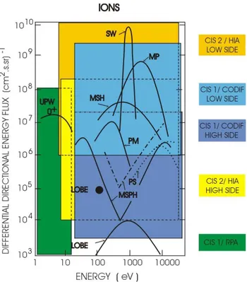
Fig. 1. Representative ion fluxes encountered along the Cluster orbit in the solar wind (SW), the magnetopause (MP), the magnetosheath (MSH), the plasma mantle (PM), the magnetosphere (MSPH), the plasma sheet (PS), the lobe and upwelling ions (UPW). The range of the different sensitivities of CIS1/CODIF (Low Side, High Side and RPA) and CIS2/HIA (Low g and High G) are shown with different colours.

– the upstream foreshock and solar wind dynamics; – the magnetic reconnection and the field-aligned current

phenomena;

– the study of low energy ionospheric population.

The four Cluster spacecraft encounter ionic plasma with vastly diverse characteristics over the course of one year (Fig. 1). In order to study all of the plasma regions with the fluxes shown in Fig. 1, the CIS experiment needs, therefore, to be a highly versatile and reliable ionic plasma experiment, with the following requirements:

– A very great dynamic range is necessary in order to

de-tect fluxes as low as those of the lobes, but also fluxes as high as solar wind fluxes, throughout the solar cycle.

– A broad energy range and a full 4 π angular coverage

are necessary to provide a satisfactory and uniform cov-erage of the phase space with sufficient resolution. The angular resolution must be sufficient to be able to sepa-rate multiple populations, such as gyrating or transmit-ted ions from the main population downstream of the bow shock, and be able to detect fine structures in the distributions.

(4)

H. R`eme et al.: First multispacecraft ion measurements in and near the Earth’s magnetosphere 1305

Table 1. CIS Flight Model (FM) Naming

CLUSTER - II Spacecraft Number Spacecraft Name Spacecraft Color and Line Style

Spacecraft FM CIS FM Number and Color

1 Rumba Black FM-5 (Phoenix) _FM-8_♦

2 Salsa Red First 2

spacecraft FM-6 FM-5 ♦

3 Samba Green launched FM-7 _FM-6_♦

4 Tango Magenta FM-8 _FM-7_♦

Spare: FM-4 (Phoenix)

– A high angular and energy resolution in a limited

en-ergy and angular range for the detection of cold beams, such as the solar wind, is required. Due to the limited energy range required, a beam tracking algorithm has been implemented in order to follow the beam in ve-locity space. Moreover, in the foreshock regions, for example, any study of backstreaming ions requires the simultaneous observation of the solar wind cold beam and of the backstreaming particles. Therefore, in con-junction with the solar wind coverage described above, a coverage of the entire phase space including the sun-ward sector with a broad energy range is also used.

– In the case of sharp boundaries, such as discontinuities,

it is necessary not to miss any information at the dis-continuity; thus, a very efficient means of mode change, which allows adaptation to the local plasma conditions, is provided.

– Moments of the three-dimensional (3D) distribution

(and of the sunward sector, in solar wind mode) are computed on board, with high time resolution to con-tinuously generate key parameters that are necessary for event identification.

– In order to study detailed phenomena of complex

mag-netospheric plasma physics, multiple particle popula-tions must be identified and characterized; therefore, a 3D distribution is needed. In order to transmit the full 3D distribution while overcoming the telemetry rate limitations, a compression algorithm has been intro-duced, which allows for an increased amount of infor-mation to be transmitted.

To achieve the scientific objectives, the CIS instrumenta-tion has been designed to simultaneously satisfy the follow-ing criteria on the four spacecraft:

– Provide uniform coverage of ions over the entire 4 π

steradian solid angle with good angular resolution.

– Separate the major mass ion species from the solar wind

and ionosphere, i.e. those which contribute significantly

Fig. 2. Cross sectional view of the HIA analyser.

to the total mass density of the plasma (generally, H+, He++, He+, and 0+).

– Have high sensitivity and large dynamic range (≥ 107) to support high time resolution measurements over the wide range of plasma conditions to be encountered in the Cluster mission (Fig. 1).

– Have high (5.6◦_×_5.6◦_{) and flexible angular sampling}

resolution to support measurements of ion beams and the solar wind.

– Have the ability to routinely generate on board the

fun-damental plasma parameters for major ion species, with one spacecraft spin time resolution (4 s). These param-eters include the density (n), velocity vector (V ), pres-sure tensor (P ), and heat flux vector (H ).

– Cover a wide range of energies, from spacecraft

poten-tial to about 40 keV/e.

– Have versatile and easily programmable operating

modes and data processing routines to optimize the data collection for specific scientific studies and widely vary-ing plasma regimes.

To satisfy all these criteria, the CIS package consists of two different instruments: a Hot Ion Analyser (HIA) sen-sor and a time-of-flight ion COmposition and DIstribution Function (CODIF) sensor. The CIS plasma package is ver-satile and is capable of measuring both the cold and hot ions of Maxwellian and non-Maxwellian populations (for exam-ple, beams) from the solar wind, the magnetosheath, and the magnetosphere (including the ionosphere) with sufficient an-gular, energy and mass resolutions to accomplish the scien-tific objectives. The time resolution of the instrument is suf-ficiently high to follow density or flux oscillations at the gy-rofrequency of H+ions in a magnetic field of 10 nT or less. Such field strengths can be frequently encountered by the Cluster mission. Oscillations of O+at the gyrofrequency can be resolved outside 6–7 RE. Hence, this instrument package

provides the ionic plasma data required to meet the Cluster science objectives (Escoubet and Schmidt, 1997).

(5)

1306 H. R`eme et al.: First multispacecraft ion measurements in and near the Earth’s magnetosphere

Fig. 3. Principle of the HIA anode sectoring.

3 The Hot Ion Analyser (HIA)

The Hot Ion Analyser (HIA) instrument combines the selec-tion of incoming ions according to the ion energy per charge by electrostatic deflection in a symmetrical, quadrispherical analyser which has a uniform angle-energy response with a fast imaging particle detection system. This particle imaging is based on microchannel plate (MCP) electron multipliers and position encoding discrete anodes.

3.1 Electrostatic analyser description

Basically, the analyser design is a symmetrical, quadrispher-ical electrostatic analyser which has a uniform 360◦

disc-shaped field of view (FOV) and an extremely narrow angular resolution capability. This symmetric quadrisphere or “top hat” geometry (Carlson et al., 1982) has been successfully used on numerous sounding rocket flights, as well as on the AMPTE/IRM, Giotto and WIND spacecraft (Paschmann et al., 1985; R`eme et al., 1987; Lin et al., 1995).

The symmetric quadrisphere consists of three concentric spherical elements. These three elements are an inner hemi-sphere, an outer hemisphere which contains a circular open-ing, and a small circular top cap which defines the entrance aperture. This analyser is classified as quadrispherical simply because the particles are deflected through 90◦. In the anal-yser, a potential is applied between the inner and outer plates and only charged particles with a limited range of energy and an initial azimuth angle are transmitted. The particle exit po-sition is a measure of the incident polar angle which can be resolved by a suitable position-sensitive detector system. The symmetric quadrisphere makes the entire analyser, including the entrance aperture, rotationally symmetric. The focusing characteristics are independent of the polar angle. We use the following convention: the angle about the spin axis is the az-imuth angle, whereas the angle out of the spin plane is called the polar angle.

The symmetrical quadrispherical analyser has good focus-ing properties, sufficient energy resolution, and the large

ge--5 0 5 0 1000 2000 3000 4000 5000

ALPHA ANGLE (DEG.)

COUNTS

CLU2-CIS2/FM5 FILE=5a800102 SECTOR=10 ENERGY=800 EV

0.8 0.9 1 1.1 0 0.2 0.4 0.6 0.8 1 HV ANALYZER (NORMALIZED) NORMALIZED RESPONSE -5 0 5 0 0.2 0.4 0.6 0.8 1

ALPHA ANGLE (DEG.)

NORMALIZED RESPONSE NORM= 1.006 FWHM(E)= 16.27 % D(E)= 19.55 % Emax= 1.008 HVmax= 103.8 Volts NORM= 1.018 FWHM(A)= 5.466 deg D(AL)= 6.565 deg ALmax= 0.6825 deg 19 May 98 \matlab\hia\matcis2.m

Fig. 4. Typical energy (top curves) and angular (bottom curve) res-olutions of the HIA analyser (flight model 5), for an energy beam of 800 eV; the energy resolution is about 19.6% and the intrinsic azimuthal resolution is about 6.6◦.

ometrical factor of a quadrisphere. Due to symmetry, it does not have the deficiencies of the conventional quadrisphere, namely the limited polar angle range and the severely dis-torted response characteristics at large polar angles, and it has an uniform polar response.

The HIA instrument has 2 × 180◦FOV sections parallel to the spin axis, with two different sensitivities and a ratio of about 25 (depending of the flight model and precisely known calibrations), corresponding, respectively, to the “high G” and “low g” sections. The “low g” section allows for the detection of the solar wind and the required high angular resolution is achieved through the use of 8 × 5.625◦central anodes, with the remaining 8 sectors having, in principle, a 11.25◦resolution; the 180◦“high G” section is divided into 16 anodes, 11.25◦each. In reality, sectoring angles are, re-spectively, ∼ 5.1◦ and ∼ 9.7◦, as demonstrated by calibra-tions (see Sect. 3.5). This configuration provides “instan-taneous”, 2D distributions sampled once per 62.5 ms (1/64 of one spin, i.e. 5.625◦ _{in azimuth), which is the nominal}

sweep rate of the high voltage applied to the inner plate of the electrostatic analyser to select the energy of the transmit-ted particles. For each sensitivity section, a full 4 π steradian scan is completed every spin of the spacecraft, i.e. 4 s, giv-ing a full, 3D distribution of the ions in the energy range of 5 eV e−1to 32 keV e−1(the analyser constant being ∼ 6.70). Figure 2 provides a cross sectional view of the HIA electro-static analyser. The inner and outer plate radii are 37.75 mm and 40.20 mm, respectively. The analyser has an entrance aperture which collimates the field of view, defines the two geometrical factors and blocks the solar UV radiation. 3.2 Detection system

A pair of half-ring microchannel plates (MCP) in a chevron pair configuration detects the particles at the exit of the

(6)

elec-H. R`eme et al.: First multispacecraft ion measurements in and near the Earth’s magnetosphere 1307

Table 2. Main features and measured parameters of the CIS experiment Full 3D ion distribution functions

Flux as a function of time, mass and pitch-angle

Moments of the distribution functions : density, bulk velocity, pressure tensor, heat flux vector Beams

Analysers Energy Range Energy Time Resolution Mass Resolution Angular Geometrical Factor Dynamics Distribution M/1M Resolution (Total) (cm2sec sr)−1

(FWHM) cm2.sr.keV/keV 2D 3D

ms s

Hot Ion Analyser ∼5 eV/e–32 keV/e 18% 62.5 4 – ∼5.6◦×5.6◦ 1.9 × 10−4for one half 104–2 × 1010 HIA 4.9.10−3for the other half

Ion Composition ∼0–38 keV/e 16% 125 4 ∼4–7 ∼11.2◦×22.5◦ 1.9× 10−2for one half 3.103–3.109 and Distribution 2.1×10−4for the other half

Function Analyser Mass range 3.0 × 10−2cm2sr for the

CODIF 1–32 amu RPA

Analysers Full Instantaneous Field of View Mass Power

(Nominal Operations) Hot Ion Analyser HIA 8◦×360◦ 2.45 kg 2.82 watts

Ion Composition 8◦×360◦ 8.39 kg 6.96 watts Function Analyser CODIF

CIS total raw CIS Total Weight: 10.84 kg without harness Average power: 9.78 watts

CIS Telemetry: ∼ 5.5 kbit/s

Expected total bit number (for the four spacecraft): 1012bits

trostatic analyser. The plates form a 2 × 180◦ ring shape, each 1 mm thick with an inter-gap of ∼ 0.02 mm, an inner diameter of 75 mm and an outer diameter of 85 mm. The MCPs have 12.5 µm straight microchannels, with a bias an-gle of 8◦ to reduce variations in MCP efficiency with az-imuthal direction. The chevron configuration, with double thickness plates, provides a saturated gain of 2 × 106, with a narrow pulse height distribution. The plates have a high strip current to provide a fast counting capability. For better detection, efficiency ions are post-accelerated by a ∼ 2300 V potential applied between the front of the first MCP and a high-transparency grid located ∼ 1 mm above. The anode collector behind the MCPs is divided into 32 sectors, each connected to its own pulse amplifier (Fig. 3). The main per-formances of the HIA sensor are summarised in Table 2. 3.3 Sensor electronics

Signals from each of the 32 MCP sectors are sent through 32 specially designed, very fast A121 charge-sensitive am-plifier/discriminators that are able to count at rates as high as

5 MHz. Output counts from the 32 sectors are accumulated in 48 counters (including 16 redundant counters for the so-lar wind), thus providing the basic anguso-lar resolution matrix according to the resolution of the anode sectoring.

According to the operational mode, several angular reso-lutions can be achieved:

– In the normal resolution mode, the full 3D distributions

are covered in ∼ 11.25◦angular bins (“high G” geomet-rical factor); this is the basic mode inside the magneto-sphere;

– In the high resolution mode the best angular resolution,

∼ 5.6◦×5.6◦, is achieved within a 45◦sector centred on the Sun direction, using the “low g” geometrical factor section; this mode is dedicated to the detection of the solar wind and near-ecliptic narrow beams.

3.3.1 High voltage power supplies

HIA needs a high-voltage power supply to polarise MCPs at

(7)

1308 H. R`eme et al.: First multispacecraft ion measurements in and near the Earth’s magnetosphere inner plate of the electrostatic analyser. The high voltages

to polarise the MCPs are adjustable under the control of the data processor system (DPS) microprocessor.

The energy/charge of the transmitted ions is selected by varying the deflection voltage applied to the inner plate of the electrostatic analyser, between 4800 and 0.7 V. The exponen-tial sweep variation of the deflection voltage is synchronised with the spacecraft spin period. The sweep should consist of many small steps that give effectively a continuous sweep. The counter accumulation time defines the number of energy steps, i.e. 31 or 62 count intervals per sweep. The covered energy range and the sweeping time are controlled by the onboard processor through a 12-bit DAC and a division in the two ranges for the sweeping high voltage. Therefore, the number of sweeps per spin, the amplitude of each sweep and the sweeping energy range can be adjusted according to the mode of operation (solar wind tracking, beam tracking, etc.). In the basic and nominal modes, the sweep of the total energy range is repeated 64 times per spin, i.e. once every 62.5 ms, giving a ∼ 5.6◦resolution in azimuth resolution. In the solar wind mode, HIA sweep is truncated when “high G” is facing the Sun in order to avoid the solar wind detection with “high

G” and to protect the MCP lifetime. 3.4 In-flight calibration test

A pulse generator can stimulate the 32 amplifiers that are un-der the processor control. In this way, important functions of the HIA instrument and of the associated on board process-ing can easily be tested. A special test mode is implemented for health checking of the microprocessor by making ROM check sums and RAM tests. The sweeping high voltage can be tested by measuring the voltage value of each individual step, and the MCP gain can be checked by occasionally step-ping MCP HV and by adjusting the discrimination level of the charge amplifiers. Performances of the HIA sensor are shown in Table 2 and in Fig. 1.

3.5 HIA performances

Pre-flight and extensive calibrations of all four HIA flight models and of the spare model were performed at the CESR vacuum test facilities in Toulouse, using large and stable ion beams of different ion species and variable energies, detailed studies of MCPs and gain level variations, MCP matching, and angular-energy resolution for each sector from a few tens of eV up to 30 keV. Typical performances of the HIA instru-ment are reproduced in Figs. 4, 5 and 6. Figure 4 shows an example of the typical energy and angular resolutions of the HIA analyser (flight model FM5/SC2) for an energy beam of 800 eV; in this case, the energy resolution is 16.3% and the intrinsic azimutal resolution ∼ 5.5◦. On average the analyser energy resolution 1E/E (FWHM) is ∼ 17%, almost inde-pendent of anode sectors and energy; thus the intrinsic HIA velocity resolution is ∼ 9%, only about half of the average solar wind spread value. This is equivalent to an angular resolution of ∼ 5◦and is thus, quite consistent with the

an-gular resolution capabilities of the instrument, i.e. ∼ 5.9◦

(FWHM) in the azimuthal angle, as indicated in Fig. 4, and

∼5.6◦_{in the polar angle. As seen in the example of Fig. 5 for}

the model FM6/SC3, the polar resolution stays, as expected, almost constant at ∼ 9.70◦over the 16 sectors (anodes 0 to 15) that constitute the “high G” section (Fig. 5). Anodes 16 to 31 correspond to the “low g” section and their response transmission is attenuated by a factor of about 25 (depend-ing on the flight model, see Table 3) due to the presence of a pin-hole grid placed in front of the 180◦collimator; the polar resolution of sectors 20 to 27 is ∼ 5.2◦. Figure 6 shows the excellent agreement for the transmission width for the four flight models and the spare model. Thus, when compared to the basic sectoring, ∼ 5.6◦and ∼ 11.2◦, all effective polar resolutions are reduced due to the existence of an insulation space between the discrete anodes, as well as by the presence of support posts within the field of view. Finally, experimen-tal energy, angle resolutions and transmission factors are in-troduced in the geometrical factor used to compute moments of the distribution function.

3.5.1 UV Rejection

A number of very interesting events are expected to occur when the HIA spectrometers face the Sun (2 times/spin): of course, the intense solar wind, but also, for example, tailward ion beams flowing along the Plasma Sheet Boundary Layer (PSBL). A number of measures were applied in order to sup-press or limit the solar UV contamination. Part of the UV is rejected by the entrance collimator; moreover, the inner sur-face of the outer sphere is scalloped and both spheres (and all internal parts) are treated and coated with a special black cupric sulfide. Extensive vacuum chamber tests of the HIA analysers were performed, using a calibrated continuous dis-charge source for extreme UV at He-584 ˚A and Lα 1215 ˚A lines. Reduction of the solar UV light reflectance at the Lα line was demonstrated in R`eme et al. (1997) for Cluster-1 flight models. The resulting maximum count rate recorded by the sunward looking sector (11.2◦wide) for these models was about 80 counts s−1(for an intensity equivalent to 3 Sun intensity units), and the UV contamination was distributed over about ∼ 100◦ in the polar angle; this UV contamina-tion was judged acceptable. Figure 7a shows this UV con-tamination for a Cluster-1 HIA flight model. However, for Cluster-2 flight models, it was decided to improve the UV rejection by changing the scalloping of the outer sphere. The result was excellent. Figure 7b shows the UV test result for the FM4 spare model under the same conditions as that of Fig. 7a for Cluster-1. The contamination is divided by a fac-tor of about 700. In Fig. 8, an example of measurements by the HIA FM6/SC3 instrument in the central plasma sheet on 11 September 2000 is shown. “Natural counts” are detected between about 150 eV and 14 keV. The UV rejection is ex-cellent since there are no counts in the Sun direction (+ and

−180◦) for the highest energy ion measurements where no natural particles are present in this region. In the same fig-ure, the absence of counts at the lowest and highest energies,

(8)

H. R`eme et al.: First multispacecraft ion measurements in and near the Earth’s magnetosphere 1309 100 1000 10000 100000 -90 -75 -60 -45 -30 -15 0 15 30 45 60 75 90 105 120 135 150 165 180 195 210 225 240 255 270

beta angle (deg)

counts/sec

0 15

16 20 27 31

5 10

Fig. 5. Relative transmission of the 16 HIA High G (from 270◦to 90◦) and 16 HIA Low g (from 90◦to −90◦) polar sectors (see Fig. 3) for FM6 at 5 keV. 0.000 2.000 4.000 6.000 8.000 10.000 12.000 0 1 2 3 4 5 6 7 8 9 10 11 12 13 14 15 16 17 18 19 20 21 22 23 24 25 26 27 28 29 30 31 sector

transmission width (deg)

FM4 FM5 FM6 FM7 FM8

Fig. 6. Beta sector transmission of HIA for the four flight models and the spare model. Results are very similar for the five models. Sectors 0–15 correspond to the High G and 16–31 correspond to the low g. Transmission in sectors 20–27 is divided by two, as expected from the geometry.

i.e. below and above the central plasma sheet, particle en-ergies show that the HIA sensors have a very low MCP and amplifier noise.

4 The ion composition and distribution function anal-yser (CODIF)

The CODIF instrument is a high-sensitivity, mass-resolving spectrometer with an instantaneous 360◦×8◦field of view to measure complete 3D distribution functions of the major ion species within one spin period of the spacecraft. Typ-ically, these include H+, He++, He+ and O+. The sen-sor primarily covers the energy range between 0.02 and 38 keV/charge. With an additional Retarding Potential Anal-yser (RPA) device in the aperture system of the sensor with

pre-acceleration for energies below 25 eV/e, the range is ex-tended to energies as low as the spacecraft potential. Hence, CODIF covers the core of all plasma distributions of impor-tance to the Cluster mission.

To cover the large dynamic range required for accurate measurements in the low-density plasma of the magneto-tail and the dense plasma in the magnetosheath/cusp/ bound-ary layer, it is mandatory that CODIF employ two different sensitivities. The minimum number of counts in a distribu-tion needed for computing the basic plasma parameters, such as the density, is about 100. These must be accumulated in 1 spin in order to provide the necessary time resolution. However, the maximum count rate which the time-of-flight system can handle is ∼ 105 counts s−1 or 4 × 105 counts spin−1. This means that the dynamic range achievable with

(9)

Table 3. Energy resolution, analyser constant and geometrical factor per anode for the four HIA flight models and for the spare model. The high geometrical factor corresponds to sectors 0–15 and the low geometrical factor corresponds to sectors 20–27 (see Fig. 3). These parameters are slightly different from the parameters of the Cluster-1 models due to the modification of the sphere scalloping design used to obtain a better UV rejection (see below)

Parameter FM5/SC2 FM6/SC3 FM7/SC4 FM8/SC1 FM4/SPARE Geometrical G g G g G g G g G g Factor Attenuation 1 1/24 1 1/22 1 1/25 1 1/25 1 grid 1E/E,% 16.44 15.94 16.66 15.96 17.61 17.23 16.59 16.07 17.19 17.32 Kanalyser 7.629 7.341 7.042 7.685 7.454 (all sectors) Geometrical Factor per 3.00 5.769 3.805 1.084 3.403 6.368 4.966 1.226 anode ×10−4 ×10−6 ×10−4 ×10−5 ×10−4 ×10−6 ×10−4 ×10−5 (cm2.sr.keV/ keV) 0 200 400 600 800 1000 1200 1400 -15 -10 -5 0 5 10 15 α angle (deg.) COUNTS (/5sec) Sector 6 Sector 7 Sector 8 0 5 10 15 20 25 -15 -10 -5 0 5 10 15

alpha angle (deg)

COUNTS (/min)

sector 6 sector 7 sector 8

Fig. 7. UV effects on a Cluster-1 HIA model (counts/5 s) in Fig. 7(a) and on a Cluster-2 HIA model (counts/min) in Fig. 7( b) in the function of the polar angle. The background for Cluster-2 has been divided by two orders of magnitude by improving the analyser scalloping.

(10)

Spacecraft n°3

Perfect UV

Rejection

CPS:Isotropic

Distributions

Low MCP+Amp

Noise

Fig. 8. Example of in-flight measurements of HIA on spacecraft 3 in the central plasma sheet on 11 September 2000. Each rectangle is a

2–8 plot, 2, in ordinate, ranging from −90◦to +90, 8, in abscissa, ranging from 180◦to +180◦, with the sunward direction at (2, 8) = (0◦, ±180◦). Each line corresponds to 1 of the 16 logarithmically spaced energies between 24.3 eV (bottom line) to 34 117.3 eV. Ten successive measurements are shown (one by column). There is no Sun effect in the detector.

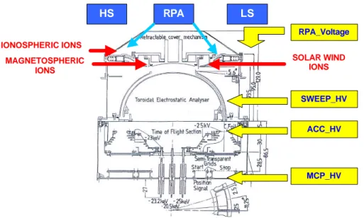
LS RPA MAGNETOSPHERIC IONS SOLAR WIND IONS SWEEP_HV MCP_HV ACC_HV HS IONOSPHERIC IONS RPA_Voltage

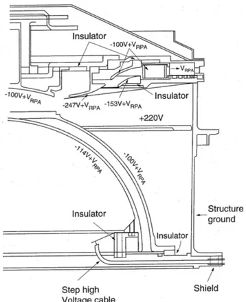
Fig. 9. Cross sectional view of the CODIF sensor. The voltages in the TOF section are shown for a 25 kV post-acceleration.

a single sensitivity is only 4 × 103.

Figure 1 shows the fluxes covered by CODIF, ranging from magnetosheath/magnetopause protons to tail lobe ions (which consists of protons and heavier ions); fluxes from

∼103 to over 108 must be covered, requiring a dynamic range of larger than 105. This can only be achieved if CODIF incorporates two sensitivities, differing by a factor of about 100. Therefore, CODIF consists of two sections, each with

a 180◦field of view, with different (by a factor of 100) ge-ometrical factors. In this way, one section always has count rates which are statistically meaningful and at the same time, the section can be handled by the time-of-flight electronics. The exception is solar wind H+which often saturates the in-strument, but is measured with the small g of HIA.

The CODIF instrument combines the ion energy per charge selection by deflection in a rotationally symmetric

(11)

Fig. 10. Geometry of the CODIF RPA.

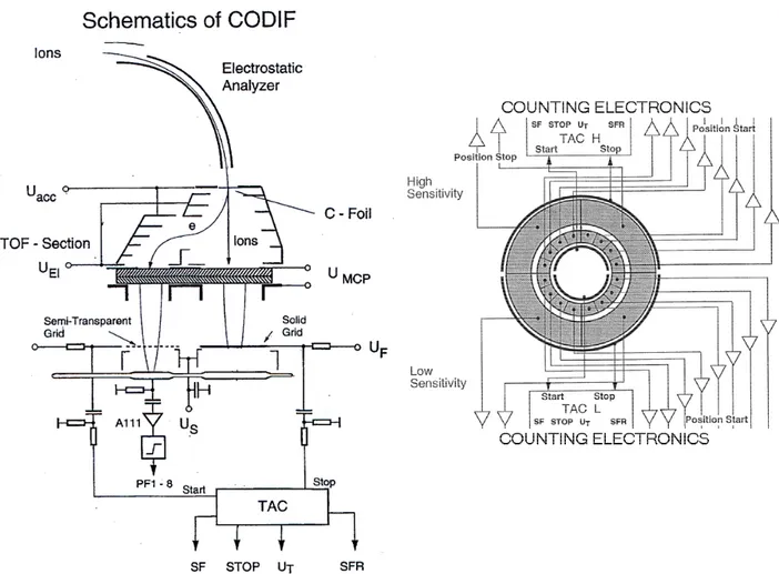
toroidal electrostatic analyser with a subsequent time-of-flight analysis after post-acceleration to ≥ 15 keV/e. A cross section of the sensor showing the basic principles of opera-tion is presented in Fig. 9. The energy-per-charge analyser is of a rotationally symmetric toroidal type, which is basi-cally similar to the quadrispheric top-hat analyser used for HIA. It has a uniform response over 360◦of the polar angle. The energy per charge selected by the electrostatic analyser

E/Q, combined with the energy gained by post-acceleration

e.UACC, and the measured time-of-flight through the length

d of the time-of-flight (TOF) unit, τ , yield the mass per charge of the ion M/Q according to:

M/Q =2(E/Q + e · UACC)/(d/τ )2·α.

The quantity α represents the effect of energy loss in the thin carbon foil (∼ 3 µg cm−2_{) at the entry of the TOF section}

and this depends on the particle species and incident energy. 4.1 Electrostatic analyser description

The electrostatic analyser (ESA) has a toroidal geometry which provides optimal imaging just past the ESA exit. This property was first demonstrated by Young et al. (1988). The ESA consists of inner and outer analyser deflectors, a top-hat cover and a collimator. The inner deflector consists of toroidal and spherical sections which join at the outer deflec-tor entrance opening (angle of 17.9◦). The spherical section has a radius of 100 mm and extends from 0 to 17.9◦ about

the Z-axis. The toroidal section has a radius of 61 mm in the poloidal plane and extends from 17.9◦_{to 90}◦_{. The outer}

de-flector covers the toroidal section and has a radius of 65 mm. The top-hat cover consists of a spherical section with a ra-dius of 113.2 mm, which extends from 0 to 16.2◦. Therefore, fits inside the entrance aperture of the outer deflector. The outer deflector and the top-hat cover are at signal ground un-der normal operation, but are biased at about −100 V during RPA operation. The inner deflector is biased with voltages varying from −1.9 to −4950 V in order to cover the energy range in a normal ESA operation. These are set to about

−113 V for the RPA.

The fact that the analyser has a complete cylindrical sym-metry provides the uniform response in the polar angle. A beam of parallel ion trajectories is focused to a certain loca-tion at the exit plane of the analyser. The exit posiloca-tion, and thus the incident polar angle of the ions, is identified by using the information from the start detector (see Sect. 3.2). The full angular range of the analyser is divided into 16 channels of 22.5◦each. The broadening of the focus at the entrance of the TOF section is small compared to the width of the angular channels.

As illustrated in Fig. 9, the analyser is surrounded by a cylindrical collimator which serves to define the acceptance angles and restricts UV light. The collimator consists of a cylindrical can with an inner radius of 96 mm. The entrance is covered by an attenuation grid with a radius of 98 mm which is kept at spacecraft ground. The grid has a 1% trans-mission factor over 50% of the analyser entrance and > 95% transmission over the remaining 50%. The high transmis-sion portion extends over the azimuthal angle range of 0◦_to

180◦_{where 0}◦_{is defined along the spacecraft spin axis. The}

low transmission portion, whose active entrance only extends from 22.5◦ to 157.5◦ in order to avoid the counting of any crossover from the other half, has a geometric factor that is reduced by a factor of ≈ 100 in order to extend the dynamic range to higher flux levels. On the low-sensitivity half, the collimator consists of a series of 12 small holes, vertically spaced by approximately 1.9◦ around the cylinder. These apertures have acceptance angles of 5◦FWHM, so there are no gaps in the polar angle coverage. The ion distributions near the polar axis are highly over-sampled during one spin relative to the equatorial portion of the aperture. Therefore, count rates must be weighted by the sine of the polar angle to normalise the solid-angle sampling for the moment calcu-lations and 3D distributions.

The analyser has a characteristic energy response of about 7.6, and an intrinsic energy resolution of 1E/E ∼= 0.16. The entrance fan covers a viewing angle of 360◦in the po-lar angle and 8◦in the azimuth. With an analyser voltage of 1.9–4950 V, the energy range for ions is 15–38 000 eV/e. The deflection voltage is varied in an exponential sweep. The full energy sweep with 30 contiguous energy channels is per-formed 32 times per spin. Thus, a partial two-dimensional cut through the distribution function in the polar angle is ob-tained every 1/32 of the spacecraft spin. The full 4π ion distributions are obtained in a spacecraft spin period.

(12)

Fig. 11. The CODIF sensor: schematics (left) and MCP sectoring (right).

The outer plate of the analyser is serrated in order to mini-mize the transmission of scattered ions and UV, for the same reason the analyser plates are covered with a copper black coating. Behind the analyser, the ions are accelerated by a post-acceleration voltage of −14 to −25 kV, such that ther-mal ions also have sufficient energy before entering the TOF section. After the first in-flight tests, this high voltage has been set at −15 kV in all of the spacecraft, giving good re-sults and safe use of CODIF.

4.2 Retarding Potential Analyser

In order to extend the energy range of the CODIF sensor to energies below 15 eV/e, an RPA assembly is incorporated in the two CODIF apertures (see Fig. 10). The RPA provides a way of selecting low-energy ions as input to the CODIF anal-yser without requiring the ESA inner deflector to be set accu-rately near 0 V. The RPA collimates the ions, provides a sharp low-energy cutoff at a normal incident grid, pre-accelerates the ions to 100 eV after the grid, and deflects the ions into the ESA entrance aperture. The energy pass of the ESA is about 5–6 eV at 100 eV of pre-acceleration, assuming all deflection voltages are optimised. This energy pass is very sensitive to the actual RPA deflection optics, so that deflection voltages have to be determined at about the 1% level.

The RPA assembly consists of a collimator, an RPA grid and pre-acceleration region, and deflection plates. The col-limator section is kept at spacecraft ground. When the RPA is active, only RPA measurements are produced by CODIF. The RPA can be thought of as a separate ion optics front end for CODIF, which can be used in on command, thereby re-placing the normal ion optics. A separate RPA aperture ring defines a field of view parallel to the normal CODIF field of view, but displaced towards the analyser top by about 15 mm. As with normal CODIF operations, the field of view extends 180◦in azimuth on one side of the analyser and 135◦on the other side. Only one side can be active at a time. Unlike the normal CODIF entrance aperture, both sides of the RPA have the same sensitivity; there is no attenuation grid on one half to reduce the effective geometric factor for the RPA.

When the RPA is enabled, the normal entrance aperture is closed off by a positively biased grid, which pushes ions near 100 eV/e away from the entrance slot below the top cap. Although higher energy ions could still enter this slot, the bias between hemispheres is set to pass energies only near 100 eV/e, so that higher energy ions strike the inner hemisphere, and fail to traverse the analyser gap to exit the ring. A retarding grid at the RPA entrance rejects ions with energy/charge below the set threshold voltage and allows

(13)

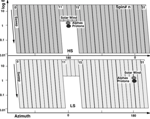
Fig. 12. Energy sweeping scheme of CODIF in the solar wind. The sweep is shown in the log E versus the azimuthal angle for the high-sensitivity section (upper panel) and low-high-sensitivity section (lower panel), starting at the high energy end. When looking into the solar wind, the sweep stops above the alpha particles for the high-sensitivity section but the sweep does not stop for the alpha particles and the protons for the low-sensitivity section.

higher energy/charge ions to pass. The accepted ions are first collimated and accelerated by 100 volts, and then routed by three deflector surfaces into the main entrance slot. The hemispherical analyser filters out the higher energies from the incoming beam and the remainder enter the TOF section for a velocity measurement. The deflection system provides a method of steering the RPA low-energy ions into the CODIF ESA.

The RPA grid and pre-acceleration region consist of a pair of cylindrical rings, sandwiched between resistive ceramic material. Both inner and outer cylindrical rings contain aper-tures separated by posts every 22.5◦, similar to the ESA colli-mator entrance, in order to allow the ions to pass through the assembly. The RPA grid is attached to the inner surface of the outer cylindrical ring. This outer ring has a small ledge which captures the RPA grid and which also provides the initial op-tical lens that is crucial to the RPA operation. Both inner and outer cylindrical rings are in good electrical contact with the resistive kapton (silver epoxy). During RPA operation, the outer cylindrical ring is biased from spacecraft ground to about +25 V, and provides the sharp, low-energy RPA cut-off. This voltage is designated Vrpa in Fig. 10. The inner

cylindrical ring tracks the outer ring voltage and is biased at

−100 V + Vrpa. The inner cylindrical ring, the ESA outer

deflector, and the ESA top-hat cover are electrically tied to the RPA deflector.

The RPA deflection plates consist of three toroidal

deflec-tors located above the ESA collimator entrance and one de-flector disk located below the collimator entrance. The three toroidal deflectors are used to deflect the ions into the ESA. The deflector disk is used to prevent low-energy ions from entering the main aperture and to collect any photoelectrons produced inside the analyser, while in RPA mode.

4.3 Time-of-flight and detection system

The CODIF sensor uses a time-of-flight technology (M¨obius et al., 1985). The specific parameters of the time-of-flight spectrometer have been chosen such that a high detection ef-ficiency of the ions is guaranteed. High efef-ficiency is not only important for maximizing the overall sensor sensitivity, but it is especially important for minimising false mass identifica-tion resulting from false coincidence at a high counting rate. A carbon foil, that is too thin, would result in a significant reduction in the efficiency of secondary electron production for the “start” signal, while an increase in thickness does not change the secondary electron emission significantly (Rit-ter, 1985). Under these conditions, a post-acceleration of

≥14 kV is necessary for the mass resolution of the sensor. After passing the ESA, the ions are focused onto a plane close to the entrance foil of the time-of-flight section (Fig. 11). The TOF section is held at the post-acceleration potential in order to accelerate the ions into the TOF section, where the velocity of the incoming ions is measured. The flight path of the ions is defined by the 3 cm distance between

(14)

Total Effic (Adjusted) vs. Total Energy

0 0.1 0.2 0.3 0.4 0.5 0.6 0.7 0.8 0.9 1 0 5 10 15 20 25 30 35 40 45 50 55 60

Total Energy (keV)

1 2 3 4 5 6 7 8 Fit FM7 (Bern 03 04 1999) Ion: H+ MCP: 8C

0 0.1 0.2 0.3 0.4 0.5 0.6 0.7 0.8 0.9 1 0 5 10 15 20 25 30 35 40 45 50 55 60

10 11 12 13 14 15 LS_Fit HS_Fit

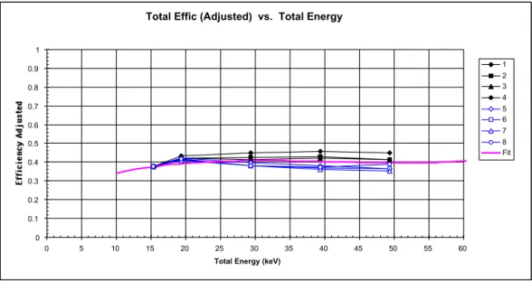
Fig. 13. CODIF FM7 High Side normalised total efficiency verses total energy for H+for the different anodes and with a general fit (upper curve) and CODIF FM7 Low Side normalised total efficiency verses total energy for H+for the different anodes and with a general fit; High Side fit of the upper curve is added (lower curve).

the carbon foil at the entrance and the surface of the “stop” microchannel plate (MCP). The start signal is provided by secondary electrons, which are emitted from the carbon foil during the passage of the ions. The entrance window of the TOF section is a 3 µg cm−2 carbon foil, which has an op-timum thickness between the needs of low-energy loss and straggling in the foil, and high efficiency for secondary elec-tron production. The elecelec-trons are accelerated to 2 keV and deflected onto the start MCP assembly by a suitable potential configuration.

The secondary electrons also provide the position infor-mation for the angular sectoring. The carbon foil is made up

of separate 22.5◦ _{sectors, separated by narrow metal strips.}

The electron optics are designed to strongly focus secondary electrons, originating at a foil, onto the corresponding MCP start sector.

The MCP assemblies (Fig. 11) are ring-shaped with inner and outer radii of 6 × 9 cm and 3 × 5 cm for the stop and start detectors, respectively. For the start signals, the out-put of the MCPs is collected on a set of segmented plates behind the MCPs (22.5◦each), and on thin wire grids with

≈50% transmission at a distance of 10 mm in front of the signal plates. The stop signals are collected through a solid, non-transparent grid (and not through a semitransparent grid,

(15)

0 0.1 0.2 0.3 0.4 0.5 0.6 0.7 0.8 0.9 1 0 5 10 15 20 25 30 35 40 45 50 55 60

1 2 3 4 5 6 7 8 Fit

0 0.1 0.2 0.3 0.4 0.5 0.6 0.7 0.8 0.9 1 0 5 10 15 20 25 30 35 40 45 50 55 60

10 11 12 13 14 15 LS Fit HS fit

Fig. 14. CODIF FM7 High Side normalised total efficiency verses total energy for He+for the different anodes and with a general fit (upper curve) and CODIF FM7 Low Side normalised total efficiency verses total energy for He+for the different anodes and with a general fit; High Side fit of the upper curve is added (lower curve).

such as for Cluster-1), improving significantly the H+ detec-tion efficiency. All are at ground potential (see Fig. 9). Thus, almost all of the post-acceleration voltage is applied between the rear side of the MCPs and the signal anodes. The tim-ing signals are derived from the 50% transmission grids, and separately derived for the high- and the low-sensitivity TOF section. The position signals, providing the angular infor-mation in terms of 22.5◦sectors, are derived from the signal plates behind the start MCP. The main performances of the CODIF sensor are summarised in Table 2.

4.4 Sensor electronics

The sensor electronics of the instrument consist of two time-to-amplitude converters (TACs) to measure the time-of-flight of the ions between the start carbon foil and the stop MCPs, two sets of eight position discriminators at the start MCPs, two sets of two position discriminators at the stop MCPs, and the event selection logic. Each individual ion is pulse-height-analysed according to its time-of-flight incidence in azimuthal (given by the spacecraft spin) and the polar angle (given by the start position), and the actual deflection voltage.

(16)

0 0.1 0.2 0.3 0.4 0.5 0.6 0.7 0.8 0.9 1 0 5 10 15 20 25 30 35 40 45 50 55 60

1 2 3 4 5 6 7 8 Fit FM7 (Bern 03 06 1999) Ion: 0+ MCP: 8C with 92

0 0.1 0.2 0.3 0.4 0.5 0.6 0.7 0.8 0.9 1 0 5 10 15 20 25 30 35 40 45 50 55 60

10 11 12 13 14 15 Fit HS_Fit

Fig. 15. CODIF FM7 High Side normalized total efficiency verses total energy for O+for the different anodes and with a general fit (upper curve) and CODIF FM7 Low Side normalised total efficiency verses total energy for O+for the different anodes and with a general fit; High Side fit of the upper curve is added (lower curve).

The eight position signals for each TOF section (one TOF section for the Low Side, one TOF for the High Side, see Fig. 11), in order to achieve the 22.5◦resolution in the po-lar angle, are independently derived from the signal anodes, while the timing signals are taken from the grids in front of the anodes. Likewise, the stop MCPs, consisting of four in-dividual MCPs, are treated separately to carry along partial redundancy. By this technique, the TOF and the position signals are electrically separate in the sensor. The position pulses are fed into charge-sensitive amplifiers and identified by pulse discriminators, the signal of which is directly fed into the event selection logic. The TOF unit is divided into two TOF channels.

The conditions for valid events are established in the event-selection logic. The respective coincidence conditions can be changed via ground command. Several count rates are accumulated in the sensor electronics. There are monitor rates of the individual start and stop detectors to allow for the continuous monitoring of the carbon foil and MCP per-formance. The total count rates of TOF coincidence show the valid events accumulated for each TOF section. These rates can be compared with the total stop count rates in or-der to monitor in-flight the efficiency of the start and stop assemblies.

In order to protect the MCPs, the solar wind protons and the solar wind alpha particles are blocked from detection by

(17)

1318 H. R`eme et al.: First multispacecraft ion measurements in and near the Earth’s magnetosphere FM7 15 keV 0 50 100 150 200 tof channel 0.0 0.2 0.4 0.6 0.8 1.0 counts 20 keV 0 50 100 150 200 tof channel 0.0 0.2 0.4 0.6 0.8 1.0 counts 30 keV 0 50 100 150 tof channel 0.0 0.2 0.4 0.6 0.8 1.0 counts 40 keV 0 20 40 60 80 100 tof channel 0.0 0.2 0.4 0.6 0.8 1.0 counts 50 keV 0 20 40 60 80 100 tof channel 0.0 0.2 0.4 0.6 0.8 1.0 counts

Fig. 16. CODIF FM7 time-of flight spectra for the four major species at 5 energies. The spectra are averaged over all positions. The vertical lines show the thresholds used to distinguish species.

a simple scheme during the sweeping cycle, as shown in Fig. 12 (actually there are four consecutive sweeps that are modified when G is facing the solar wind, whereas they are not modified when g is facing the solar wind). The sweep, starting at high energies, is shown for the high-sensitivity section in the upper panel and for the low-sensitivity sec-tion in the lower panel in log E and the azimuthal angle. The voltage sweep, which starts at high energies, is stopped above the alphas when the high-sensitivity section is facing the solar wind. The result is a small data gap for both sec-tions of the sensor simultaneously. The primary purpose for introducing this scheme is to avoid a short-time gain depres-sion of the MCP area, which would otherwise persist on the order of 1 s after the impulsive high count rate that would result from the solar wind.

4.4.1 High voltage system

A sweep-voltage, high-voltage power supply generates an exponential voltage waveform from 1.9 to 4950 V for the electrostatic analyser. A ≥ 14 kV static supply feeds the post-acceleration voltage, which can be adjusted via ground com-mand. Another adjustable supply is used for the MCPs and

FM7 Ion Spillover 10 20 30 40 50 60 Total Energy 0.001 0.010 0.100 1.000 Fraction H+ < H+ H+ He++ He+ mid O+ >O+ 10 20 30 40 50 60 Total Energy 0.001 0.010 0.100 1.000 Fraction He++ 10 20 30 40 50 60 Total Energy 0.001 0.010 0.100 1.000 Fraction He+ 10 20 30 40 50 60 Total Energy 0.001 0.010 0.100 1.000 Fraction O+

Fig. 17. Example of ion spillover effect in CODIF FM7: fraction of each 4 major ion species detected in the H+, He++, He+, and O+ bins.

the collection of secondary electrons. It supplies up to 5 kV and is floated on top of the post-acceleration voltage. 4.5 In-flight calibration

Upon command, an in-flight-calibration (IFC) pulse genera-tor can stimulate the two independent TOF branches of the electronics according to a predefined program. Within this program, all important functions of the sensor electronics and the subsequent on board processing of the data can be automatically tested. Temporal variations of calibration pa-rameters can be measured. The in-flight calibration can also be triggered by ground command in a very flexible way, e.g. for trouble shooting purposes. In addition, the known promi-nent location of the proton signal can, if necessary, serve as a tracer of changes in the sensor itself.

4.6 CODIF performances

4.6.1 Resolution in mass per charge

The instrumental resolution in mass per charge is determined by a combination of the following effects:

(18)

Magnetopause

Fig. 18. Comparison of the electron density measured by the Whisper instrument and the ion density measured by HIA, on 19 December 2000 when the spacecraft 3 leaves the magnetosphere and moves into the magnetosheath. At the top are the ion fluxes, at the bottom are the wave measurements of Whisper and in the middle is the density measured by HIA and three-points deduced from the Whisper measurements. The agreement is excellent. Before the magnetopause traversal, the density is too small to be evaluated by Whisper.

– Energy resolution of the electrostatic deflection analyser

(1E/E = 0.16);

– TOF dispersion caused by the angular spread of the ion

trajectories due to the characteristics of the analyser and the straggling in the carbon foil (the angular spread of = 13◦leads to 1τ/τ = 0.03);

– TOF dispersion caused by energy straggling in the

car-bon foil (1τ/τ ) up to 0.08 for 25 keV O+);

– Electronic noise in the TOF electronics and

secondary-electron flight time dispersion (typically 0.3 ns). The resulting TOF dispersion amount,(1τ/τ ) ≤ 0.1, fi-nally leads to a M/Q resolution between 0.15 for H+_{, and}

0.25 for low energy O+_.

4.6.2 CODIF calibrations

The TOF efficiency is a function of the ion species and the total energy, which is the sum of the original ion energy plus the energy gained in the post-acceleration potential. The to-tal efficiency for measuring an ion in CODIF is determined by the efficiency of the “Start” signal, the efficiency of the “Stop” signal, and the efficiency of “Valid Single Events”. The “Start” efficiency is a function of the number of sec-ondary electrons emitted from the carbon foil, the focusing

of the electrons onto the MCP, the MCP active area, and the MCP gain and MCP signal threshold. It is measured using the ratio of the Start-Stop Coincidence rate (SFR) to the “Stop” rate (SR). The “Stop” efficiency is a function of the scattering of the ion in the foil (which can scatter it away from the active area), the MCP active area, and the MCP gain and signal threshold. It is given by the ratio of the SFR rate to the “Start” rate, SF. In order for an ion to be counted as a valid event, it must generate not only a start and stop signal, but also a single “Start Position” (PF) signal. The “Valid Event Efficiency” is given by the ratio of the Valid Single Event rate, SEV, to the SFR. These efficiencies are all a function of energy and species, as well as MCP voltage. Determining the final efficiencies is done in two steps. First, the optimum voltage at which to run the MCPs is determined. Then, using the optimum MCP voltage, the efficiencies for each species as a function of energy and position are determined.

Each CODIF model, including the spare model, has been very well calibrated (see Table 4). The results for CODIF CIS model FM7, on spacecraft 4, are presented here as an example. For the other models, see the full report of Kistler (2000).

To determine ion efficiencies verses energy, once the opti-mum MCP voltage is set, data are collected over a range of beam energies. The total ion efficiency is a function of to-tal ion energy (original beam energy plus post-acceleration).

(19)

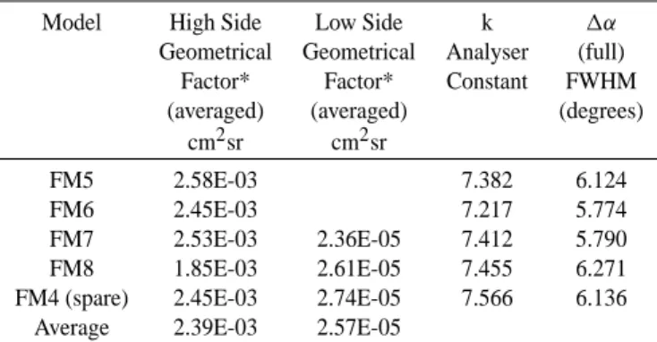
Table 4. Summary of the geometric factors for one instrument po-sition (out of 8 for High Side and 6 for Low Side), and energy and angle response for the CODIF instruments deduced from all cali-bration data

Model High Side Low Side k 1α

Geometrical Geometrical Analyser (full) Factor* Factor* Constant FWHM (averaged) (averaged) (degrees)

cm2sr cm2sr

FM5 2.58E-03 7.382 6.124 FM6 2.45E-03 7.217 5.774 FM7 2.53E-03 2.36E-05 7.412 5.790 FM8 1.85E-03 2.61E-05 7.455 6.271 FM4 (spare) 2.45E-03 2.74E-05 7.566 6.136

Average 2.39E-03 2.57E-05

Even when the instrument is operating at the optimum MCP voltage, there is a significant difference between the final effi-ciencies measured at different positions (pixels). Thus, it was necessary to determine the final ion efficiencies as a function not only of energies and species, but also of position.

Figures 13, 14 and 15 are plots of the total adjusted ion efficiencies verses total beam energy on both the High Side (HS) and Low Side (LS) for H+, He+, and O+ ions. The efficiency for He++is the same as for He+at the same total energy (not energy per charge). Since He++ goes to twice the energy, we did separate curve fits for He++(not shown) to assure that the curves were stable at higher energies.

Figure 16 shows the time-of-flight spectra over a range of energies for FM7. This figure is assembled from many data sets using individual species. The relative heights of the peaks depend on the beam intensity and length of the run, and, therefore, have no significance for this analysis. The vertical lines show the thresholds used to distinguish the species. During commissioning, it was found that a large peak can be observed in the lowest channel, and during time periods with a high oxygen flux, there is a second peak be-low the proton peak which seems to be correlated with the O+ flux. It is probably due to ions with a time-of-flight greater than the allowed 200 ns from the long O+ tail. To keep these spurious peaks from being counted with the pro-tons, a threshold below the H+peak was introduced.

The mass resolution of the CODIF instrument is defined by the resolution in time-of-flight. The width of the peaks in time-of-flight is determined by the spread in energy that re-sults from the energy loss in the carbon foil and any noise in the time-of-flight electronics. Since the energy loss is a sta-tistical process, ions that enter the foil with one energy come out with a range of energies. The percentage of energy that is lost is the worst for low-energy ions and heavy ions. The electronic noise in the time-of-flight circuit is independent of ion energy. Since the loss in the carbon foil is a smaller frac-tion of the total energy, the peaks should become narrower with increasing energy. This is evident in the O+peaks, but not so clear for the lower mass peaks. One reason for this is

that there is a significant difference between the locations of the peaks for different positions. Since the peaks move closer together with energy, but the width of the low mass ions does not significantly improve, there are more problems with over-lapping peaks, and, therefore, worse mass resolution at high energies. The bin with the most overlap with other species is the He++bin. A quantitative analysis of the spill-over be-tween bins is shown in Fig. 17. Each panel shows the fraction of a particular species that is classified in a particular mass bin. The thresholds were chosen to maximize the percentage of an ion that falls into the correct bin, but also to minimize the percentage of H+ions that fall into the wrong bin. This is particularly important at the H+/He++ boundary. Since there is usually much more H+than He++in space plasmas, a small percentage of H+spilling into the He++bin can sig-nificantly effect the He++_{measurement. In this case, about}

3.5% of the H+_{ions fall into the He}++_{bin, and 70% of the}

He++ _{ions are in the He}++ _{bin. For O}+_{, the fraction that}

falls into the O+ bin was kept low at low-energies in order to reduce the background in the bin. At 15 keV, the O+has a long tail extending to high TOF channels. The background from accidental coincidences in a bin is proportional to the number of TOF channels in the bin, so there is an advantage to keeping a narrow bin, even if some of the real signal is lost.

The RPA geometric factor and energy response has also been calibrated (McCarthy, 2000). For the group of 8 anodes when the high sensitivity side is enabled, the total RPA ge-ometric factor is 3.0 × 10−2cm2.sr. It is 2.2 × 10−2cm2.sr for the group of 6 anodes when the low sensitivity side is enabled.

4.6.3 Dynamic range

The design of the electrostatic analyser guarantees a large geometrical factor in the high-sensitivity section

A.1E/E.1τ.π = 0.025 cm2.sr. The energy bandwidth

is 1E/E = 0.16. The efficiency of the TOF unit is about 0.5. Differential energy fluxes as low as ∼ 3 × 103ions s−1cm−2sr−1 can be detected by the instrument with the full time resolution of 1 spin period and about 5 counts of the energy−1channel. The sensitivity is increased accordingly for longer integration time . Therefore, the dy-namic range reaches seven decades. The upper flux limit of the instrument amounts to 3 × 109ions s−1cm−2sr−1, which leads to a count rate of 105counts s−1in one TOF unit (near the saturation of the analysing electronics) and still guaran-tees a mass density determination with better than a 10% ac-curacy for the reduced aperture geometry.

5 Data processing system

CIS data can be collected in a variety of modes with different bit-rates: 5527 bit/s in mode NM1 (normal mode), 6521 bit/s in mode NM2 (ion mode), 4503 bit/s in mode NM3 (elec-tron mode, with the PEACE instruments having more bits

(20)

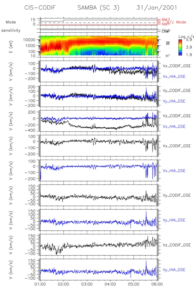
Fig. 19. Example showing the importance of the calibrations, from top to bottom: instrument modes, and CODIF and HIA sensitivities, energy-time spectrogram of CODIF for H+ions as a function of energy, on board calculated CODIF and HIA velocities (3 panels), velocities calculated on the ground using the 3D distribution functions, and correct efficiencies for HIA and CODIF (6 panels).

(21)

Fig. 20. Comparison of CODIF compressed data (upper panel) and uncompressed data (lower panel) on 23 February 2001: upper panel gives for spacecraft 1, from top to bottom, the telemetry modes, sensitivity and uncompressed energy-time spectrogram H+CODIF in four directions (top to bottom: sunward, dusk, anti-sunward and dawn CODIF measurements). Lower panel gives the same results for spacecraft 3 with compressed counting rates.

(22)

Fig. 21. CPS and near CPS measurements by the CIS experiment on 30 September 2000, between 02:45 and 07:15 UT, with spacecraft 3. From top to bottom: HIA telemetry modes and sensitivities, energy-time spectrogram HIA, measured in the sunward, dusk, anti-sunward, dawnward looking directions and integrated over 4 5, CODIF telemetry modes and sensitivities, H+and O+CODIF energy-time spec-trogram integrated over 4 5, onboard and ground calculated ion density, from HIA, and onboard GSE velocity components measured by CODIF.

(23)

Fig. 22. Simultaneous measurements on 30 September 2000 between 03:00 and 03:30 UT with spacecraft 3 (CODIF and HIA) and space-craft 4 (CODIF). From top to bottom, the upper panel shows for spacespace-craft 3, the CIS telemetry modes, the HIA energy-time spectrogram integrated over 4 5, the HIA ion density, onboard HIA GSE velocity components, H+and O+CODIF energy-time spectrogram integrated over 4 5, H+CODIF density and onboard GSE velocity components measured by CODIF. The lower panel shows the identical CODIF measurements for spacecraft 4.

(24)

Fig. 23. Simultaneous measurements on 30 September 2000 between 03:17 and 03:22 UT with spacecraft 3 (CODIF) and spacecraft 4 (CODIF). See caption of Fig. 22 for the description of the measurements.

(25)

Fig. 24. Simultaneous measurements on 30 September 2000 between 06:32:15 and 06:34:55 UT with spacecraft 3 (CODIF and HIA) and spacecraft 4 (CODIF). See caption of Fig. 22 for the description of the measurements.