Any correspondence concerning this service should be sent to the repository
administrator:
[email protected]
O
pen
A
rchive
T
OULOUSE
A
rchive
O
uverte (
OATAO
)
OATAO is an open access repository that collects the work of Toulouse researchers and
makes it freely available over the web where possible.
This is an author-deposited version published in:
http://oatao.univ-toulouse.fr/
Eprints ID: 16235
To cite this version:
Pascal, Lucas and Piot, Estelle and Casalis, Grégoire Optimal
disturbance in a flow duct with a lined wall. (2015) Procedia IUTAM, vol. 14. pp.
256-263. ISSN 2210-9838
IUTAM ABCM Symposium on Laminar Turbulent Transition
Optimal disturbance in a flow duct with a lined wall
Lucas Pascal
a,∗, Estelle Piot
a, Gr´egoire Casalis
a aOnera - The French Aerospace Lab, F-31055, Toulouse, FranceAbstract
Acoustic lining is widely used to reduce sound. However, for specific liners and under particular flow conditions, some experiments have shown that a convective hydrodynamic instability may grow on the liner and is likely to lead to a sound amplification. In this paper, such a phenomenon is studied through a direct optimal growth analysis of the linearized Euler equations in a two-dimensional flow duct with the bottom wall which is partly lined. A Discontinuous Galerkin scheme is used for spatial discretization, which proved to be quite efficient in handling the acoustic impedance discontinuity at the interface between the lined and hard wall. The optimal perturbation exhibits a spatial amplification similar to the one predicted by a local stability analysis. Moreoever, we can observe a mechanism of conversion of the hydrodynamic surface mode, which appears above the lined wall, into a high amplitude acoustic wave which travels downstream of the liner.
Selection and peer-review under responsibility of ABCM (Brazilian Society of Mechanical Sciences and Engineering).
Keywords: Optimal growth ; acoustic liner ; flow duct ; hydrodynamic surface mode ; Discontinuous Galerkin
1. Introduction and problem definition
Acoustic liners are widely use to absorb sound waves which can propagate within the nacelles of turbofan engines. Such liners are characterized by their acoustic impedance, a homogenized value defined by the ratio of the acoutic pressure to the wall-normal acoustic velocity, which is a complex number and is equal to infinity when the wall is acoustically rigid. For specific sets of the mean flow Mach number and of the impedance of the lined wall, hydro-dynamic surface waves can grow above the liner, while at the same time high level noise is generated1,2,3,4,5. The stability properties of these hydrodynamic surface modes have been studied by means of local stability analysis of the linearized Euler equations6,7,8 or of the linearized Navier-Stokes equations9. In these studies, the lined wall is supposed to be infinitely long along the flow direction. In the present paper, we are interested in the configuration for which only a small part of the duct wall is lined, the other walls being acoustically rigid. The stability of the flow for such a geometry is investigated by means of a direct optimal growth analysis10,11, in order to study the full dynamics
of the linearized governing equations in time, as can be done for boundary layers12,13,14or separation bubbles15for
instance when the amplifier dynamics, associated to the presence of convectively unstable regions, is sought for.
∗
Corresponding author. Tel.:+033-5-62-25-28-12 ; fax: +33-5-62-25-25-83. E-mail address:[email protected]
0 x0 L PML PML Liner y x H 0 d d xL
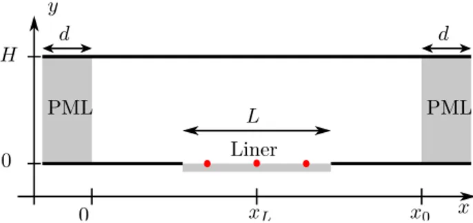
Fig. 1. Geometry of the lined flow duct. The three bullet points represent pressure sensors.
1.1. Governing equations and problem formulation
The configuration studied in this paper is a two-dimensional partially lined flow duct of height H. The length of the liner is denoted by L. The geometry is depicted in Fig. 1 together with the definitions of the coordinates system. The main flow (denoted with subscript 0) is purely in the axial direction (x-axis) and depends only on y. It is assumed to be subsonic, stationary and homentropic. Moreover, the main density ρ0and the sound speed a0are taken constant.
The Mach number of the main flow is denoted M0, its maximum value is denoted by M. In the following, all variables
are non-dimensionalized using the reference velocity, density, pressure, length and time Vre f = a0M, ρre f = ρ0,
pre f = ρre fVre f2 , lre f = L and tre f = lre f/Vre f, respectively.
We are interested by the evolution of a small perturbation, denoted ϕ, to this mean flow. This perturbation is taken under a general form ϕ(x, y, t) and is composed by the perturbation velocity vector u = uex+ veyand by the
perturbation pressure p: ϕ= (u, p). The evolution of this perturbation is governed by the linearised Euler equations in the domainΩ, written under a matrix form as (the Einstein summation is used on x and y):
∂tϕ + Aj∂jϕ + Bϕ = 0 (1)
At a wall (lined or not) is imposed an impedance boundary condition defined by Eq. (2) where Z is the specific impedance and n is the outward-pointing unit normal vector.
p= Zu · n (2)
No-slip boundary conditions are imposed on the main flow, which justifies the choice of Eq. (2) rather than a (en-hanced) Myers boundary condition as classically done when the main flow is supposed to be uniform16,17,18,19.
Inflow and outflow boundary conditions are dealt with by adding Perfectly Matched Layer (PML) absorbing lay-ers of width d to the computational domain (see Fig.1), as first proposed by B´erenger20 for computational electro-magnetics and then applied by Hu21 to aeroacoustics simulations. We follow his work to take special care on the absorbing capabilities of the PML layers in the presence of a mean flow.
Equations (1) are discretised in time by a Crank-Nicholson scheme, and in space by a discontinuous Galerkin method, the same as the one used by Pascal et al.22 to compute the eigenmodes in the transverse section of a lined
duct.
1.2. Optimal growth analysis
To study the amplifier dynamics of the configuration depicted in Fig. 1, a direct optimal growth analysis10 is
performed. We are interested in the computation of the initial perturbation ϕ0 = ϕ(t = 0) of energy E0 = E(t = 0)
which maximizes at the time horizon T the energy gain defined by G(T )= E(T)/E(0). In the current study, the energy is defined by: E(t)= h ϕ(t) ; ϕ(t) i Ω0 =Z Ω0 ϕ(t)2dΩ . (3)
The domainΩ0is the physical domain, i.e. the domain depicted in Fig. 1 without the PML layers. This energy, kinetic
swirling duct flow. It would have been as well possible to choose an energy corresponding exactly to the energy of a perturbation carried by a stationary base flow but it would have not been a conservative energy since the main flow is rotational24.
The Lagrangian multiplier technique is chosen to solve the optimization problem argmaxϕ0E(T ), with the added constraints that the governing equations (with PML) must be satisfied and the initial energy E0= h ϕ0; ϕ0i
Ω0
must be equal to 1. The stationarity of the Lagrangian yields especially to the conditions:
(i) ϕ∗(T )= 2ϕ(T) if x ∈ Ω0and ϕ∗(T )= 0 elsewhere;
(ii) ϕ0= ϕ0∗/||ϕ0∗|| if x ∈Ω0and ϕ0= 0 elsewhere.
where ϕ∗is the solution of the adjoint equations. It is worth noting that the discontinuous Galerkin formulation used in this paper offers the property of adjoint consistency, which means that the optimize-then-discretise and discretise-then-optimize strategies are equivalent. The optimize-then-discretise strategy is chosen here.
Finally, the optimization problem is solved by performing an iterative procedure in which both the direct and adjoint equations are integrated in time (forward and backward, respectively), with initial values provided by conditions (i) and (ii). At the end of the procedure, the optimal initial perturbation ϕ0for the time horizon T is obtained, as well as
the associated energy gain G(T ).
By repeating this procedure for every time horizon T , the optimal transient growth mechanism can thus be captured.
2. Numerical results
In the studied configuration, a Poiseuille flow defined by M0(y)= 4M(H − y)y/H2 is chosen, with M= 0.3. The
liner length is L = 4H and its impedance is Z = 10−2. This impedance is not representative of realistic liners, but it satisfies the four conditions given by Rienstra25 which ensure that an impedance model is physically realisable.
2.1. Local stability analysis
By assuming the liner of infinite length, local stability analysis is performed. The code developed by Brazier26,
previously used by Boyer et al.7, is used both for whole spectrum computation and eigenmodes tracking.
On Fig. 2 is plotted the spectrum obtained for ω = 11.8. In addition to acoustic modes and a continuous hy-drodynamic spectrum (associated to critical layer singularities), two discrete hyhy-drodynamic modes are found. By tracking the mode of wavenumber kHI≈ 24.5 − 7.8i while varying ω from 11.8 to 11.8+ 196i it is shown according to
the Briggs-Bers criterion (for further explanation, see Brambley18, Appendix A) that this is a convectively unstable right-running mode. By tracking its trajectory while ω is varied between 2 × 10⁻²and 196, it is found that ω= 11.8 is the real frequency that leads to the highest spatial growth rate. Moreover, when plotting the spectra obtained for ω = 2 × 10⁻²and ω = 196. (not shown here), it is observed that both at high and low frequencies the mode decays
into a mode of the continuous spectrum while in the computations of Boyer et al.7 the mode is originating at low
frequencies as an evanescent acoustic mode.
This configuration, though much more simplified than the experimental configuration of Aur´egan and Leroux4, is
therefore interesting to study hydrodynamic instabilities developing on acoustic lining. 2.2. Optimal growth
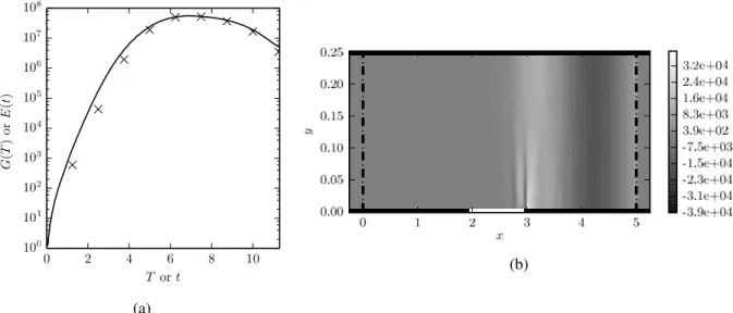
The time evolution of the optimal energy gain is plotted in Fig. 3(a). A transient growth is observed, and the optimal gain is maximized at Topt ≈ 7. The associated intial perturbation is denoted by ϕ0opt. It can be shown on
Fig. 3(a) (crosses) that the energy gain associated to this perturbation is close to the optimal gain whatever the time horizon, which means that ϕ0optis nearly optimal for all times.
It is worth noting that the maximum optimal gain G(Topt) is very high (≈ 5 × 10⁸), which can question the validity
of the linear assumption. The time-evolution of ϕ0optshows that this very large gain is associated to the radiation of a
Fig. 2. Spectrum obtained for ω = 11.8 (circles). The dashed and dotted lines represent the trajectories of the hydrodynamic mode obtained respectively for ω= 11.8 + [0 , 196]i and ω = [2 × 10⁻², 196] + 0i.
(a)
(b)
Fig. 3. (a) Energy gain versus the time horizon. The optimal gain is plotted in solid line. The crosses show the effective time-evolution gain of the optimal initial perturbation corresponding to the optimal time horizon Topt. (b) Spatial distribution of the optimal pressure perturbation at the
optimal time horizon. The lined section is displayed in white, the vertical thick dashed lines shows the boundaries of the PML layers.
pressure perturbation at the optimal time horizon Toptare plotted in Figs. 3(b) and 4. The two figures show the whole
spatial field and the spatial evolution along the bottom wall respectively.
2.2.1. Comparison with local stability analysis
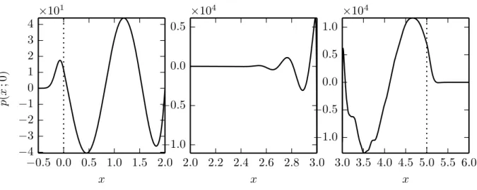
From the values and positions of the antinodes plotted Fig. 4, it is found that p(x, y= 0, t = Topt) (i.e. on the bottom
wall) behaves as a wave:
- of wavenumber k= 28.0 − 9.0i on the lined wall, - of wavelength λ−= 1.4 on the upstream rigid wall,
- of wavelength λ+= 2.2 on the downstream rigid wall.
The wavenumber found on the lined wall is close to kHI= 24.5 − 7.8i found in section 2.1. Moreover, a local stability
analysis performed for ω= 11.8 by considering both the upper and lower wall rigid gives two plane acoustic waves propagating downstream and upstream of wavelength 2.2 and 1.4 respectively.
Fig. 4. Spatial distribution of the optimal pressure perturbation at the optimal time horizon along the bottom wall (left: upstream rigid wall, middle: lined wall, right: downstream rigid wall. PML positions are given by the dashed vertical lines.
Fig. 5. Pressure measured on the liner at x= {xL− L/4, xL, xL+ L/4}.
In addition to the spatial evolution of the solution at t= Topt, the temporal behaviour is analysed by means of three
pressure sensors placed on the liner at x = {xL− L/4, xL, xL+ L/4} (and depicted Fig.1). On Fig. 5 are shown the
signals measured by propagating ϕopt0 . A wave packet amplified while travelling downstream is observed. A second wave packet is observed from t ≈ 6 on the first sensor and from t ≈ 8 on the second sensor, this will be discussed in section 3. The analysis of the three signals gives the angular frequency ω = 12.0 while the propagation speed of the envelope is 0.12. This frequency is close to the angular frequency ω = 11.8 found in section 2.1. Moreover the propagation speed of the envelope agrees reasonably well with the group velocity cg = 0.14 computed by local
stability analysis for ω= 11.8.
These spatial and temporal analyses confirm that the behaviour of the pressure field downstream of the liner Fig 3(b) corresponds indeed to the radiation of a plane acoustic wave of high amplitude as observed experimentally by Aur´egan and Leroux4. It shows moreover that the amplifier dynamics observed Fig 3(a) is closely linked to the hydrodynamic
instability found by a local approach. Finally, a plane acoustic wave travelling upstream is as well observed but is of much smaller amplitude than the right running plane acoustic wave.
(a)
(b)
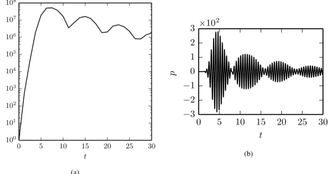
Fig. 6. (a) Time evolution gain of the optimal initial perturbation ϕopt0 . (b) Pressure measured on the liner at x= xL.
3. Stable/unstable resonances due to lining transition ?
On Fig. 5 was observed that a second wave packet was travelling downstream. In order to study more deeply this phenomenon, the initial perturbation ϕopt0 has been propagated from t= 0 to t = 30. On Fig.6(a) is shown the temporal behaviour of the energy. It is observed that rather than decaying quickly toward zero, the energy is slowly decreasing and oscillates. Moreover, as previously, the pressure has been measured on the liner at the same three positions. The three signals being qualitatively similar, only the pressure measured at x= xLis shown Fig.6(b). The signal looks like
a succession of decreasing wave-packets.
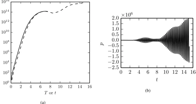
These results led us to believe that after a transient part, the evolution of the perturbation is driven by a pseudo-resonant mechanism. In order to further investigate the existence of a pseudo-resonant mechanism, a second non modal analysis has been performed with a liner of length L= 8H. The maximum gain has been computed for time horizons between T= 0 and T ≈ 7.5 and is plotted on Fig 7(a) (solid line). A first maximum of the optimal gain is observed at T = Topt= 6.5. The value of this maximum ≈ 1014is much higher than the maximum obtained with a liner of length
L = 4H. The initial perturbation leading to this maximum optimal gain is denoted ϕopt0 . A second computation has been performed by propagating the initial perturbation from t = 0 to t ≈ 15. On Fig 7 is shown the time-evolution of the perturbation energy (dashed line). This energy is close to the optimal gain, which shows that ϕopt0 is nearly optimal at least for all times between t = 0 and t = 7.5. Rather than decaying to zero, the perturbation is amplified again from t ≈ 9. On Fig.7(b) is shown the pressure signal measured on the liner at x= xL. This signal and the two
signals measured at x= xL− L/4 and x = xL+ L/4 (not shown here) show that after a transient stage characterised by
travelling wave-packets, an unstable harmonic regime is established.
These stable and unstable resonant behaviours could be due to a feedback mechanism between the unstable hydro-dynamic mode and the left-running evanescent mode k ≈ −1 − 5.3i (see Fig. 2), since the latter has a damping rate smaller than the amplification rate of the unstable hydrodynamic mode. For this reason, there might exist a critical length L for which the dynamics of the system switches from amplifier to resonator. Moreover, it may be supposed that this feedback mechanism could be the origin of the resonator dynamics reported by Pascal et al.27. In this paper (in
French), the authors have performed global modal analysis on a configuration similar to the configuration considered in the present study. They have found the existence of unstable temporal modes and have submitted the explanation
(a)
(b)
Fig. 7. Liner of length L= 8H. (a) Time evolution gain of the optimal initial perturbation ϕopt0 . (b) Pressure measured on the liner at x= xL.
that this resonator dynamics could be due to two-dimensional effects associated with hard-soft and soft-hard lining transition. The existence of a feedback mechanism associated to the reflections at lined/rigid transitions has been as well put forward by Marx28.
These (pseudo-)resonances are currently being deeply studied and will be the object of a future paper.
4. Conclusion
In this paper was performed a stability analysis in a lined flow duct where the lining is of finite extent. The considered geometry being therefore two-dimensional, global stability approach is followed. The study is performed in time-domain by searching the optimal initial condition maximising the energy of the perturbation at the time horizon T. Rather than considering the initial perturbation as a linear superposition of global modes, direct optimal growth analysis is chosen since it takes into account the full dynamics by considering the full linearised governing equations in time. This method consists in solving successively the direct and adjoint linearised Euler equations. The problem was discretised by means of discontinuous Galerkin method which offers the property of adjoint consistency. Finally, PML boundary conditions have been used to truncate the computational domain.
A Poiseuille flow is considered and the impedance of the liner has been chosen as constant and real. Although this configuration is not representative of realistic duct flow, it is appropriate to study hydrodynamic instability over a lined wall. As a matter of fact, when considering the liner of infinite extent, local linear stability analysis shows that a right-running hydrodynamic instability exists. It has been first shown that the amplifier dynamics, manifested by a transient growth, is closely related to the unstable hydrodynamic mode found by means of local stability theory. It has been shown, moreover, that this hydrodynamic instability is converted into a plane acoustic wave of high amplitude radiated downstream. In addition, an upstream-propagating plane acoustic wave of much smaller amplitude has been observed.
Finally, pseudo-resonant and resonant dynamics have been observed depending on the liner length. One hypoth-esis is that there is a feedback mechanism between the unstable right-running hydrodynamic instability and the less damped left-running acoustic mode which reflect at the leading and trailing edges of the liner. The understanding of this long-time behaviour requires further work.
References
1. Meyer, E., Mechel, F., Kurtze, G.. Experiments on the influence of flow on sound attenuation in absorbing ducts. The Journal of the Acoustical Society of America1958;30(3):165–174.
2. Brandes, M., Ronneberger, D.. Sound amplification in flow ducts lined with a periodic sequence of resonators. In: 1st AIAA/CEAS Aeroacoustics Conference; AIAA-95-126. 1995, p. 893–901.
3. J¨uschke, M.. Akustische Beeinflussung einer Instabilit¨at in Kan¨alen mit ¨uberstr¨omten Resonatoren. Ph.D. thesis; Nieders¨achsische Staats-und Universit¨atsbibliothek G¨ottingen; 2006.
4. Aur´egan, Y., Leroux, M.. Experimental evidence of an instability over an impedance wall in a duct with flow. Journal of Sound and Vibration2008;317(3):432–439.
5. Marx, D., Aur´egan, Y., Bailliet, H., Vali`ere, J.C.. PIV and LDV evidence of hydrodynamic instability over a liner in a duct with flow. Journal of Sound and Vibration2010;329(18):3798–3812.
6. Rienstra, S.. A classification of duct modes based on surface waves. Wave Motion 2003;37(2):119 – 135.
7. Boyer, G., Piot, E., Brazier, J.P.. Theoretical investigation of hydrodynamic surface mode in a lined duct with sheared flow and comparison with experiment. Journal of Sound and Vibration 2011;330(8):1793 – 1809.
8. Marx, D., Aur´egan, Y.. Comparison of experiments with stability analysis prediction in a lined flow duct. In: 16th AIAA/CEAS Aeroacoustics Conference; AIAA-2010-3946. 2010, p. 1–17.
9. Marx, D., Aurgan, Y.. Effect of turbulent eddy viscosity on the unstable surface mode above an acoustic liner. Journal of Sound and Vibration2013;.
10. Schmid, P.. Nonmodal stability theory. Annual Review of Fluid Mechanics 2007;39(1):129–162.
11. Barkley, D., Blackburn, H., Sherwin, S.. Direct optimal growth analysis for timesteppers. International journal for numerical methods in fluids2008;57(9):1435–1458.
12. Monokrousos, A., Åkervik, E., Brandt, L., Henningson, D.. Global three-dimensional optimal disturbances in the Blasius boundary-layer flow using time-steppers. Journal of Fluid Mechanics 2010;650:181.
13. Ehrenstein, U., Gallaire, F.. On two-dimensional temporal modes in spatially evolving open flows: the flat-plate boundary layer. Journal of Fluid Mechanics2005;536:209–218.
14. Sipp, D., Marquet, O.. Characterization of noise amplifiers with global singular modes: the case of the leading-edge flat-plate boundary layer. Theoretical and Computational Fluid Dynamics 2012;:1–19.
15. Marquet, O., Sipp, D., Chomaz, J.M., Jacquin, L.. Amplifier and resonator dynamics of a low-reynolds-number recirculation bubble in a global framework. Journal of Fluids Mechanics 2008;605:429–443.
16. Ingard, U.. Influence of fluid motion past a plane boundary on sound reflection, absorption, and transmission. The Journal of the Acoustical Society of America1959;31(7):1035–1036.
17. Myers, M.. On the acoustic boundary condition in the presence of flow. Journal of Sound and Vibration 1980;71(3):429–434.
18. Brambley, E.J.. Fundamental problems with the model of uniform flow over acoustic linings. Journal of Sound Vibration 2009;322:1026– 1037.
19. Brambley, E.. A well-posed boundary condition for acoustic liners in straight ducts with flow. AIAA Journal 2011;49(6):1272–1282. 20. B´erenger, J.P.. A perfectly matched layer for the absorption of electromagnetic waves. Journal of Computational Physics 1994;114(2):185
– 200.
21. Hu, F.. A perfectly matched layer absorbing boundary condition for linearized Euler equations with a non-uniform mean flow. Journal of Computational Physics2005;208(2):469 – 492.
22. Pascal, L., Piot, E., Casalis, G.. Discontinuous Galerkin method for the computation of acoustic modes in lined flow ducts with rigid splices. Journal of Sound and Vibration 2013;332(13):3270 – 3288.
23. Cooper, A.J., Peake, N.. Transient growth and rotor-stator interaction noise in mean swirling duct flow. Journal of Sound and Vibration 2006;295(3-5):553–570.
24. Myers, M.. Transport of energy by disturbances in arbitrary steady flows. Journal of Fluid Mechanics 1991;226:383–400.
25. Rienstra, S.W.. Impedance models in time domain, including the extended Helmholtz resonator model. In: 12th AIAA/CEAS Aeroacoustics Conference; AIAA-2006-2686. 2006, p. 1–20.
26. Brazier, J.P.. MAMOUT : Module d’analyse modale unidimensionnelle avec les polynmes de Tchebychev. Instructions pour l’emploi des programmes SPECTRE et MODITER version 5. Tech. Rep.; Onera; 2011.
27. Pascal, L., Piot, E., Casalis, G.. Analyse de stabilit´e globale et instabilit´e hydrodynamique dans un conduit trait´e acoustiquement. In: CFA 2014 Poitiers. 2014, p. 617–623.
28. Marx, D.. Numerical simulation of physical instabilities in a lined channel using the linearized euler equations. In: CFA 2014 Poitiers. 2014, p. 583–589.