Spatial spin-up of fine scales in a regional climate model simulation driven by low-resolution boundary conditions

DOI 10.1007/s00382-016-3358-2

Spatial spin‑up of fine scales in a regional climate model

simulation driven by low‑resolution boundary conditions

Received: 29 April 2016 / Accepted: 7 September 2016

© The Author(s) 2016. This article is published with open access at Springerlink.com

corresponds to a fixed number of RCM grid points that is a function of resolution jump only. These findings can serve a useful purpose to guide the choice of domain and RCM configuration for an optimal development of the small scales allowed by the increased resolution of the nested model.

Keywords Regional climate modelling · Nested model ·

Jump of resolution · Spatial spin-up · Big-Brother experiment

1 Introduction

Climate models are useful tools to understand past, pre-sent and future climate conditions. Coupled global climate models (CGCM) are designed to represent the atmosphere, ocean, cryosphere and land surfaces and their interac-tions. To simulate the climate in a reasonable time, a large number of simplifying assumptions are made, and several processes are simply parameterised to reduce the computa-tional cost. Nevertheless, achieving resolutions required by several impact studies would drastically increase the com-putational cost, which would exceed the limits of available computing infrastructure. To overcome this issue, the use of regional climate models (RCM) has become a pragmatic avenue to achieve high-resolution climate simulations at an affordable computational cost. RCM are limited-area mod-els, one-way nested at their lateral boundaries by low-reso-lution CGCM-simulated or reanalyses data.

CGCM spatial resolution has changed little over the last decade. The average grid mesh of CGCM participating in century-long IPCC AR5 climate projections was about 321 km (equivalent to ≈T62 using the linear transform grid spacing for spectral models). Whereas RCM grid meshes

Abstract In regional climate modelling, it is well known

that domains should be neither too large to avoid a large departure from the driving data, nor too small to provide a sufficient distance from the lateral inflow boundary to allow the full development of the small-scale (SS) features permitted by the finer resolution. Although most practition-ers of dynamical downscaling are well aware that the jump of resolution between the lateral boundary condition (LBC) driving data and the nested regional climate model affects the simulated climate, this issue has not been fully inves-tigated. In principle, as the jump of resolution becomes larger, the region of interest in the limited-area domain should be located further away from the lateral inflow boundary to allow the full development of the SS features. A careless choice of domain might result in a suboptimal use of the full finer resolution potential to develop fine-scale features. To address this issue, regional climate model (RCM) simulations using various resolution driving data are compared following the perfect-prognostic Big-Brother protocol. Several experiments were carried out to evaluate the width of the spin-up region (i.e. the distance between the lateral inflow boundary and the domain of interest required for the full development of SS transient eddies) as a function of the RCM and LBC resolutions, as well as the resolution jump. The spin-up distance turns out to be a function of the LBC resolution only, independent of the RCM resolution. When varying the RCM resolution for a given resolution jump, it is found that the spin-up distance

* Dominic Matte

mattedominic3@gmail.com

1 _{Department of Earth and Atmospheric science, Centre}

ESCER, Université du Québec à Montréal (UQAM), P.O. Box 8888, Downtown Station, Montréal, QC H3C 3P8, Canada

remained mainly unchanged at 45–60 km for the initial two decades, they have been refined to 10–15 km in the last decade (e.g. EURO-CORDEX, Vautard et al. 2013; Jacob et al. 2014) and have recently reached convection-permit-ting values of 2.5–4 km (e.g. Pan et al. 2011; Rasmussen et al. 2014; Fosser et al. 2014; Ban et al. 2015). The dis-parity of resolution between increasingly high-resolution RCM and lateral boundary conditions (LBC) provided by low-resolution CGCM raises important issues, such as the dynamical equilibrium between the inner solution calcu-lated by the RCM and the outer solution provided by LBC, the different formulations and/or prognostic variables in LBC and RCM, and the spatial spin-up. The latter issue is the focus of this paper.

Spatial spin-up is the phenomenon by which small-scale (SS) features that are absent in the driving LBC develop as permitted by the higher spatial resolution of the nested model. Previous studies (Leduc and Laprise 2009; Leduc et al. 2011) have shown that a minimum domain size is required for the SS to develop and reach their full potential. These studies showed that for a jump of resolution between the LBC and the nested model of 12 (roughly equivalent to a T30 spectral model driving a 45 km RCM), a domain size of 144 × 144 grid points was barely sufficient for the SS to fully develop in the low levels in summer, and even larger domain sizes were required to reach a full develop-ment aloft and in winter due to stronger flow through the domain. With a resolution jump of six, Colin et al. (2010) and Køltzow et al. (2011) noted that precipitation was underestimated near the western (inflow) boundary of their domain, a likely manifestation of spatial spin-up. Brisson et al. (2015) noted some deficiencies in their convection-permitting climate simulations when using single nesting, likely as a result of a large resolution jump combined with large nesting time intervals. Matte et al. (2016) have shown that the use of multiple nesting reduces the resolution jump, with a positive impact on the SS development.

The focus of this study is on characterizing the impact of the resolution jump on SS spin-up in RCM simulations, by analysing the spatial development of SS from the lat-eral boundaries through the RCM domain, rather than the effect of domain size as in previous studies. The sought outcome of this study is the determination of the “trust-worthy” region within an RCM domain, trustworthy in the sense that SS permitted by the high resolution have reached their asymptotic amplitude. The idealised Big-Brother experimental protocol will be used to address this issue. This paper is organized as follows. A brief description of the regional model followed by a description of the experi-mental design are presented in Sect. 2. The results are detailed in Sect. 3. Finally, Sect. 4 summarises the findings and concludes.

2 Experimental design

The experiments have been performed with the fifth-gener-ation Canadian RCM (CRCM5; see Hernández-Díaz et al.

2013 for a detailed description). The physical parameteri-zation of the CRCM5 is mostly based on the 33-km meso-global GEM model (Bélair et al. 2005, 2009) employed for numerical weather prediction by the Canadian Mete-orological Centre (CMC). The model configuration uses Kain-Fritsch deep convection parameterization (Kain and Fritsch 1990), Kuo-transient shallow convection (Kuo

1965; Bélair et al. 2005), Sundqvist resolved-scale con-densation (Sundqvist et al. 1989), correlated-K terrestrial and solar radiation schemes (Li and Barker 2005), subgrid-scale orographic effects are parameterized following the McFarlane mountain gravity-wave drag (McFarlane 1987) and the low-level orographic blocking scheme of Zadra et al. (2003), and turbulent kinetic energy closure planetary boundary layer and vertical diffusion (Benoit et al. 1989; Delage and Girard 1992; Delage 1997). Unlike the NWP version of GEM however, CRCM5 uses the most recent version of the Canadian Land Surface Scheme (CLASS 3.5; Verseghy 2000, 2008) that allows a detailed represen-tation of vegerepresen-tation, land-surface types, organic soil and a flexible number of layers, and lakes are represented by the 1-D FLake model (Martynov et al. 2012). In the vertical, 56 levels are used.

To investigate the impact of the driving data resolution upon the development of SS features in a high-resolution RCM, the Big-Brother Experiment (BBE) protocol, origi-nally designed by Denis et al. (2002b) is used. This experi-ment employs a perfect prognosis approach that isolates the nesting errors from other modelling errors, thus emphasiz-ing the influence of nestemphasiz-ing on the RCM solution. In the BBE, a first simulation named the Big Brother (BB) is realized on the largest possible domain. The BB simula-tion serves two purposes: (1) it is used as a reference to evaluate the test simulations nicknamed the Little-Brother (LB) simulations, and (2) it provides, after filtering, initial and driving lateral boundary conditions for LB simula-tions that are performed using the same model formulation and resolution as the BB. The BB data are processed by a low-pass filter to mimic the low-resolution GCM driv-ing data. The resultdriv-ing filtered BB datasets will be noted BB_Fr, with r the equivalent mesh size resolution. These BB_Fr fields are, in some sense, perfect as far as the large scales are concerned, because they do not suffer from sim-ulation errors that would have occurred in coarse-mesh model simulations. However, the BB_Fr fields are devoid of SS as coarse-mesh GCM simulations would be. The LB-simulated SS can be compared with those of the verifying BB to assess the dynamical downscaling skill of various

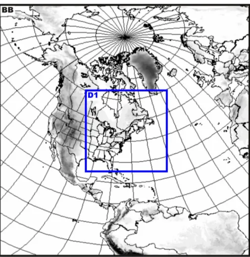
configurations of LBs and resolution jump by varying BB_ Fr. Shown in Fig. 1, the CRCM5 simulation on a 0.15° mesh (roughly 17 km) covering a 760 × 760 grid-point free domain centred on Montréal, Québec, Canada, served as BB. The BB simulation is driven by the ERA-Interim reanalysis for eight 2-month long periods, starting on June 1st for summer and November 1st for winter, of the years 1997, 1998, 1999 and 2000. For these simulations the time step is 5 min. The BB simulation is driven by ERA-Interim data available at 6-hourly intervals.

Low-resolution LBC were generated by applying a low-pass filter based on the discrete cosine transform (DCT: Denis et al. 2002a), with a gradual response function that attempts to mimic the spectrum of equivalent grid-mesh simulations. The lower and upper limits were chosen to correspond, respectively, to the Nyquist length scale 2 ∆ x and to the smallest adequately resolved scales 7 ∆x, as shown by Skamarock (2004) and Cholette et al. (2015), with a cosine-squared function transition between these two values. LBC corresponding to three resolution jumps (J) were generated. For J = 24, corresponding to a mesh of 3.6° (noted as BB_F3.6), the lower and upper wavelength limits were chosen to be 792 and 2772 km; for J = 12, cor-responding to a mesh of 1.8° (noted as BB_F1.8), the limits

were 396 and 1386 km; and for J = 3, corresponding to a mesh of 0.45° (noted as BB_F0.45), the limits were 100 and 346 km. The LB simulations were performed for 1.5-month periods starting on November 15 for winter and on June 15 for summer (thus leaving out the initial 15 days as spin-up of the BB simulation), for the years 1997 to 2000, using the BB_Fr dataset as IC and LBC (geopoten-tial height, temperature, zonal and meridional winds, spe-cific humidity and water content) at 1-hourly intervals. The LB simulations were performed on a free domain of 260 × 260 grid points (noted as D1 in Fig. 1), surrounding by the Davies zone of 10 grid points which is weighted by a cosine-squared function. Unlike previous studies dealing with spatial spin-up with different domain sizes, here we used a rather large LB domain to ensure that SS amplitudes could develop to their asymptotic value within the domain. The climate statistics of the LB simulations will be com-pared to those of the BB for the four months of December and July, thus leaving out the initial 15 days as temporal spin-up of the LB simulations. Four sets of LB simulations will be performed; three of them will be nested with data-sets BB_F3.6, BB_F1.8 and BB_F0.45, noted as LB_J24, LB_J12 and LB_J3, corresponding to resolution jumps of 24, 12 and 3, respectively, and a fourth one driven directly

Fig. 1 The domain of the

Big-Brother simulation (BB) (free domain of 760 × 760 grid points). All the Little-Brother simulations have a free domain of 260 × 260 grid points centred on Montréal (D1)

by BB, noted LB_J1, corresponding to a resolution jump of 1.

3 Results

In the analysis, fine-scale transient eddies in LB simula-tions driven by various BB_Fr will be compared with those of the reference BB. The departure of the time-mean com-ponents (also called transient-eddy component) will be ana-lyzed. Any variable Ψ (x, t), function of space x and time t, will be decomposed as follows

where • is the temporal mean and ’ the time deviation. The transient-eddy standard deviation is obtained as

A DCT filter is employed to isolate the SS from the total field. The DCT filter was configured to eliminate wave-lengths larger than 400 km and retain those smaller than 300 km, with a gradual cosine-squared function transition in between. As defined, the SS that are analyzed in LB_J24 and LB_J12 were completely absent of the driving LBC and developed within the LB simulations. However, for LB_J3, the limits of the DCT filter used to produce LB_J3 and the SS field slightly overlap. Thus, a small part of the SS (those with wavelengths in the range 300–346 km) are present in the driving data for this case; nevertheless, the SS spin-up process can still be observed in LB_J3.

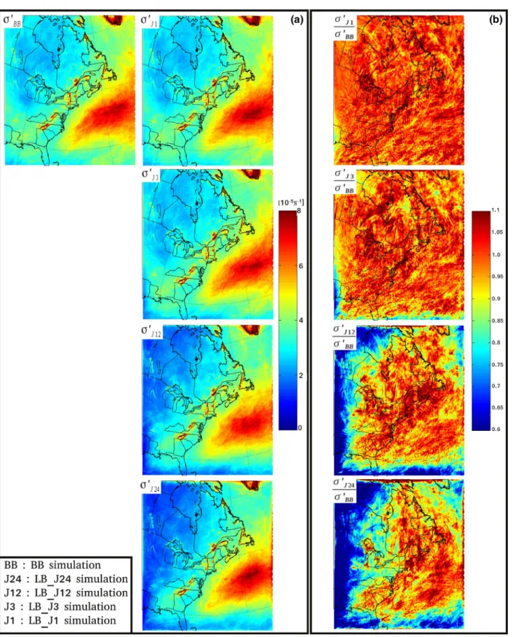
Figure 2 illustrates the SS spatial spin-up for differ-ent jumps of resolution for the 700-hPa relative vorticity in December; this variable is chosen for its abundant SS features. Figure 2a presents maps of the standard devia-tion of the SS transient-eddy component for the BB and the four LB_Ji simulations, called σ′

BB and σ ′

Ji,

respec-tively, on the free LB domain (see D1 domain in Fig. 1). In the BB, large values are noted on the East Coast, corresponding to the North Atlantic storm track at this period of the year. Some spotty large values are also seen over the Appalachians due to orographic effects. On the flat continent, relatively smooth small values are noted almost everywhere. In the LB_Ji simulations, weaker val-ues can be seen at the western and southern edges of the domain, more pronounced for larger resolution jumps; these smaller values reflect the underdeveloped SS fea-tures downstream of the inflow boundaries, with the dom-inant westerly flow in winter. Spatial spin-up becomes even clearer by looking at the σ′

Ji normalized by the

refer-ence value σ′

BB as shown in Fig. 2b. The red colour

corre-sponds to values near unity, hence confirming the devel-opment of the SS features to their asymptotic amplitude.

(1) Ψ (x, t) = Ψ (x) + Ψ′(x, t) (2) σ′ (x) =  Ψ′2_(x)

The underestimation of the SS transient-eddy amplitude near the boundary inflow of the domain is clearly vis-ible, especially for the largest resolution jumps. Clearly, results in the spin-up zone should be taken cautiously because the fast atmospheric flow has not yet developed the SS permitted by the fine mesh.

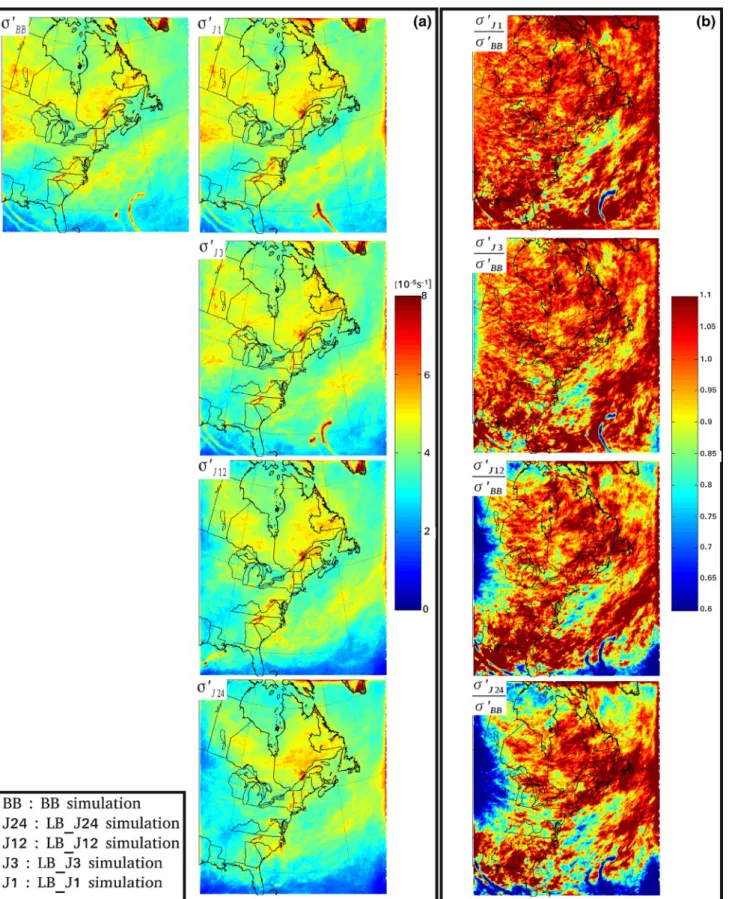
Figure 3 shows the corresponding results in July. Over-all, the results in summer are similar than in winter, except that the spin-up zones at the western and southern edges of the domain are narrower due to the weaker general atmos-pheric circulation in summer than in winter, as noted before by Leduc et al. (2011).

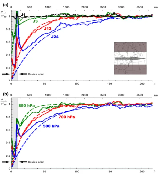
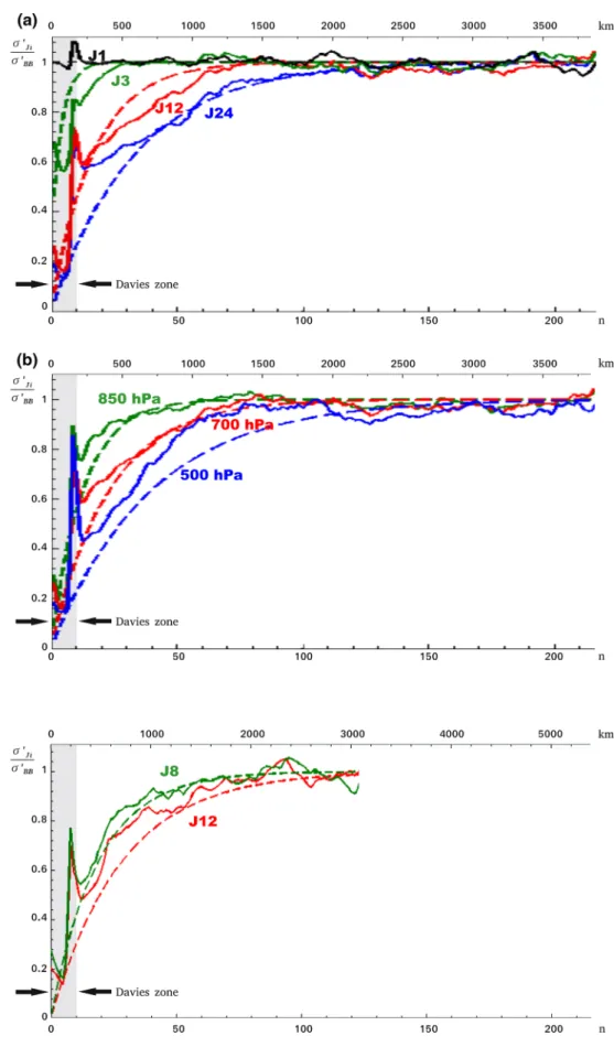
Figures 4 and 5 show the value of the ratio σJi′ σ′

BB

 along a West-to-East cut, across the domain, for different jump of resolution J, for the 700-hPa relative vorticity SS transient-eddy standard deviation averaged over the middle third of the domain (indicated at the bottom right of Fig. 4a, for December and July, respectively. This West to East section of the domain is used as it corresponds to the mean atmos-pheric flow for this region. The lower abscissa corresponds to the distance from the western boundary expressed in number of grid points (n) and the upper abscissa corre-spond to the distance expressed in km. Figures 4a and 5a show the gradual increase of the ratio towards unity with increasing distance from the western boundary. It can be noted that the distance required to approaching the full development of the SS increases with the resolution jump. Hence, when large jump of resolutions are considered, large domains are required to achieve the full development of the SS features permitted by the resolution of the driven model, as noted before by Leduc and Laprise (2009) and Leduc et al. (2011). Figures 4b and 5b show the ratio σJi′

σ′

BB

for the relative vorticity at different levels for the J12 case. It can be seen that the SS spin-up distance increases in the vertical, likely related to faster wind speed in the upper levels.

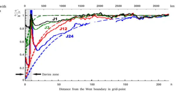
Figure 6 shows the result obtained in a similar experi-ment configured as previously for December, but with a grid mesh of 0.45° rather than 0.15° for J8 and J12. By comparing this J12 result with the corresponding J12 case with 0.15° shown in Fig. 4, it becomes clear that the spin-up distance varies in proportion to the RCM grid mesh in such a way that it covers the same number of grid points. This indicates that when varying the RCM resolution for a given resolution jump (hence varying the LBC resolution in proportion to the RCM resolution), the spin-up distance is best measured in terms of number of grid points rather than physical distance. On the other hand, when comparing the results obtained for J8 with a grid mesh of 0.45° shown in Fig. 6 with those obtained for J24 with a grid mesh of 0.15° shown in Fig. 4 (note that the LBC resolutions are the same in these two cases), the physical distance of spin-up are the same.

Fig. 2 a Small-scale transient-eddy standard deviation of the 700-hPa relative vorticity for the four December simulations. b Ratios of the LB

simulations standard deviation with that of the reference BB simulation σJi′ σ′

BB 

The experimental results shown in Figs. 4, 5 and 6 sug-gests a parametric curve for the spatial variation of SS tran-sient eddies of the form

where x is the distance from the lateral sponge zone (when expressed in terms of grid points, x = n∆xRCM, where n

is the number of grid points whithin the RCM domain), L is the e-folding distance on which the asymptotic value is reached (in terms of grid points, L = N∆xR, where N is a

e-folding distance in grid points ), and 0 ≥ k ≤ 1 a parameter to account for possible overlap between the definition of the SS in the driving data and the RCM (k = 1 for no overlap and k = 0 for full overlap). Such form makes some intui-tive sense: SS eddies that are absent in the LBC develop on the RCM high-resolution grid, as a result of various forc-ings (local physiographic, diabatic, nonlinear interactions, hydrodynamic instabilities, etc.), gradually increasing

(3) σ′ Ji σ′ BB (x) = 1 − k exp −x L 

in amplitude towards their asymptotic value within the domain. The results presented in Figs. 4 and 5 covered sev-eral variations of RCM grid meshes (∆xRCM), LBC

resolu-tion (∆xLBC) and resolution jump (J = _∆x∆xLBC

RCM). The

follow-ing dependencies can be deducted from these results: • L increases with height in the troposphere; closer

analy-sis revealed that L varies with the average wind speed V through the domain at the level of the variable that is analysed: L∝V.

• L varies with the shortest scale resolved by the LBC data: L∝2∆xLBC

This suggests writing

When ∆xRCM is held fixed and recalling the definition

pre-viously mentionned of L, Eq. (4) can be written as

(4) L = 2∆xLBCV

C .

Fig. 4 a West to East cut,

across the domain, (as shown at the bottom right of panel a) of the small-scale transient-eddy standard deviation for the rela-tive vorticity at 700 hPa of LB_ Ji normalized by the reference simulation BB, as a function of the distance from the western boundary (in km and number of grid points (n) in the upper and lower abscissa respectively in

both panel), for the four months of December. The different jumps of resolution J24, J12, J3 and J1 are shown by the

blue, red, green and black lines, respectively. b Same as a but only for J12 at three different levels: 850 hPa (green), 700 hPa (red) and 500 hPa (blue).The empirical Eqs. (6) and (7) are indicated by the dashed lines

Fig. 5 Same as Fig. 4 but the four July months

Fig. 6 Equivalent to Fig. 4a, but for similar experiment real-ized with an RCM on a 0.45° mesh rather than 0.15° mesh

where C is a constant with units of speed for dimensional consistency. The optimum fit with the experimental results led to the value C = 9 m s−1_{, which happens to correspond}

roughly to the typical displacement speed of synoptic-scale weather systems and to the ratio of their length and time scales (Orlanski 1975).

So, using Eq. (4), Eq. (3) becomes

while using Eq. (5), Eq. (3) than becomes

The optimum fit was obtained by setting the empirical con-stant k to 1 for J24 and J12, to 0.7 for J3 and to 0 for J1, to reflect the overlap in the definition of SS in the experiments as carried out. Eqs. (6) and (7) indicate that the adjust-ment distance is measured in terms of grid point numbers rather than physical distance when ∆xRCM is held fixed and

∆xLBC varies, while the adjustment distance is measured in

terms of physical distance when ∆xLBC is held fixed and

∆xRCM varies. Those two equations are indicated by the

dashed lines in Figs. 4, 5 and 6.

(5) N = 2JV C . (6) σ_Ji′ σ′ BB (x) =1 − k exp  _−xC 2∆xLBCV  , (7) σ_Ji′ σ′ BB (x = n∆xRCM) =1 − k exp  −nC 2JV  .

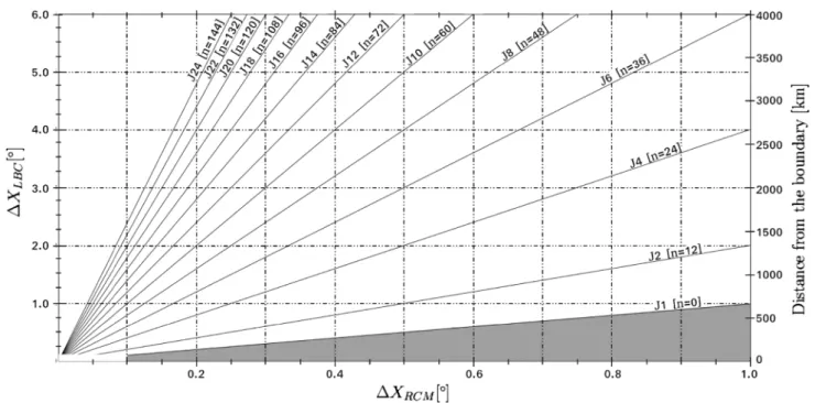
Figure 7 illustrates the equations and can serve as an abacus to evaluate the domain required to obtain the full development of the SS for a given set of available LBC and RCM resolution. The figure shows the values of the dis-tance 3 L (right hand y-axis) and 3 N (solid black lines) required to attain 95 % of the asymptotic amplitude of SS. The left hand y-axis is the grid mesh of the LBC and the abscissa is the grid mesh of the RCM. Practitioners have to look at the intersection of the grid mesh of the LBC and the RCM of the wanted simulation to know the distance (in number of grid point or in physical distance, depending on the point of view) to correctly develop the small-scale features.

4 Conclusion

This study investigated the spatial spin-up distance as a function of the jump of resolution using the idealised Big-Brother protocol. A Big-Big-Brother (BB) simulation was first performed with the CRCM5 on a 0.15° mesh over a very large domain over eastern North America, for two winter and two summer months of 4 years, driven by ERA-Interim reanalysis data. Then, this simulation was filtered to pro-duce fields with a resolution equivalent to 3.6°, 1.8° and 0.45° meshes. The resulting dataset were used to drive a series of Little-Brother (LB) simulations, with a resolution

Fig. 7 An abacus developed from Eqs. (6) and (7) showing the dis-tance 3 L (right hand y-axis) and 3 N (solid black lines) required to attain 95 % of the asymptotic amplitude of the small-scale transient

eddies, as a function of the grid mesh of the LBC (ordinate) and RCM (abscissa), respectively, for an average wind speed V equal to the typical speed of synoptic-scale weather systems C (V≈C)

jump of 24, 12 and 3, respectively, between the driving lateral boundary conditions and the LB mesh. An addi-tional experiment with a jump of resolution of 1 was also made. Some limited experiments were also carried out with CRCM5 simulations on a 0.45° mesh.

Throughout this paper, the behaviour of small-scale transient eddies was studied using the relative vorticity field because this variable is typical of atmospheric vari-ables that exhibit substantial small-scale amplitude, similar to vertical velocity or specific humidity, but unlike vari-ables such as geopotential height whose spectrum is dom-inated by larger scales. It is worth noting that other vari-ables have also been analysed but were not shown (such as meridional and zonal wind components, relative humidity), and conclusions remain the same. The 700-hPa level was chosen because it is close to the steering level of mid-lati-tude weather systems, near the level of non-divergence and maximum vertical velocity, and hence where precipitation is generated. In principle, this analysis could be extended to any variable and height of specific interest for some appli-cation of RCM simulations.

It has been shown that small-scale features take a large distance to develop within the simulated domain for large jump of resolution, particularly in winter and in the upper levels where the average flow through the domain is faster. It was found that the results could be summarized with a parametric equation describing the variation of the SS tran-sient-eddy amplitude from the inflow boundary, and hence the spin-up distance.

Our initial preconception was that the spin-up distance would increase with the resolution jump between the LBC and the RCM resolutions. The results obtained with the ide-alised BBE have shown however that the spin-up distance that scales with the resolution jump is not the physical dis-tance but rather the disdis-tance as measured in terms of RCM grid point numbers (see Eq. 7). For a given set of LBC, its resolution alone determines the spin-up physical distance, independently of the RCM resolution; hence when vary-ing the RCM resolution for a given set of LBC, the number of RCM grid points over which SS approach their asymp-totic value increases linearly with the resolution jump (see Eq. 6).

This parametric equation may be useful to RCM prac-titioners to determine an optimal domain to ensure the full development of the SS permitted by the resolution of the RCM used. The potentially trustworthy region of the RCM domain must exclude the spin-up region where fine scales have not yet reached their mature amplitude, thus shedding doubt on the simulated results in this region. Furthermore, RCM practitioners of the multiple nesting approach should also be aware of the location of the trustworthy region of each of their intermediate spatial-resolution simulation for an optimal used of this approach.

The fact that those results were provided from a 1-h nesting interval simulation might rise some questions about spatial spin-up at a more relaxed nesting interval. In fact, it can be demonstrated that the nesting time interval should be related to the resolution jump. For more detailed description, we referred the reader to the “Appendix”. A related point to also consider is the sensitivity to the width of the boundary relaxation zone. It is worth noting that this point has been assessed in another study, not reported in this paper. In essence the results have shown that the width of the blending zone has little effect upon the fine scales, its effect being felt mainly in the large scales that are better reproduced when expanding the blending zone.

Hence, in the interpretation of RCM simulations, it is important to take into account the small-scale spin-up region and exclude it from the analysis. In the last decade, several efforts have been made to foster high-resolution cli-mate-change information through coordinated experiments such as CORDEX in which a strict simulation framework is imposed, including domain size and location. The results in this study suggest that the spatial spin-up should be taken into account in the design of the simulation framework and the ensuing analysis to avoid that spatial spin-up might con-taminate results over the region of interest. Finally, further studies are needed for different domains location to vali-date the main conclusion of this study. However, the wind dependency of the empirical law suggests a strong relation between the weather regime and the small-scale develop-ment, which might give a good insight of how small scales are developed for other domains where the general weather regime is well known.

Acknowledgments This research was supported by the Natural

Sciences and Engineering Research Council (NSERC) of Canada. Computations were made on the supercomputer guillimin, managed by Calcul Québec and Compute Canada. The operation of this super-computer is funded by the Canada Foundation for Innovation (CFI), the Fonds de recherche du Québec—Nature et technologies (FRQNT), NanoQuébec, and the Réseau de médecine génétique appliquée (RMGA). D.M. thanks the FRQNT for a graduate fellowship. The authors are greatly indebted to Dr. Ramón de Elía for his construc-tive comments, to Dr. Bernard Dugas and Ms. Katja Winger for their essential help with the use of CRCM5, and to Mr. Georges Huard and Ms. Nadjet Labassi for maintaining user-friendly local computing facilities.

Appendix: Spatial spin‑up and nesting interval Figure 8 shows the same results as Fig. 4a, except that the nesting interval is extended to 6-hourly instead of hourly. To compare with the previous case, Eqs. (6) or (7) has also been used to draw the parametric curves computed in Fig. 8

for each Ji, showing clear differences with results when the nesting interval was set to 1 h. For the two larger jumps

of resolution (i.e. J24 and J12), no difference is noted with respect to Fig. 4a. However, J3 and J1 struggle more to fulfill the σJi′

σ′

BB

deficit due to the excessively long nesting interval. This means that even when all scales are provided by the driving data, a excessively long nesting interval degrades the development of small-scale features, which has also been noted in previous studies (McDonald 2005,

2006; Termonia et al. 2009; Omrani et al. 2012). It will be demonstrated below that the nesting time interval should be related to the resolution jump.

Consider a weather disturbance in the nesting data used to provide the LBC to drive an RCM. For simplicity we will assume a sinusoidal shape in one dimension, with wavenumber κ = 2π

, wavelength , moving at phase speed

C:

In practice, the nesting data is only available at discrete time intervals tn, with n an integer, and hence it needs to be

inter-polated in time between nesting intervals τ = tn+1−tn to

drive the RCM at each time step. For most RCM applica-tions, linear interpolation is used between nesting intervals to obtain values at intermediate times. Consider the interpo-lated value at the middle time between two nesting intervals:

Trigonometric identities give the result

Recognising the exact solution as Asinκ(x − C(tn+τ/2)),

the factor r = cosκCτ/2 appears as the numerical response of the linear interpolation. This factor may be written as (8) Ψ (x, tn) = Asinκ(x − Ctn) (9) Ψ (x, tn+1/2) ≈ Ψ (x, tn) + Ψ (x, tn+1) 2 (10) Ψ (x, tn+1/2) ≈ A 2(sinκ(x − Ctn) +sinκ(x − C(tn+τ ))) =Asinκ(x − C(tn+τ/2))cosκCτ/2

r = cosπ δ/ where δ = Cτ is the displacement distance of the disturbance in between two nesting time intervals. The interpolation provides an excellent approximation when δ ≪  (i.e. τ → 0) because factor r → 1 as expected; but the results degrade for larger displacement and in fact r = 0 for δ/ = 1/2. To obtain acceptable results, one should hence aim for values of f ≡ δ/ definitely smaller than a half. The shortest length scales for  are limited by reso-lution of the nesting data. Considering that LBC are pro-vided by a driving model with grid mesh ∆xLBC, then

 ≥ N∆xLBC where 2 ≤ N ≤ 7; N = 2 corresponds to

the Nyquist cut-off and corresponds approximately to the shortest well resolved scales (e.g. Skamarock 2004). Con-sider a resolution jump J = ∆xLBC

∆xRCM between the resolution of

the driving data and the RCM, we can then write

or

for the largest acceptable nesting time interval. Using parameter values f = 1/5, N = 7, C = 30 km h−1 _and

∆xRCM =20 km, we get τ ≈ Jh. This empirical equation

confirms the results shown in Fig. 8 showing that, for an RCM with ∆xRCM=20 km, a nesting interval of 6 h is

adequate for J equal to 12 and 24, but not for J equal to 1 and 3, in which case τ = 1h is adequate.

Open Access This article is distributed under the terms of the

Crea-tive Commons Attribution 4.0 International License (

http://crea-tivecommons.org/licenses/by/4.0/), which permits unrestricted use,

distribution, and reproduction in any medium, provided you give appropriate credit to the original author(s) and the source, provide a link to the Creative Commons license, and indicate if changes were made. (11) f = δ  = Cτ N ∆xLBC = Cτ NJ∆xRCM (12) τ = fNJ∆xRCMC

Fig. 8 Same as Fig. 4a but with a nesting time interval of 6 h

References

Ban N, Schmidli J, Schär C (2015) Heavy precipitation in a chang-ing climate: does short-term summer precipitation increase faster? Geophys Res Lett 42(4):1165–1172. doi:10.1002/201 4GL062588

Bélair S, Mailhot J, Girard C, Vaillancourt PA (2005) Bound-ary layer and shallow cumulus clouds in a medium-range forecast of a large-scale weather system. Mon Weather Rev 133(7):1938–1960

Bélair S, Roch M, Leduc AM, Vaillancourt PA, Laroche S, Mailhot J (2009) Medium-range quantitative precipitation forecasts from Canada’s new 33-km deterministic global operational system. Weather Forecast 24(3):690–708

Benoit R, Côté J, Mailhot J (1989) Inclusion of a TKE boundary layer parameterization in the Canadian regional finite-element model. Mon Weather Rev 117(8):1726–1750

Brisson E, Demuzere M, van Lipzig NP (2015) Modelling strategies for performing convection-permitting climate simulations. Mete-orl Z. doi:10.1127/metz/2015/0598

Cholette M, Laprise, Thériault JM (2015) Perspectives for very high-resolution climate simulations with nested models: Illustration of potential in simulating St. Lawrence River valley channel-ling winds with the fifth-generation Canadian Regional Climate Model. Climate 3(2):283–307. doi:10.3390/cli3020283

Colin J, Déqué M, Radu R, Somot S (2010) Sensitivity study of heavy precipitation in limited area model climate simulations: influence of the size of the domain and the use of the spectral nudging technique. Tellus A 62(5):591–604

Delage Y, Girard C (1992) Stability functions correct at the free con-vection limit and consistent for both the surface and Ekman lay-ers. Bound Layer Meteorl 58(1–2):19–31

Delage YAA (1997) Parameterising sub-grid scale vertical transport in atmospheric models under statically stable conditions. Bound Layer Meteorl 82(1):23–48

Denis B, Côté J, Laprise R (2002a) Spectral decomposition of two-dimensional atmospheric fields on limited-area domains using the discrete cosine transform (DCT). Mon Weather Rev 130(7):1812– 1829. doi:10.1175/1520-0493(2002)130<1812:SDOTDA>2.0.CO;2

Denis B, Laprise R, Caya D, Côté J (2002b) Downscaling ability of one-way nested regional climate models: the Big-Brother experi-ment. Clim Dyn 18(8):627–646. doi:10.1007/s00382-001-0201-0

Fosser G, Khodayar S, Berg P (2014) Benefit of convection permit-ting climate model simulations in the representation of convec-tive precipitation. Clim Dyn 44(1–2):45–60

Hernández-Díaz L, Laprise R, Sushama L, Martynov A, Winger K, Dugas B (2013) Climate simulation over CORDEX Africa domain using the fifth-generation Canadian Regional Climate Model (CRCM5). Clim Dyn 40(5–6):1415–1433. doi:10.1007/ s00382-012-1387-z

Jacob D, Petersen J, Eggert B, Alias A, Christensen OB, Bouwer LM, Braun A, Colette A, Déqué M, Georgievski G (2014) EURO-CORDEX: new high-resolution climate change projections for european impact research. Reg Environ Change 14(2):563–578.

doi:10.1007/s10113-013-0499-2

Kain JS, Fritsch JM (1990) A one-dimensional entraining/detraining plume model and its application in convective parameterization. J Atmos Sci 47(23):2784–2802

Køltzow MA, Iversen T, Haugen JE (2011) The importance of lat-eral boundaries, surface forcing and choice of domain size for dynamical downscaling of global climate simulations. Atmos-phere 2(2):67–95

Kuo HL (1965) On formation and intensification of tropical cyclones through latent heat release by cumulus convection. J Atmos Sci 22(1):40–63

Leduc M, Laprise R (2009) Regional climate model sensitiv-ity to domain size. Clim Dyn 32(6):833–854. doi:10.1007/ s00382-008-0400-z

Leduc M, Laprise R, Moretti-Poisson M, Morin JP (2011) Sen-sitivity to domain size of mid-latitude summer simulations with a regional climate model. Clim Dyn 37(1–2):343–356.

doi:10.1007/s00382-011-1008-2

Li J, Barker HW (2005) A radiation algorithm with correlated-k distribution. Part I: local thermal equilibrium. J Atmos Sci 62(2):286–309

Martynov A, Sushama L, Laprise R, Winger K, Dugas B (2012) Inter-active lakes in the Canadian Regional Climate Model, version 5: the role of lakes in the regional climate of North America. Tellus A. doi:10.3402/tellusa.v64i0.16226

Matte D, Laprise R, Thériault JM (2016) Comparison between high-resolution climate simulations using single- and double-nesting approaches within the Big-Brother experimental protocol. Clim Dyn. doi:10.1007/s00382-016-3031-9

McDonald A (2005) Transparent lateral boundary conditions for baro-clinic waves: a study of two elementary systems of equations. Tellus A 57(2):171–182

McDonald A (2006) Transparent lateral boundary conditions for baro-clinic waves II. Introducing potential vorticity waves. Tellus A 58(2):210–220

McFarlane NA (1987) The effect of orographically excited gravity wave drag on the general circulation of the lower stratosphere and troposphere. J Atmos Sci 44(14):1775–1800

Omrani H, Drobinski P, Dubos T (2012) Spectral nudging in regional climate modelling: how strongly should we nudge? Q J R Mete-orl Soc 138(668):1808–1813. http://onlinelibrary.wiley.com/ store/10.1002/qj.1894/asset/1894_ftp.pdf?v=1&t=inbms0yu&s =d5c1dbb857c919b76d60e79652579d4d1f2a158d

Orlanski I (1975) A rational subdivision of scales for atmospheric processes. Bull AMS 56:527–530

Pan LL, Chen SH, Cayan D, Lin MY, Hart Q, Zhang MH, Liu Y, Wang J (2011) Influences of climate change on California and Nevada regions revealed by a high-resolution dynamical downs-caling study. Clim Dyn 37(9–10):2005–2020

Rasmussen R, Ikeda K, Liu C, Gochis D, Clark M, Dai A, Gutmann E, Dudhia J, Chen F, Barlage M (2014) Climate change impacts on the water balance of the Colorado Headwaters: high-resolution regional climate model simulations. J Hydrometeorol 15(3):1091–1116 Skamarock WC (2004) Evaluating mesoscale NWP models using

kinetic energy spectra. Mon Weather Rev 132(12):3019–3032.

doi:10.1175/MWR2830.1

Sundqvist H, Berge E, Kristjánsson JE (1989) Condensation and cloud parameterization studies with a mesoscale numerical weather prediction model. Mon Weather Rev 117(8):1641–1657 Termonia P, Deckmyn A, Hamdi R (2009) Study of the lateral

bound-ary condition temporal resolution problem and a proposed solu-tion by means of boundary error restarts. Mon Weather Rev 137(10):3551–3566

Vautard R, Gobiet A, Jacob D, Belda M, Colette A, Déqué M, Fernán-dez J, García-Díez M, Goergen K, Güttler I (2013) The simu-lation of European heat waves from an ensemble of regional climate models within the EURO-CORDEX project. Clim Dyn 41(9–10):2555–2575

Verseghy DL (2000) The Canadian land surface scheme (CLASS): its history and future. Atmos-Ocean 38(1):1–13

Verseghy L (2008) The Canadian land surface scheme: technical doc-umentation—version 3.4. Climate Research Division, Science and Technology Branch, Environment Canada

Zadra A, Roch M, Laroche S, Charron M (2003) The subgridscale orographic blocking parametrization of the GEM model. Atmos-Ocean 41(2):155–170