An iterative method for selecting decision variables in analytical optimization problems
3
0
0
Texte intégral
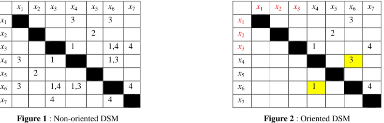
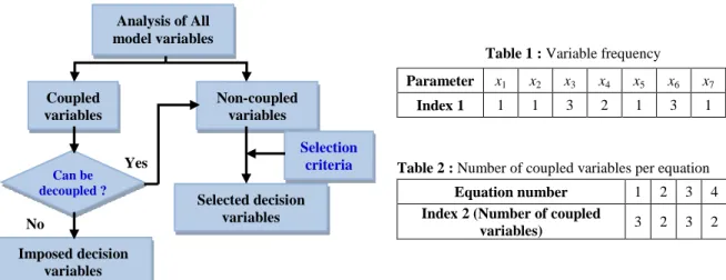
Figure
Documents relatifs
