Safe navigation within dynamic environments: a partial motion planning approach

HAL Id: pastel-00003661

https://pastel.archives-ouvertes.fr/pastel-00003661

Submitted on 18 Apr 2008

HAL is a multi-disciplinary open access archive for the deposit and dissemination of sci-entific research documents, whether they are pub-lished or not. The documents may come from teaching and research institutions in France or abroad, or from public or private research centers.

L’archive ouverte pluridisciplinaire HAL, est destinée au dépôt et à la diffusion de documents scientifiques de niveau recherche, publiés ou non, émanant des établissements d’enseignement et de recherche français ou étrangers, des laboratoires publics ou privés.

motion planning approach

Stéphane Renaud Petti

To cite this version:

Stéphane Renaud Petti. Safe navigation within dynamic environments: a partial motion planning approach. Automatic. École Nationale Supérieure des Mines de Paris, 2007. English. �NNT : 2007ENMP1516�. �pastel-00003661�

Collège doctoral

N° attribué par la bibliothèque

|__|__|__|__|__|__|__|__|__|__|

T H E S E

pour obtenir le grade de

Docteur de l’Ecole des Mines de Paris

Spécialité «Informatique temps réel – Robotique - Automatique»

présentée et soutenue publiquement

par

Stéphane Renaud PETTI

le 11 JUILLET 2007

SAFE NAVIGATION WITHIN DYNAMIC ENVIRONMENTS: A

PARTIAL MOTION PLANNING APPROACH

Directeur de thèse : Christian LAUGIER Co-Directeur de thèse : Thierry FRAICHARD

Jury

M. Claude LAURGEAU

Président

M. Luis MONTANO

Rapporteur

M. Thierry SIMEON

Rapporteur

M. Michel PARENT

Examinateur

Environments: A Partial Motion

Planning Approach

(Navigation sûre en environnement dynamique: une approche par

planification de mouvement partiel)

alors celles et ceux qui ont rendu cette aventure possible, pour prendre le temps de les remercier.

Au tout début, il y a une Société, Aisin AW, et certains de leurs membres qui ont cru et soutenu avec conviction mon projet. Je voudrais en particulier remercier mes collègues Européens M.Cervello, M.Knop, M.Diels et Japonais M.Kawa et, M.Fukaya. Puis il y a des rencontres capitales, avec l’INRIA tout d’abord, avec Michel Parent, qui a su immédiatement me faire confiance, Christian Laugier qui m’a accueilli sans hésitations dans son équipe et puis avec les Mines de Paris et Claude Laurgeau qui m’a ouvert les portes du centre de robotique CAOR, que je remercie sincèrement pour leurs marques de confiance et soutien sans failles.

Avec le travail qui avance de concert avec ses problèmes et doutes, ce sont les proches collègues de ces équipes qui permettent de reprendre confiance. Je remercie chaleureusement l’incontournable Chantal, reine d’IMARA et Armand, le Mc Gyver des Cycabs, pour leur humour, soutien et tous ces conseils avisés dont ils me faisaient part lors de nos pauses café matinales. J’ai à cœur de remercier également les talentueux Tony, Mickael, Laurent, Angele et mon vaillant collègue de bureau, l’extravagant mais non moins talentueux Rodrigo, pour toutes ces discussions passionnées sur des sujets aussi bien techniques que philosophiques, qui m’ont été si précieuses. Je voudrais également remercier Konaly et Fawzi pour la bonne humeur qu’il m’ont toujours communiquée aux Mines, merci également à Olivier, Arnaud, Yotam, et tous les autres membres d’IMARA, d’eMotion et du CAOR que je n’ai pas salué ici et pourtant qui m’ont permis grâce à chacune de nos conversations d’avancer un peu plus.

Bien entendu je n’oublie pas le plus vaillant de tous, Thierry Fraichard, qui armé de patience et conviction, m’a soutenu, conseillé et aidé tout au long de ce travail, durant plus de trois années, depuis le premier jour, jusqu’à ce dernier jour de soutenance et à qui je voudrais exprimer ma sincère gratitude.

Je voudrais également remercier Julien Akita, pour m’avoir offert la talentueuse illustration, unique, originale et pertinente qui préface ce manuscrit de thèse.

Et puis, par-dessus tout, à mes parents,

et leur foi en moi, indéfectible, qui m’a sans nulle doute portée jusque là, à ma femme, Ioulia,

sa gentillesse et sa patience, sans égale, et à mon fils, Alexandre

son énergie rafraîchissante et sa comprehension… et pour tout le reste, l’essentiel vraiment, qui ne trouve plus la place en ces quelques lignes.

Ainsi, je regarde aujourd’hui ces années de thèse, ces périodes de doutes, de stress mais aussi de satisfaction et voulais prendre le temps ici de rendre hommage à tous ceux qui ont fait que ces années ont été agréables et profitables et restent, plus qu’un souvenir, une expérience unique.

Safe Navigation Within Dynamic Environments: A Partial Motion Planning Approach 1 I Introduction 7 1 Introduction . . . 7 2 Problem . . . 8 3 Contributions . . . 9 4 Document Layout . . . 10

II Problem and existing works 15 1 The General Problem . . . 15

2 A Reactive Perspective . . . 16

3 A Deliberative Perspective . . . 24

4 Conclusion . . . 44

III The Approach 49 1 Introduction . . . 49

2 Theoretical Approach . . . 52

3 Discussion . . . 66

IV Case study of a Car-like System 71

1 Introduction . . . 71

2 Model of the Vehicle . . . 71

3 Model of the World . . . 76

4 ICS Computation . . . 76

5 Partial Motion Planning (PMP) Algorithm . . . 83

V Experimentations 97 1 Introduction . . . 97

2 The Cycab Platform . . . 97

3 Control Layer . . . 101

4 PMP Software Architecture . . . 106

5 Scenario 1 : Obstacle Avoidance . . . 108

6 Scenario 2 : Intelligent Crossing . . . 112

7 Scenario 3 : Autonomous Navigation . . . 116

8 Return of experience . . . 121

VI Conclusions and perspectives 123 1 Conclusion . . . 123

2 Perspectives . . . 125

VII Annexes 1 : Partial Motion Planning under Uncertainty 131 1 Partial Motion Planning and Uncertainty . . . 131

II.1 Obstacles that form local minima for the robot’s path. . . 16

II.2 Potential Field of an environment with two obstacles. . . 17

II.3 VFH* method. (source: [UB00]) . . . 18

II.4 Nearness Diagram method (ND). . . 19

II.5 Curvature Velocity method (CVM). . . 21

II.6 Dynamic Window approach (DWA). . . 21

II.7 Velocity Obstacle approach. . . 23

II.8 Exact vs. approximate representation. . . 27

II.9 Illustration of a random sampling based roadmap. . . 28

II.10 Denseness & Dispersion of a sampling. . . 28

II.11 Rapidly-exploring Random Tree principle. . . 30

II.12 Unicycle system. . . 31

II.13 Car-like system. . . 32

II.14 Representation of moving obstacles within CSxT. . . 36

II.15 Nonholonomic trajectory deformation (source [LB02]) . . . 40

II.16 Influence of the dynamics of a point mass robot on its safety. . . 42

II.17 Influence of the world’s dynamics on a system’s safety. . . 42

II.18 Influence of the time horizon on a system’s safety (τ -safety concept from [Fra01]). . . 43

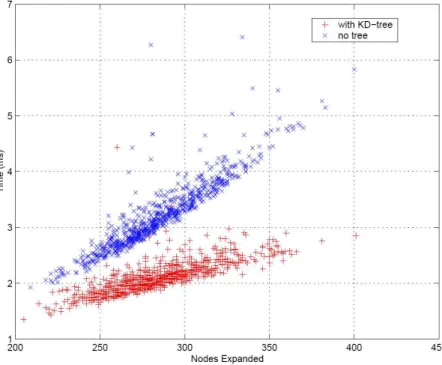
III.1 Running time versus number of nodes developed of two “Rapidly-Exploring Random Tree”-based randomized motion planners. (source: [BV02]) . . . 50

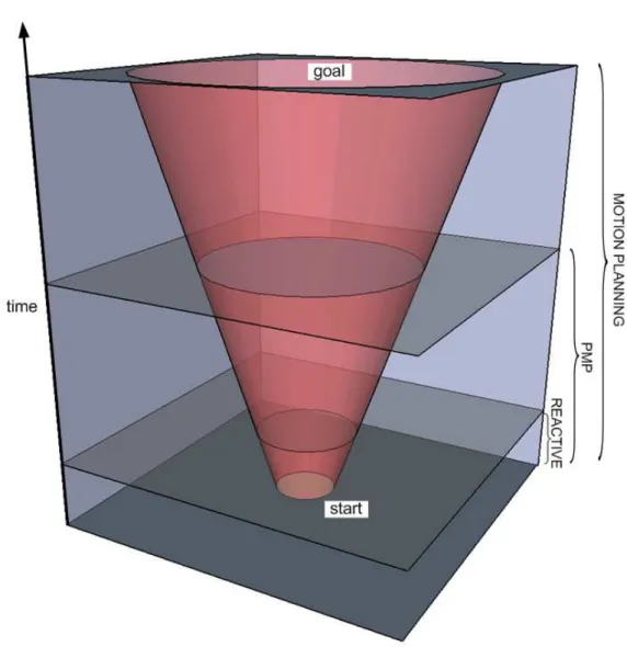
III.2 Partial Motion Planning vs. Reactive and Deliberative methods in ST . . 51

III.3 Partial Motion Planning in a known environment. . . 54

III.4 Prediction validity model. . . 55

III.5 Partial Motion Planning in a partially predictable environment. . . 56

III.6 Example of a tree of approaching trajectories of a spaceship to a satellite. (source: [PKB03]) . . . 57

III.7 Inevitable Collision Obstacle for a mass point robot system. (source: [LK01a]) 60 III.8 North-East East system and a static point obstacle. . . 61

III.9 North-East/East system and a static obstacle. . . 62

III.10North-East/East system and a moving point obstacle. . . 62

III.11North-East/East system and a moving obstacle of different velocities. . . 63

III.12Comparison between East, North-East/East and North-East/East/South-East systems and a static obstacle. . . 64

IV.1 Car-like system. . . 72

IV.2 Path shapes while turning at different vehicle speeds. . . 74

IV.3 bounding boxes used for geometric collision detection. . . 76

IV.4 Model of the environment. . . 77

IV.5 North-East system and a static point obstacle. . . 78

IV.6 Inevitable Collision Obstacle (ICO) of a static obstacle for a simple car. . 78

IV.7 ICO for a point obstacle P and a smooth car. . . 79

IV.8 Numerical calculation Inevitable Collision Obstacles (ICO) for a static and dynamic obstacle. . . 80

IV.9 Characterization of an Inevitable Collision Obstacle (ICO) at different ve-hicle speed. . . 81

IV.10Implicit ICO representation consists in finding inevitable collision states instead of the complete ICO characterization. . . 82

IV.11Inevitable Collision Obstacle (ICO) under arbitrary temporal approxima-tion for the East system. . . 83

IV.12Representation of the tree of reachable states for the car-like robot (100

nodes). . . 84

IV.13Inevitable Collision States within the PMP framework. Each state of the planned partial trajectory is verified to be an ICS with respect to the sur-rounding dynamic environment. . . 85

IV.14Notion of distance for non-holonomic systems. The double arrow represents the Euclidean distance whereas the nonholonomic distance is the length of the represented path composed of arc of circles and straight segments. . . 85

IV.15Influence of metric on trajectory generation. . . 86

IV.16Tree construction. . . 88

IV.17Examples of trajectories generated by the PMP. . . 89

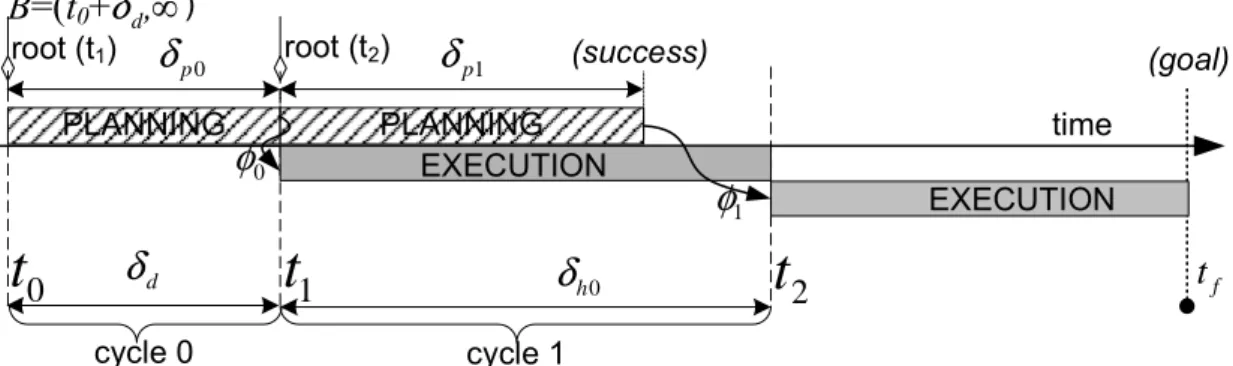
IV.18Sequence of PMP cycles in a general dynamic urban environment. . . 90

IV.19Sequence of PMP cycles in an environment highly cluttered with static and dynamic obstacles. . . 91

IV.20PMP generates large lookahead trajectories that can avoid U-shaped ob-stacles. . . 92

IV.21Trajectory lookahead with respect to the number of surrounding obstacles (data for 1 PMP cycle of 1 second). . . 92

IV.23Impact of steering speed constraint on trajectories generated during one PMP cycle of 2s, with a maximum steering angle of 0.5 radians. . . 92

IV.22Trajectory lookahead with respect to a cycle duration (data generated for an environment cluttered with 25 obstacles in each cases). . . 93

IV.24Impact of steering speed constraint on trajectories generated during one PMP cycle of 2s, with a maximum steering angle of 1.0 radians. . . 93

IV.25Impact of the choice of I on the generated trajectories. . . 94

V.1 The Cycab. . . 98

V.2 Several types of Cybercars. . . 98

V.3 Cycab hardware architecture. . . 99

V.4 Cycab high level architecture. . . 100

V.6 Execution of a reference trajectory in open loop. . . 102

V.7 Simulation of the tracking law (V.2) on Scilab software. . . 105

V.8 Error measurements of a trajectory tracking by the Cycab. . . 106

V.9 PMP software architecture. . . 107

V.10 PMP User Interface. . . 107

V.11 Simulation of pedestrians avoidance with PMP (partially known environ-ment). . . 109

V.12 Sensors used on the Cycab for perception and localization. . . 110

V.13 Obstacle object sensed by the Laser Scanner IBEO. . . 110

V.14 Cycab avoiding pedestrians. . . 111

V.15 Intelligent Crossing simulation. . . 113

V.16 Automated cars at an intersection. . . 114

V.17 Intelligent crossing experiment. . . 115

V.18 Simulation results of an autonomous navigation within a city. . . 117

V.19 Autonomous Navigation. . . 120

VI.1 PMP planning without uncertainty among moving obstacles. . . 125

VI.2 PMP planning with uncertainty among moving obstacles. . . 125

VI.3 Two autonomous Cycab’s using PMP and adapting to each other’s motion to collaboratively avoid collision . . . 126

VII.1Tree construction for planning under uncertainty. . . 133

VII.2In case motion uncertainty are not considered, the size of the cylinder bounding the car does not increase. In this case PMP plans a trajectory between the two static obstacles. . . 135

VII.3In case motion uncertainty is considered, the size of the cylinder bounding the car increases. In this case PMP plans a trajectory that bypasses the two static obstacles. . . 135

VII.4PMP planning without uncertainty among moving obstacles. . . 136

Introduction

1

Introduction

Driven by the dream of creating machines that would autonomously accomplish specific tasks, the interest to robotics goes back to early ages. From early automatons, to more recent robots1 _{[Cap20], these machines always inspired fascination. Nowadays, a robot}

is defined as a complex mechanical device equipped with sensors and actuators. It is designed to perform complex tasks autonomously or with human supervision, that are too dull, dirty, dangerous or accurate for humans.

A robot can perform several tasks, like mating or grasping parts, moving around to explore or survey. Regardless of the task, the robot performs a sequence of actions, eg moving an arm, closing grippers, or propelling itself. Then, each action will result in a motion. Thus, in order to successfully accomplish its task, a robot must be able to plan, ie find on its own and in advance, the sequence of motions to execute. In robotics, this specific problem of planning a motion a priori is addressed by motion planning and is at the heart of the work presented here.

In its general form, the motion planning problem consists in finding a priori, a sequence of motions that guides a system to a predefined objective. The calculation of a motion plan relies on models of both the system and the environment in which it is placed.

The basic motion planning problem is often referred to as path planning. The path planning problem consists in finding a collision free path, ie a continuous sequence of configurations. A configuration is the set of independent parameters representing the

po-1_{Term coming from the czeck robota, meaning drudgery.}

sition and the orientation of every part of the robot. Path planning, in its basic form, deals with free flying robots moving amidst stationary obstacles. The mechanical design of a free flying robot allows every part of it to freely rotate and translate such that its configuration changes are not constrained. In the late seventies, the concept of configu-ration space is introduced as a useful framework for the basic motion planning problem. In the configuration space, the robot is represented as a point and stationary obstacles as forbidden regions. The basic problem is therefore essentially geometric and deals with collision avoidance of stationary obstacles.

However, as soon as one of the main path planning hypotheses is broken, path calculation might not provide sufficient information for the robot to achieve its task. To begin with, the obstacles in the environment might move. In such a case, the time dimension must be considered. A time parametrization of the sequence of configuration becomes necessary. This introduces the notion of trajectory. In addition to the temporal aspects, the robot might be constrained by its kinematics or dynamics, which will limit its motion capability. Finally, the models on which motion planning relies might differ with the reality. The possible error, ie uncertainty impacts the motion at execution and might be incorporated at the planning level which further complicates the problem.

2

Problem

In robotics, it is important to always consider a robot as a real device with specific me-chanical architecture and constraints, intended to perform real tasks within a real world. Industrial robots used in manufacturing lines used to be the most common form of robots and motivated most of the work in path planning. Manipulators are built to ensure that the end effector can rotate or translate freely. They generally operate in a known fixed environment. Nowadays, other robots are emerging, such as servicing robots, that are also finding their way into entertainment, home, health care.

As for transportation, a large effort has been put in major industrial countries in the last decade, into developing new kinds of intelligent transportation systems, the Cybercars [Par97], as a mean to address the problems of congestion, pollution and safety raised by the increasing usage of personal cars. In the long term, these innovative transportation systems are envisioned to autonomously drive people within a city. The mechanical platform of these car-like robots, exhibit constraints (kinematic, dynamic and actuator constraints) that restrict their motion capabilities. Besides, they evolve in dynamic environments, cluttered with other cars or pedestrians. Cybercars are at the center of our research

interest. The main goal of this research work is to provide this vehicle, the capability to autonomously plan its trajectory to a predefined goal while avoiding obstacles. We consider the real urban context within which these vehicles are aimed to work.

Such an environment brings a major constraint that has not been mentioned until now. A system placed in the real world, cluttered with moving obstacles, has the obligation to plan a trajectory within a limited time, otherwise it might be in danger by the sole fact of being passive. This limited available time is a decision time constraint, imposed by the nature and dynamicity of the environment. This constraint must be strictly fulfilled at ex-ecution for the system’s safety and is therefore a hard real-time constraint. Although this constraint is of crucial importance, there is very little work in the literature taking this constraint into account explicitly. There are a few methods based on dynamic pro-gramming [PNIV01, Ste02] that succeed to plan very fast. The constraints of the system are however not easily incorporated, and the problems handled are usually of low dimen-sion. Latest probabilistic methods as well have shown efficient schemes [HKLR02, BV02] for simple systems. Nevertheless, no matter how fast these methods are, none of them provide a guarantee on the computation time upper bound and therefore none of them account for the real-time constraint explicitly.

Therefore our problem turns into trajectory planning for a system : 1. under kinematic and dynamic constraints of the system

2. evolving within a dynamic environment 3. under a real time constraint

3

Contributions

• In our work we address the problem of navigation within a dynamic environment from a motion planning perspective. The main contribution of this work is to ex-plicitly consider the real-time constraint dictated by a dynamic environment. Now, given the intrinsic complexity of the motion planning problem, computing a complete motion to the goal within the time available is impossible to achieve in most real situations. Partial Motion Planning (PMP) is the answer to this problem proposed in this work. PMP is a motion planning scheme with an anytime flavor: when the time available is over, PMP returns the best partial motion to the goal computed so far.

• Safety becomes a major issue for partial planning. When collision free condition might suffice for path planning problems, this is not the case when dealing with

dynamic environments. Safety must be considered from a different perspective and other criteria must be considered. At first the dynamics of the system must be taken into account. Indeed a dynamic system has a drift caused by its inertia, that moves a system even when commands are applied. Furthermore, when dealing with a dynamic environment, it is fundamental to account explicitly for the motion of the obstacles. Otherwise, even though the last state might be collision free, it might still be in danger. A guarantee that the system will never end up in a critical situation yielding an inevitable collision must be given. The second contribution of our work addresses this aspect and studies the safety issue from a more complete perspective suitable for our problem. The answer proposed in this work to this safety issue relies upon the concept of Inevitable Collision States (ICS) [FA04]. ICS is a concept that encompasses the dynamics of both the system and the moving obstacles. A strong safety guarantee is given to a partial plan by computing ICS-free partial motions. • Finally, the last contribution of this work is to demonstrate the efficiency and

ro-bustness of the approach and integrate the algorithm on a real platform, a Cycab. We present the integration of PMP within a real navigation architecture. This archi-tecture mainly rely on a laser scanner for the model perception and construction and a Real Time Kinematics GPS for the localization. As for the model prediction, we assume it is provided to our planner. We believe this assumption realistic consider-ing latest results on model’s prediction [WTT03, VF04], however we do not address it in this work. Nevertheless, we present the advantage of coupling PMP with such an approach, a Simultaneous Localization, Mapping and Moving Objects Tracking (SLAMMOT) algorithm. Furthermore, we detail how the planning and execution interleave. The execution of the trajectory is handled by a low level controller, a tra-jectory tracking controller, aimed at properly execute the planned tratra-jectory. Actual experiments on a real platform, the Cycab are presented to validate the approach and the overall architecture.

4

Document Layout

We complement in chapter §2 the description of the problem and present a state of the art of the related work. Our approach is then presented in chapter §3. In chapter §4 we present an adaptation of PMP to the case study of a car-like robot and we present the results of our simulations as well as our experimentation on a real platform, that we have carried out for this case study in chapter §5. Finally, in chapter §6 we draw our final conclusions on the approach and, from the return of experience of our experiments, we discuss the perspective of this work.

Introduction

Le rêve de créer des machines qui pourraient accomplir des tâches spécifiques de manière autonome, et l’intérêt porté à la robotique plus généralement remonte à très longtemps. Des premiers automates aux plus récents robots, ces machines ont toujours engendré de la fascination. De nos jours, un robot est défini comme un dispositif mécanique com-plexe équipé de capteurs et d’actuateurs. Ils sont conçus pour accomplir, soit de manière autonome, soit sous la supervision d’êtres humains, des tâches complexes qui sont trop ennuyeuses, sales, dangereuses ou trop précises pour l’homme.

Un robot peut effectuer de nombreuses tâches comme l’assemblage et la saisie d’objets, ou l’exploration. Indépendamment de la tâche, le robot doit effectuer une séquence d’actions, eg. bouger un bras, fermer des pinces ou se propulser. Puis, chaque action conduit à un mouvement. Ainsi, afin d’accomplir avec succès une tâche, un robot doit être capable de planifier, cad. trouver par lui même et à l’avance, la séquence d’action à exécuter. En robotique, le domaine qui aborde ce problème de déterminer à priori un mouvement, s’appelle la planification de mouvement et se trouve au coeur du travail présenté ici.

Dans sa forme générale, le problème de planification de mouvement consiste à trouver a priori une séquence de mouvements qui amènent un système à un objectif prédéfini. Le calcul de ce plan s’appuie sur un modèle du système et de l’environnement dans lequel il évolue.

Dans sa forme de base, le problème de planification de mouvements est appelé planifica-tion de chemin. Le problème de planificaplanifica-tion de chemin consiste à trouver un chemin sans collision, cad. une séquence continue de configurations sans collision. Une configuration est un ensemble de paramètres indépendants qui représentent la position et l’orientation de chaque partie d’un robot. Dans sa forme primitive, le problème de planification de chemin considère des objets qui évoluent sans contraintes dans un environnement sta-tique. Le concept mécanique d’un robot "free flying" permet à chacune des parties de ce robot d’effectuer rotation et translation librement, de telle sorte que chaque changement de configuration ait lieu sans contraintes. Dans la fin des années ’70, le concept d’espace des configurations est introduit comme un formalisme très utile pour le problème de la planification de chemin. Dans l’espace des configurations, le robot est représenté par un point et les obstacles comme des régions de l’espace interdites. Le problème de base est alors essentiellement géométrique et porte sur les évitements d’obstacles statiques.

Cependant, des que une des hypothèses de base du problème n’est plus remplie, il est probable que le calcul de chemin ne fournisse plus alors toutes les informations nécessaires au robot pour accomplir sa tâche. Tout d’abord, les obstacles dans l’environnement peuvent

bouger. Dans ce cas, l’aspect temporel doit être pris en compte. Une parametrisation en fonction du temps de la séquence de configuration devient alors nécessaire. Cela introduit la notion de trajectoire. En plus des aspects temporels, le robot peut être contraint par sa propre cinématique ou dynamique, ce qui limite ses mouvements. Enfin, le modèle sur lequel la planification de mouvement se base, peut être différent de la réalité. Cette erreur possible, ou incertitude a un impact sur le mouvement lors de son exécution et peut être prise en compte dés la planification ce qui complique largement le problème.

Problème

En robotique, il est important de toujours considérer le robot comme un dispositif réel avec une architecture et des contraintes mécaniques spécifiques, dans le but d’accomplir des tâches réelles dans un monde réel. Les robots industriels utilisés dans les usines réelles étaient jusqu’à présent les plus communs et ont motivé l’essentiel du travail en planification de chemin. Les bras manipulateurs sont conçus pour permettre à son extrémité de tourner ou translater librement. Ils opèrent en règle générale dans un environnement fixe et connu. De nos jours, de nouveaux types de robots émergent, comme des robots grands publics que nous trouvons dans le divertissement, à la maison ou les soins de santé.

Quant au transport, un effort important, dans la majeure partie des pays industrialisés durant les dix dernières années, a été fait pour développer de nouveaux types de systèmes de transports intelligents, les Cybercars, comme moyen pour affronter les problèmes de congestion, pollutions et sûreté, soulevés par l’usage toujours grandissant des véhicules personnels. A long terme, il est envisagé que ces nouveaux systèmes de transports intel-ligents, soient capables de transporter les gens au sein de la ville, de manière totalement autonome. Ces robots voitures sont soumis à des contraintes (mécaniques, dynamiques, au niveau des actuateurs) qui restreignent la capacité de mouvement du système. De plus, ils évoluent dans un environnement dynamique, ou d’autres objets (voitures ou piétons) évoluent. Les Cybercars sont au centre de notre travail de recherche. L’objectif essen-tiel de ce travail est de pouvoir fournir à ce type de véhicule, la capacité de planifier de manière autonome sa trajectoire vers un but choisi tout en évitant les différents obstacles. Nous considérons l’environnement urbain réel, comme étant celui où ces véhicules doivent pouvoir progresser.

Ce type d’environnement apporte une nouvelle contrainte, dont nous n’avons pas en-core parlé. Un système placé dans un environnement réel, peuplé d’obstacles mobiles, a l’obligation de planifier une trajectoire dans un temps limité, sinon il peut se retrouver en danger, par le seul fait d’être passif. Cette limite de temps disponible est une contrainte

de décision imposée par la nature et dynamicité de l’environnement. Cette contrainte doit être remplie strictement durant l’exécution du mouvement et est pour cette raison une contrainte temps réel dure. Bien que cette contrainte soit d’importance cruciale, il y a paradoxalement peu de travaux dans la littérature qui prennent cette contrainte en compte. Il y a certaines méthodes basées sur la programmation dynamique qui réussissent à plan-ifier très rapidement. Les contraintes liées au système sont cependant difficiles à prendre en compte et les problèmes abordés sont généralement de dimension peu élevée. Les ré-centes méthodes probabilistes ont également montré qu’elles peuvent être très efficaces pour des systèmes simples. Néanmoins, aussi rapides soient elles, aucune de ces méthodes ne garantit une borne en temps de calcul et ainsi aucune ne prend en compte de manière explicite cette contrainte temps réel.

Ainsi notre problème devient un problème de planification de trajectoire pour un système qui :

1. est soumis à des contraintes cinématiques et dynamiques 2. évolue dans un environnement dynamique

3. est soumis à une contrainte temps réel

Contributions

• Dans ce travail, nous adressons le problème de navigation en milieu dynamique d’un point de vue planification de mouvement. La contribution principale de ce inclu-travail est la prise en compte explicite de cette contrainte temps réel définie par l’environnement. Compte tenu de la complexité intrinsèque au problème de planifi-cation de mouvement, calculer un plan vers le but dans un temps limité est impossible dans la plupart des cas. La planification de mouvement partiel (PMP) est la réponse apportée à ce problème que nous proposons dans ce travail. PMP est une méthode de planification de mouvement ayant la faculté de retourner à tout moment le meilleur plan possible vers le but qui a été calculé jusqu’ici.

• La sûreté devient un élément essentiel pour la planification partielle. Quand la con-dition de non collision est suffisante pour les problèmes de planification de chemin, ce n’est plus le cas lorsqu’un environnement dynamique est pris en compte. Dans ce cas la notion de sûreté doit être étudiée sous une autre perspective avec d’autres critères. Tout d’abord, la dynamique du système doit être prise en compte. Par exemple, l’inertie d’un système dynamique peut le faire dériver sans qu’aucune com-mande ne soit appliquée sur celui-ci. De plus, quand un système évolue dans un

environnement dynamique, il est fondamental de prendre en compte de manière ex-plicite le mouvement des obstacles. En effet, quand bien même un état est sans collision à un moment donné, il se peut qu’il soit en danger à l’étape suivante. Une garantie sur le fait qu’un système ne va jamais se mettre dans une situation critique qui aboutirait à une collision inévitable, doit être fournie. La seconde contribution de ce travail traîte cet aspect et étudie la sûreté sous un angle plus complet et approprié à notre problème. La réponse proposée dans ce travail concernant le problème de sûreté réside dans l’utilisation du concept des Etats de Collisions Inévitables (ICS). ICS est un concept qui inclut la dynamique du système et de l’environnement. Une garantie de sûreté forte est donnée à un plan partiel en calculant un plan sans ICS. • Enfin la dernière contribution de ce travail consiste à démontrer l’efficacité et ro-bustesse de l’approche et d’intégrer l’algorithme sur une plate forme réelle, un Cy-cab. Nous présentons l’intégration de PMP au sein d’une architecture de navigation réelle. Le couplage avec la perception est essentiellement basé sur l’utilisation d’un laser scanner et d’un GPS cinématique temps réel (RTK). L’avantage de l’intégration avec un algorithme de localisation et construction de carte simultanée (SLAM) est également présenté. Quant à la prédiction du modèle, nous partons du principe que cette information est fournie au planificateur. Nous pensons que cette hypothèse est réaliste compte tenu des récents travaux en la matière, cependant nous n’abordons pas ce sujet dans ce travail. De plus nous détaillons comment la planification et l’exécution se synchronisent. Le contrôleur bas niveau est un algorithme de suivi de trajectoire qui a pour but d’exécuter la trajectoire planifiée de référence. Des ré-sultats d’expérience sur plateforme réelle sont présentés pour valider l’approche et l’architecture générale.

Plan du document

La description plus détaillée du problème ainsi que de l’état de l’art sont présentés dans le chapitre §2. Notre approche est ensuite présentée dans le chapitre §3. Dans le chapitre §4 nous présentons l’adaptation de notre approche à un cas particulier, celui du robot type voiture et présentons dans le chapitre §5 les résultats de simulations et expérimentaux sur plateforme réelle, que nous avons pus faire pour ce cas d’étude. Finalement, dans le chapitre §6 nous présentons nos conclusions finales et discutons des perspectives possibles de ce travail compte tenu du retour d’expérience des tests entrepris.

Problem and existing works

1

The General Problem

From a general point of view, this work is aimed at developing a navigation method for autonomous vehicles evolving within dynamic environments. A navigation method consists in generating and executing a motion to a predefined objective while avoiding the obstacles present in the environment. Such methods are at the heart of the motion strategy of autonomous robots. In the literature, the general navigation problem has been essentially addressed from two distinct perspectives, the reactive one and the deliberative one.

The reactive approaches compute one action at a time to be performed during the next time step. The deliberative approaches, at the opposite, are aimed at calculating the completesequence of actions to reach the goal.

In the following section, we propose to review the most significant reactive approaches and discuss their disadvantages. Following this presentation we concentrate on the de-liberative approaches, namely motion planning. We review the different methods and their capability to handle different constraints. We finally discuss recent techniques that have motivated us to formulate the problem addressed in this work from the deliberative perspective.

2

A Reactive Perspective

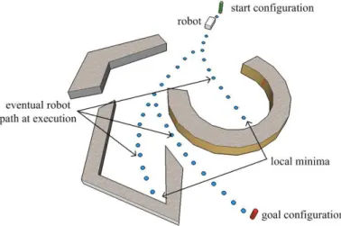
Initial work on real robots required the ability to “react” to the environment in order to avoid obstacles. The necessity to build schemes fast enough such that the robot does not collide with its environment led several authors to propose algorithms later referred to as reactive approaches [BK91, Kha96, FS98, KS98]. In order to be fast and therefore limit the computation time, a reactive scheme consists in calculating at each time step only the next action that will move the robot closer to the goal without colliding with its surroundings. The complete knowledge of the environment is not necessary to compute a single motion, and in most cases the local information of the direct surrounding of the robot will be sufficient. Thus, reactive methods are very well suited for the navigation of real robots equipped with on-board sensors (ultrasonic, laser, ...). This navigation refers also to as sensor based navigation. However, the calculation of one single motion step limits the lookahead ie the ability to anticipate and judge whether a better path would be available. As a consequence, robots can be navigated to areas from which it will never escape. In fig. II.1 the robot might be trapped at execution in two obstacles. These ¨traps¨ or local minima can be formed by obstacles of concave shape and cannot be anticipated using reactive schemes. This certainly is their major disadvantage.

Figure II.1: Obstacles that form local minima for the robot’s path.

Another consequence stemming from the lack of lookahead is the problem these schemes exhibit in some situations to converge to the goal rapidly. Nevertheless, several reac-tive methods paved the road to recent complex and efficient techniques. We propose to discuss these methods, that mostly differ from the assumptions on the characteristics of environment and the robot itself.

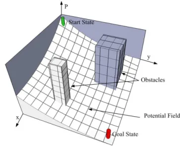
by combining the attractive force of the goal and repulsive forces of the obstacles. It is very well suited for small mobile robotic platforms equipped with ultrasonic sensors for instance. A potential field (represented as a mesh in fig. II.2 of value P) is calculated online from the obstacle information given by the sensors and the next action is calculated. Interestingly, in case a complete model of the environment is provided, a complete potential field of the world can be computed. In this case a global form is derived using a navigation function which is also referred to as a feedback motion planning scheme [RK88]. However, the calculation of such a function, without other local minima than the goal, is extremely difficult in general, and has been developed for circular obstacles mainly. Another disadvantage of this method is that it is not suitable for dynamic environment as the force calculation does not account explicitly for the obstacles motion.

Figure II.2: Potential Field of an environment with two obstacles.

• The Vector Field Histogram (VFH) method introduced in [BK91] uses a 2D Cartesian histogram as a world model. It can be updated in real time using in-formation from on board sensors. This histogram grid is based on earlier certainty grid [Mor88] and occupancy grid [Elf89] where each cell information represents the probability of having an obstacle at this point. This grid is translated into a po-lar histogram and the possible decision results from using the grid below a certain threshold value. A cost function based on the goal direction, the robot’s current orientation and the wheels angle, is used to make the decision between the potential authorized directions and define the orientation of the next step motion. The speed is calculated at a second stage, as a function of the distance from the mobile robot and the goal state. This approach is limited by the use of arbitrary heuristics the

tuning of which largely influence the behavior of the algorithm. Besides, the use of polar grids reduce the field of view and thus prevent sometimes the system from choosing the most suitable orientation. An extension, VFH* method, is proposed later in [UB00] to improve the local nature inherent to the original scheme. The idea consists in using a map and calculate a small tree in CS , of a sequence of collision free pose, ie position and orientation of the system, a few steps ahead and from dif-ferent starting configuration (see fig. II.3). This sequence is therefore geometric and cannot be used directly as a control input for the robot. The local search is based on a graph search using dynamic forward programming. This augmented lookahead improves indeed the faculty of the robot to escape local minima, while providing a smarter indication on the next orientation to use, thus improving the convergence of the scheme. This method however does not consider dynamic environments. Even though, kinematic constraints are considered in a variant of this scheme [UB98], this method does not account for dynamic constraints (from the system and the environment) which is its major limitation.

(a) exploration tree and executed trajectory (1 step ahead)

(b) exploration tree and executed trajectory (2 steps ahead)

(c) exploration tree and executed trajectory (5 steps ahead)

Figure II.3: VFH* method. (source: [UB00])

• The Nearness Diagram (ND) [MM00] method consists in analyzing a situation from two polar diagrams. These diagrams are built by means of on board sensors. One diagram is used to extract information of environmental characteristics and identify the immediate goal valley (see fig. II.4(a)), and the second one is used to define the safety level between the robot and the obstacles by identifying the closest one (see fig. II.4(b)). ND is similar to the VFH method that uses polar histogram. The kinematic constraints of mobile robots are taken into account in [MMSV02] similarly to all other previously presented methods, by approximating its path by straight segments and arc of circles. The decision is taken by a choice of suitable

controls in the ego-kinematic space, which is a representation of the world in terms of distance and radius of curvature that describe the arc of circle from the robot to an obstacle. The Global ND [MMSA01] then is a hybridization of ND combined with a NF1 function in order to get more lookahead and avoid traps similarly to other methods. An ego dynamic space is presented to account for dynamic constraints in [MMK02].

(a) First step calculation based on free sectors. (b) Second step calculation for safety check

Figure II.4: Nearness Diagram method (ND).

• The Curvature Velocity method (CVM) was introduced in [Sim96] as a local ob-stacle avoidance technique for indoor mobile robots accounting for their kinematic and dynamic constraints (acceleration and velocity bounds). This technique con-sists in finding the next suitable speed (rotational w and linear v speed) as this information is directly a command for the mobile robot. Given the physical and environmental constraints on the velocities, commands for the robot are chosen by optimizing an objective function. The objective function is designed so as to prefer high speeds, curvatures that travel longer before hitting obstacles and should try to orient the robot to head in the desired goal direction. The main principle consists in directly exploring the velocity space VS, the space of all possible speed for the robot. The main difficulty consists in defining obstacles of the real environment in this VS. The CVM method uses arc of circles of different curvatures (noted ci’s) in order to consider the robot’s kinematics. Distances to the obstacle (noted di’s) that the robot would travel before hitting the obstacle, are calculated for all curvatures (in fig. II.5(a), obstacles are represented by circles and the distance between the robot, located at the origin, and the obstacles, by the distance of the arc of circles

hiting the obstacles). Then, the method consists in mapping this distance and cur-vature information from the workspace W to the velocity space VS. Interestingly, in VS, the curvature information is described by a half-line. This half-line defines the boundary of a region of a specific weight, which is the shortest distance to an obstacle as illustrated in fig. II.5(b). In order to account for the physical limitation of the system, a maximum acceleration constraint is set, and a maximum velocity defined in VS. In fact, at each step, a new velocity bound is calculated from the sys-tem’s acceleration bounds and the time step (see fig. II.5(c)). Finally, the candidate velocity pair that maximizes the objective function is chosen as the best candidate for the next step. The disadvantage of the weighted cost function is to depend on the choice of weights which might result in a non uniform robot’s behavior, depending on the situation. The Steering Angle Method [FBL94] is very similar to this method but only rotational velocity is calculated. The Lane-Curvature method is presented later in [KS98], to overcome the main shortcomings of the CVM. For instance, at an intersection, CVM method fails to guide the robot into an open corridor toward the goal direction. In fact it often passes over some paths which are at right angles to the current robot’s orientation. Besides, as all local methods, it lets the robot head towards an obstacle, even if there is a clear space around it. These problems stem from the fact that CVM chooses commands based on the collision-free length of the arcs assumed to be robot’s trajectories and it does not pay much attention to collision free directions. It seems that the Lane Method is here to finally pre-process the environment without considering the robots dynamic. Therefore LCM turns into a two step approach that takes the free directions into account in a first step and then the collision free arc length. In order to find a heading direction the lane method divides the environments into lanes oriented in the direction of the desired goal heading. This methods account for more constraints as VFH, however, the dynamic environment is not handled more explicitly.

• The Dynamic Window Approach (DWA) introduced in [FBT97] is certainly one of the most popular reactive approach. The DWA is in many ways similar to the CVM method, with the difference that a discretized velocity space is built. A dynamic window of feasible velocities is built around the robot’s velocity. A velocity is considered solution if it fulfills the systems constraints of maximum speed and maximum acceleration. Furthermore, the velocity must allow the robot to stop before hitting the obstacle. In case nonholonomic systems are considered, arc of circles are considered instead of straight lines. To overcome the lack of lookahead, an augmented method, the Global DWA, is presented by [BK99]. In addition to the sensor readings used to built the model, a map is incorporated in order to allow

(a) Representaiton of circular obstacles in W and the distance of the robot to the obstacles.

(b) Representation of regions n CS of different weights accounting for the proximity of an obstacle to the robot.

(c) Repesentation in CS of the velocity constraint and physical limitations.

Figure II.5: Curvature Velocity method (CVM).

better lookahead. Thus, the DWA is combined with a grid based global navigation function in order to get a more goal directed scheme and get information about the free space connectivity in order not to be trapped in local minima. This method is limited by the model construction as well as the parameters tuning. This method finally is mostly suitable for static or low dynamic environments.

(a) dynamic window for a holonomic system (b) dynamic window for a nonholonomic system

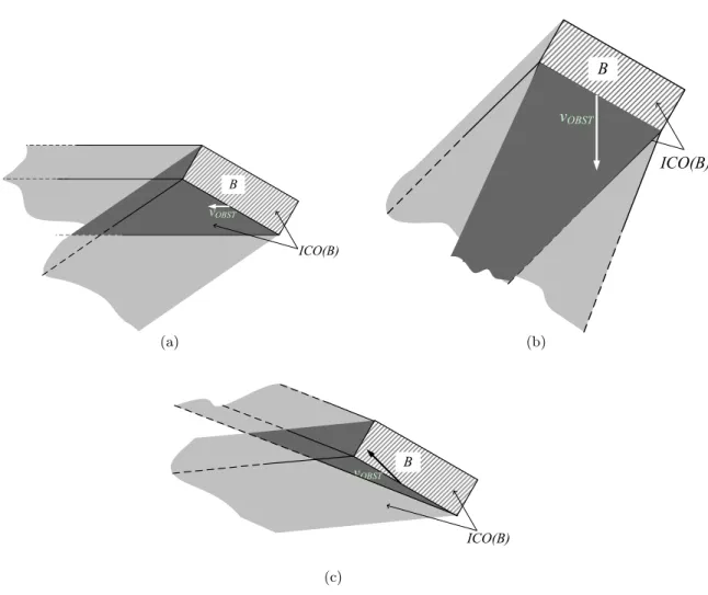
• The concept of Velocity Obstacles (V O) introduced in [FS98], allows the repre-sentation within the velocity space of moving obstacles (see fig. II.7(a)). This tech-nique differs from the previous one by the capability of taking explicitly into account the environment dynamicity. Velocities (ie speed and direction) of the surrounding objects are assumed to be known. Having this information, moving obstacles are transposed into the velocity space (the velocity pair vxand vy, resp. along the x-axis

and y-axis in this case) and represented by velocity obstacles, regions of forbidden velocities. A velocity if forbidden if it eventually yields a collision with the moving object. Velocity for the next time step is selected among the subset of allowed ve-locity vectors. This method also permits to consider objects moving along arbitrary trajectories (see fig. II.7(b)). An incremental motion planning strategy is used in [LSSL02] using this concept. The incremental approach calculates at each time step, a collision free velocity vector. A sequence of such admissible velocities is chosen and supplied to the system. From the resulting position another free velocity vector is calculated according to the model of the environment, one step further. A tree of free velocity controls is built defining thus a complete plan. This technique is the first approach to our knowledge that is aimed at calculating a few motions in ad-vance. In order to account for dynamic and kinematic constraints, a pre-calculation of admissible velocities Vadm has to be done. Each node is determined by applying

a safe linear constant velocity. For real world applications however, the errors in-troduced during the transition between two different linear velocity control, might put the robot in danger as the real robot displacement will differ from the piecewise linear one which is assumed when calculating safe controls.

• A more recent approach [OM05] presents a method that addresses robot subject to kinematic and dynamic constraints evolving within a dynamic environment. Simi-larly to several methods already described, the key of this method consists in map-ping these constraints into a velocity-time space VSxT. Unlike DWA, the proposed

method accounts for the motion of the surrounding obstacles. The possible paths are represented using a similar path discretization as in CVM or DWA (arc of circles and straight segments). Then, for every surrounding moving obstacle a surface of forbidden velocities is calculated based on possible collisions. Limiting the window of feasible velocities to account for the dynamics of the system, the best velocity is chosen within the free velocity space while maximizing the convergence to the goal. Interestingly, this method enhances the concept of the DWA approach by considering dynamic environments.

Thus, reactive approaches have been very popular and widely used on several real plat-forms, thanks to their ease of implementation, a low computation cost and the actual

(a) construcion of a velocity obstacle (b) representation of nonlinear velocity obstacles

Figure II.7: Velocity Obstacle approach.

difficulty to observe and model the environment. However, their inherent limitation is poor lookahead that conducts the robot to be trapped in local minima during its trip, and as a consequence a weak convergence to the goal. Besides, reactive methods are very efficient when they directly work in the velocity space that is in most cases the natural command space of the robot (steering angle control homogeneous to the rotational speed w and longitudinal speed v). However, certain systems exhibit constraints that are diffi-cult to model explicitly in this VS. Car-like robot for instance have kinematic constraints that are taken into account by considering its path as a sequence of arc of circles and straight segments [Sim96]. This approximation however introduces a discontinuity in the path curvature, which represents an instantaneous change in the wheels’ orientation. At execution, the system has to stop at each curvature discontinuity, ie at each junction be-tween a straight segment and an arc of circle, otherwise the real motion cannot comply with the one calculated by the reactive scheme. Dynamic constraints as well must be approximated to be taken into account. It is done by reducing the control space to a set of physically possible controls in order to account for the bounded acceleration and deceleration of a system [FBT95, Sim96, MMSV02]. As we have described, even though most of the reactive methods have been recently modified so as to improve these limita-tions, the most important issue remains the fact that, at the exception of [FS98, LSSL02] and [OM05], none of the presented schemes do account explicitly for the dynamic nature of the environment, hence becoming useless in such an environment. Therefore, in our opinion, reactive methods present significant weaknesses in the context of our work. This

observation is the ground motivation for us to address our problem from the deliberative perspective.

3

A Deliberative Perspective

3.1 The Basic Problem

The paradigm of deliberative approaches is usually referred to as motion planning. We define the motion planning problem as:

Definition 1

Motion planning is a priori determination of the motion strategy based on a model of the world that will take the robot from its current position to a goal position.

The basic motion planning problem has been essentially motivated by the industrial use of manipulator arms robots ever since 1961 with the introduction of Unimate 1_{. Indeed,}

widely used in production lines, these robots operate via an end effector which is mechan-ically designed to freely translate and rotate in usually a known and fixed environment. Under these two conditions (a robot free of move and a static environment), the basic mo-tion planning problem consists in defining a sequence of pose or configuramo-tion of a robot, collision free to the goal. Formally, a configuration is the set of independent parameters that uniquely define position and orientation of every part of a robot, and the configu-ration space CS, the set of all possible configuconfigu-rations [LP81]. Such a sequence is usually referred to as a path and the basic problem as path planning.

The context is particularly important in robotics. As soon as one goes beyond the scope of manipulator arms, the main hypotheses of path planning are violated. This is the case in our work since it focusses on intelligent cars evolving within cities. Indeed, cars are robots constrained by their kinematics and dynamics. Besides, in our work they are assumed to evolve in an environment cluttered with moving obstacles (pedestrians, other cars). This latter constraint, the dynamic nature of the urban environment, particularly complicates the motion planning problem as we will see in this chapter.

In the following of this chapter, we first present in section 3.2 the main types of motion planning strategies and their motivation from a complexity point of view. We explain the basics of these techniques, as this will be necessary latter in this work. At second, detail the extensions of the basic problem that we just mentioned, as we believe this will

1_{In 1961 the first Unimate robot, manufactured by Unimation Inc., is shipped from Danbury,}

Con-necticut and installed in a plant of General Motors in Trenton, New Jersey. The robot lifts pieces of metal from die casting machine and stacks them.

ease the understanding of the remaining of this work. Thus, in section 3.3.1 we detail the constraints that impact the original motion planning problem, namely the kinematics and the dynamics. Then, in section 3.4, we introduce formally the main concern of this work,ie the problem of motion planning in a dynamic environment and present the related existing works. Finally, we conclude this chapter by pointing out fundamental observations in section 3.5 and 3.6 that lie at the heart of this work.

3.2 Complexity and Main Strategies

In this section, we review the main motion planning strategies that have been developed over the last years. We study the evolution of these basic methods, from the perspective of algorithm’s completeness and detail the three major classes of motion planning strategies, namely the complete approaches, the resolution complete approaches and the probabilistic complete approaches.

Complete Algorithms Approaches Motion planning algorithms are evaluated in terms of their completeness, which is defined as follows:

Definition 2

An algorithm is said to be complete if it returns a valid solution to the motion planning problem if one exists or returns failure if there is no solution.

We do not review in this work the well-known complete motion planning approaches addressing the basic motion planning problem. For a thorough study and state of the art of these methods, we refer to the work of [Lat91]. Even though, the study of the extension of the basic motion planning problem will be presented in the next section, let focus just a moment on complete schemes that address such extensions to make the following observation: there exist very little work, and to our knowledge only the work of [O’D87] and [FS89], which propose complete motion planning approaches, for extensions of the basic problem in very simple cases. In [O’D87] a body moving from a state A to a state B is considered, while avoiding collision with a set of moving obstacles. The motion must satisfy an inertial constraint: the acceleration cannot exceed a given bound. In this work a polynomial-time motion-planning algorithms is given for the case of a particle moving in one dimension. In [FS89] a path planning technique in the presence of moving obstacles is presented, based on the exact cell decomposition technique. The methodology is to include time as one of the dimensions of the model of the world. This enables the authors to regard the moving obstacles as being stationary in this extended world. For a solution to be feasible, the robot must not collide with any other moving obstacle, and

also must navigate without exceeding the predetermined range of velocity, acceleration and centrifugal force. The authors investigate an appropriate model to represent the extended world for the path-planning task and give a time-optimal solution using this model.

An explanation for such a few available techniques comes from the study of the complex-ity of the complete motion planning algorithms. It is interesting indeed to have a better understanding on the difficulty of the problem. Both lower bounds which give indication on the difficulty of the problem itself, and upper bounds given by the existence of algorithms, have been presented in the literature. In 1979, the first lower bound complexity of motion planning is proved to be PSPACE-hard [Rei79]. Several following results for a variety of extensions also showed PSPACE complexity (Planar linkage [HJW84], multiple rectangles [HW86], planar arm [JP85]). The decidability of the motion planning problem, which re-lates to the fact that a solution to the problem exists, was established by [SS83] using the cylindrical algebraic decomposition in the 3D workspace. This algorithm set the first up-per bound for the global motion planning problem and gives a time complexity to be twice exponential in the dimension of the space, and polynomial in the geometric complexity of the obstacle. A few years later, a roadmap based algorithm solved the same problem with singly exponential complexity in the space dimension [Can87]. This algorithm remains the most efficient algorithm currently available for solving the general motion planning prob-lem. Good solutions exist, however for limited cases only, eg polynomial-time algorithms when the workspace is a plane [OY82, LS85, ABF88]. As soon as further constraints are added, the problem becomes intractable (eg kinematic constraints NP-hard [RW98], dynamic constraints NP-hard [RS85], [CR87]). As a consequence, the discouraging com-plexity of the problem and the need for practical algorithms motivated some authors to weaken its requirements.

Resolution Complete Approaches The main idea is to discretize the search space and build a conservative approximation of the free space. Some approaches conduct a search over grids of fixed resolution in the explored space. The size of the grid defines the resolution of the algorithm. They result in weaker guarantees that the problem will be solved. Indeed, for a given resolution, if a solution exists, the algorithm will find it, if no solution is found, it does not mean the problem does not have a solution, since the solution might have been found for a smaller resolution level. These approaches are called resolution complete. In [DXCR93] the first polynomial-time algorithm with a proved goodness and running time bound is presented, for a robot moving from a starting position to a goal position while obeying both kinematic (joint limitations and obstacles) and dynamic (velocity and acceleration) constraints. These planning techniques enable near optimal solution for practical problems to be found [SD88, SH85, JC89]. Using this

approach, the work of [Fra99] presents a near time optimal approach that searches the solution trajectory over a restricted set of "canonical trajectories" accounting for both dynamic of the system and the environment.

Probabilistically Complete Approaches The first randomized approaches appeared in the mid of 90’s, in order to improve existing methods [BLL92]. In the randomized potential field approach, a heuristic function is defined on CS that attempts to steer the robot toward the goal through gradient search. If the search becomes trapped in local minimum, random walks are used to help escape. The first planning technique completely based on random sampling is the Probabilistic Roadmap Planner (PRM) [KSLO96, OS96], now recognized as a major popular and efficient technique.

Figure II.8: Exact vs. approximate representation.

The main idea for PRMs is to avoid the explicit construction of the free space. It is approximated by random sampling instead. This approach consists in probing the space with a random sampling scheme and a detection collision module. Fig. II.8 illustrates an explicit representation of the free space on the left, where each obstacle is completely defined as opposed to an approximated one on the right where states are individually tested and considered as part of an obstacle, or part of the free space. Nearby configurations are connected by computing a path using a local planner so as to construct a roadmap ie a graph within CS (see fig. II.9). The roadmap is later used to solve path planning problems. Probabilistic planners have been proved to be complete in a probabilistic sense, ie the probability of correct termination approaches unity as the number of milestones increases.

Despite the differences between the different probabilistic approaches, the key element is the sampling distribution. It is expressed in terms of two criteria called the disper-sion, and denseness. The dispersion reflects the size of the largest uncovered area. This

Figure II.9: Illustration of a random sampling based roadmap.

(a) not dense sampling (b) dense sampling (c) sampling with poor disper-sion

Figure II.10: Denseness & Dispersion of a sampling.

generalizes the idea of grid resolution. The denseness relates to the techniques where samples come arbitrarily close to any state, as the number of iterations tends to infinity (see fig. II.10). One can choose uniform sampling, but this most likely will fail within an environment where obstacles do not lie uniformly over the scene, or Gaussian sampling technique [BOvdS99]. [KSLO96] suggested to memorize the failures of the local planner in order to increase the area where this would have occurred. A few approaches require more geometrical computation, and place addition samples near to edges and vertices of obstacles [ABD+_{98], [SO97] or allow for samples inside obstacles and push them to the}

outside [WAS99], [HKL+_98].

problems in the same environment. Once it has been constructed, the planning problem becomes one of searching a graph for a path between two nodes. The roadmap construction step can be very expensive in the PRM algorithm, specially in complex environment. Several approaches have been developed, aimed at minimizing the number of collision checks and hence minimize the running time of the planner. In [SLN00] only nodes that can be connected to two components or to no components are added. The reason is that a node that can be connected to just one component represents an area that can already be "seen" by the roadmap. The concept of lazy approaches presented in [BK00a] assumes that all nodes and edges in the roadmap are initially collision-free, and searches the roadmap at hand for a shortest path between the initial and the goal node. The nodes and edges along the path are then checked for collision. If a collision with the obstacles occurs, the corresponding nodes and edges are removed from the roadmap. The major difficulty with these techniques is that although powerful for standard path planning their ability to extend to general problems that involve differential constraints depends upon the existence of a local planner. This method was successfully applied to a nonholonomic planning problem using Reeds-Shepp curves for car like robots. This result directly enables the connection of two configurations with the optimal length path. For more complicated systems, a steering method can be used to built the local planner. However, the connection problem can be as hard as designing a non linear controller. The PRM technique might require the connections of thousand of states to find a solution and if each connection is akin to a nonlinear controller, the problem seems impractical.

As for single query problems, they use either fast roadmap construction techniques or a diffusion technique. These diffusion techniques are based on the incremental construction of a tree. The Rapidly-exploring Random Tree (RRT) technique introduced by [LK01b] is a recent and popular diffusion technique. In essence, this method is based on the incremental construction of random trees (RRTs) in a way that quickly reduces the expected distance of a randomly-chosen point to the tree. The construction operates as follows over a given tree (see fig. II.11(a)) :

1. A random state is chosen. The nearest state from this state and on the tree is selected (II.11(b)).

2. A new state is calculated along the direction connecting the random node to the nearest neighboor in the tree, untill a collision possibly occur and inserted in the tree. (II.11(c)).

This approach is very efficient. Besides, it has the ability to handle explicitly the system’s differential constraints. Indeed, as the state calculation can be performed by mean of an

incremental simulator. This generally reduces to the integration of a given differential model of the system considered over a predefined time interval. Depending upon the model of the system which is used, the kinematic and dynamic constraints of the system are explicitly taken into consideration. However, the design of the metric to efficiently select the best state of the tree is usually involved, specially for nonholonomic systems. Nevertheless, several recent approaches [HKLR00, BV02] based on this technique have shown impressive results.

(a) original tree (b) generation of the random state

(c) insertion of a new state

Figure II.11: Rapidly-exploring Random Tree principle.

We now have a sufficient background to state the main problem addressed in this work.

3.3 Extension of the Basic Problem

3.3.1 Kinematic Constraints

Holonomic Constraints A manipulator arm moving a glass full of water is not free to move its hand in any direction if it has to keep the water inside the glass. This kind

of constraint is called holonomic. A holonomic constraints is of the form F (q) = 0 with q being the configuration of the system. Such constraints reduce the configuration space of the system and define a subset of CS that can be reached, of same dimension as CS. In the case of the robot carrying a glass of water, the constraint consists in maintaining the orientation of the arm upright. It is important to not that such constraints do not affect the shape of the path of the system. In fact, holonomic constraints can be compared to static obstacles. Therefore the standard path planning algorithms apply to this class of systems.

Nonholonomic Constraints Wheeled robots are another type of very popular robotic system. In 1966, the first wheeled mobile robot, “Shakey” [Nil84], was presented. Easy to integrate on a robot and to control, the use of wheels, of different type, number or pattern [CBDN96], have become widespread. The presence of a wheel in a robotic systems raises however a new problem. This problem is related to the mechanical concept of non-holonomy. Nonholonomic constraints [Lau86], are differential constraints, that reduce the instantaneous motions that the robot can perform. Many nonholonomic systems still have sufficient control inputs to allow the system to move anywhere in CS, in such case they are said to be controllable [BL93]. Fig. II.12 depicts a wheel whose contact point with

R

θ v

ω

Figure II.12: Unicycle system.

the ground is R of coordinates (x, y) and whose orientation is θ. Assuming pure rolling and no slipping, the wheel can only move in a direction perpendicular to its rotation axis. This constraint can be written as follows :

II.1 is a nonholonomic constraint. It features first order derivative of the configuration variables that cannot be integrated. The general form of a nonholonomic constraint is :

G(q, ˙q) = 0 ˙q ∈ Tq(CS) (II.2)

where Tq(CS) is the tangent space of CS at q. The tangent space Tq(CS) has the same

dimension as CS and represents the space of the possible velocities. A set of m linearly independent nonholonomic constraints reduce the space of the reachable velocities for A at all q of CS to a subspace of Tq(CS) of dimension (m − n) without affecting the dimension

of CS. Thus, at every point q in CS is defined a tangent space of dimension (m − n) defining the space of allowed velocities for the wheeled mobile robot system.

The path has to fulfill these differential constraints, in order for the system to properly follow it at execution. In this case, the path is said to be feasible. The problem of finding a feasible path for a nonholonomic systems has solution for specific systems (eg kinematic car model [Dub57, RS90], flat, chained, nilpotent[Lau86]) and usually rely on complex maneuvers. For general systems however like non small time controllable systems, the general problem remains largely open.

C R

θ ξ

L

Figure II.13: Car-like system.

Car-like robots (fig. II.13) are an interesting class of wheel mobile robots, due to the tremendous potential of robotic applications on real vehicles. A car like robot is equipped with four wheels, two fixed rear wheels and two front steering wheels. It has one center of gyration C by mean of the Ackerman’s steering system, which turns the wheels adequately such as to intersect all rotation axis. In terms of kinematics, the model of a car-like robot is therefore equivalent to the bicycle model. Let R be the center point of the rear axis, of coordinates (x, y), θ the orientation of the car and ξ the front wheel angle with respect to

its orientation. A configuration of the system is given by the 4-tuple q = (x, y, θ, ξ). This type of system presents another nonholonomic constraint, in addition to the one exhibited by the contact wheel ground, which is due to the mechanical limitation in the steering wheel angle. Indeed, on a real system, the steering angle has a physical stop expressed as follows:

˙x2+ ˙y2− ( b tan ξmax

)2˙ξ2≥ 0 (II.3)

This constraint upper bounds the maximum curvature of the path.

3.3.2 Dynamic Constraints

There are two different types of dynamic constraints. The first one concerns the environ-ment, where surrounding objects are moving. The second one concerns the system itself and its physical capabilities (acceleration, velocity, etc.). The physical constraints are dif-ferential constraints for which higher order difdif-ferential equations are needed. Indeed, the models for dynamics involve acceleration, in addition to the velocity and configuration. These constraints can be written as follows :

G(q, ˙q, ¨q) = 0 (II.4)

A technique to handle these constraints consists in converting these high order derivatives into a new set of constraints that are first order only, but in a enlarged space, the state space, we note S. In such a space, the explicit representation of these constraints is of the form :

H(s, ˙s) = 0 (II.5)

For trajectory planning therefore, the configuration space CS framework is replaced by the state-space S counterpart. A point in S may include both configuration parameters and velocity parameters. If we look at the problem from a control perspective and express the dynamic constraint through their parametric form :

˙s = f (s, u) (II.6)

where u ∈ U is a control ie a command sent to the system’s actuator to execute the motion. Such a function is also called a transition function as it represents how a control applied to a state over time modifies this state.

Both dynamic constraints involve the time dimension. The time dimension brings the notion of trajectory. Whereas path planning is characterized by the search of a continuous sequence of configurations, trajectory planning is concerned with the time history of such