an author's https://oatao.univ-toulouse.fr/26933
https://doi.org/10.1007/s00291-020-00591-z
Peschiera, Franco and Dell, Robert and Royset, Johannes and Haït, Alain and Dupin, Nicolas and Battaïa, Olga A novel solution approach with ML-based pseudo-cuts for the Flight and Maintenance Planning problem. (2020) OR Spectrum. ISSN 0171-6468
A novel solution approach with ML‑based pseudo‑cuts
for the Flight and Maintenance Planning problem
Franco Peschiera1 · Robert Dell2 · Johannes Royset2 · Alain Haït1 ·
Nicolas Dupin3 · Olga Battaïa4
Abstract
This paper deals with the long-term Military Flight and Maintenance Planning prob-lem. In order to solve this problem efficiently, we propose a new solution approach based on a new Mixed Integer Program and the use of both valid cuts generated on the basis of initial conditions and learned cuts based on the prediction of certain characteristics of optimal or near-optimal solutions. These learned cuts are gener-ated by training a Machine Learning model on the input data and results of 5000 instances. This approach helps to reduce the solution time with little losses in opti-mality and feasibility in comparison with alternative matheuristic methods. The obtained experimental results show the benefit of a new way of adding learned cuts to problems based on predicting specific characteristics of solutions.
Keywords Maintenance · Flight · Aircraft · Military · Mixed integer programming ·
Supervised learning 1 Introduction
Maintenance is expensive, and military maintenance is more so: the 2019 US Department of Defense investment in maintenance is around $ 78 billion (The
Econ-omist 2019). Reducing costs while increasing availability, reliability and
sustainabil-ity are often conflicting goals that need to be achieved by executing a good mainte-nance plan. There are two main questions that need to be answered when making
* Franco Peschiera
1 ISAE-SUPAERO, Université de Toulouse, Toulouse, France 2 Naval Postgraduate School, Monterey, CA, USA
good decisions concerning maintenance: when is the maintenance needed (predic-tion) and when is the maintenance actually done (schedule).
Calculating maintenance needs by predictive maintenance involves the analysis of historical data to estimate windows of time when maintenance has to be done so as to guarantee a risk of failure under a certain threshold. According to the US Air-Force tests on command-and-control planes, predictive maintenance could reduce
unscheduled work by a third (The Economist 2019).
The savings will only materialize by following a suitable maintenance schedule. To achieve this, those time windows are taken together with resource capacities and future usage planning, among other information, in order to produce an actual main-tenance schedule that is feasible and satisfies the needs of its planners.
Producing such a detailed plan for a sizable fleet while planning for a long-term horizon and taking into account the multiple objectives inherent to long-long-term planning is not an easy task. In most air forces, a derivative of the “Sliding Scale
Scheduling Method” (Department of the Army 2017) is used. It consists of a
sim-ple heuristic that attempts to distribute remaining flight hours among aircraft in a ladder-like distribution, i.e., there is a constant probability of finding an aircraft with any given amount of remaining flight hours.
Sometimes, the task of coming up with a good plan can become hard, even to solve using state-of-the-art software. In these cases, insights about the problem need to be extracted to help improve solution time.
This paper provides such insights. It presents a new and potentially powerful way to improve the performance of Mathematical Programming (MP) models by using Machine Learning (ML): we train a supervised learning method with a big database of past instances in order to predict characteristics of very good or optimal solutions before actually solving the problem. These characteristics can later be used to limit the solution space to a fraction of the original size and thus improve performance.
This article is structured as follows. Section 2 presents the problem at hand in
detail. An analysis of the previous work on the Flight and Maintenance Planning
(FMP) and ML applied to MP is given in Sect. 3. Section 4 enumerates all input
parameters that constitute the definition of an instance of the problem. Section 5
shows a new efficient Mixed Integer Program (MIP) formulation for the problem, together with a series of deterministic bounds to apply to instances of the problem,
while Sect. 6 formulates novel learned bounds (pseudo-cuts) to instances of the
problem. Section 7 explains our computational experiments, and Sect. 8 discusses
the results. Lastly, Sect. 9 provides conclusions and pointers for further work.
2 Problem statement
The problem consists of assigning an heterogeneous fleet of military aircraft i ∈ I to a given set of scheduled missions j ∈ J over a fixed time horizon while also plan-ning when each aircraft will be conducting maintenance operations. Each aircraft has a set of defined capabilities that allow it to be assigned to missions. This
prob-lem was originally presented in Peschiera et al. (2020) and is inspired by the French
A series of missions exists along a horizon divided into t ∈ T periods. Each
mis-sion j requires a minimum number of aircraft ( Rj ) among the aircraft that can be
assigned to it ( i ∈ Ij ) with each aircraft flying Hj hours for each period it is assigned
to the mission. An aircraft assigned to a mission j must be assigned for at least MTmin
j and at most MT
max
j consecutive periods.
Each maintenance operation (henceforth called a check) has a fixed duration of M periods and cannot be interrupted: during this time the aircraft cannot be assigned to any mission. Let remaining calendar time express the maximum number of periods, starting at the beginning of a given time period, before an aircraft must undergo a check; and remaining flight time, the maximum number of flight hours an aircraft can be flown before requiring a check, at the end of a given time period. After a check, an aircraft restores its remaining calendar and flight time to their maximum
values of Emax and Hmax , respectively. After completing a check, an aircraft cannot
undergo another check for at least Emin periods. The number of simultaneous checks
during each period cannot surpass the capacity Cmax without incurring a penalty, i.e.,
this constraint is elastic (can be violated at a cost per unit violation).
Some aircraft ( NInit
t ) are already in maintenance in period t at the beginning of
the planning horizon. Other aircraft are conducting missions that started before the start of the planning horizon and their continued assignment extends into the
plan-ning horizon by AInit
ij (the fixed set of periods aircraft i extends assignment for
mis-sion j at the start of the planning horizon).
Let serviceability indicate if an aircraft is capable, at the beginning of a given time period, to perform a mission (i.e., is not undergoing a check) and let availability be the total number of periods for which an aircraft is serviceable. Lastly, let sus-tainability be the number of total remaining flight hours for the fleet.
To guarantee both serviceability and sustainability at each time period, missions are grouped into clusters. Formally, a cluster is a set of missions such that each mis-sion has exactly the same type, capabilities and, as a result, candidates. For each cluster, a minimal number of serviceable aircraft and a minimal sustainability are set as constraints for each period. These constraints are elastic. All serviceable aircraft
have a minimum default usage for each period equal to Umin flight hours, which they
are required to fly when not assigned to a mission or in a maintenance.
Finally, the main objective is to schedule the last check for all aircraft as late as possible and to minimize the deviations from all elastic constraints. A secondary objective is to balance the flying load among aircraft in the fleet so that the variance of the frequency of checks of each aircraft in the fleet is minimized.
2.1 Assumptions
There are constraints that can be violated at a cost per unit of violation. For such elastic constraints, we bound the violation within intervals where the cost per unit of violation within the interval is constant. Multiple bounded intervals permit
increas-each aircraft and a constant amount of aircraft per period, when active. Each mission and each aircraft have one and only one type. We assume a capability to be a set of optional aircraft characteristics that may be required by a mission. An aircraft can have none or more capabilities, a mission can have at most one and if it does we call it a Special mission. An aircraft i is considered suitable for a mission j (i.e., a candi-date) if it shares the same type and has the capability required by the mission.
We assume (realistically for our data) a maximum number of two checks for each aircraft and a minimum of one. Maintenance capacity is constant over the planning horizon. All checks have the same duration and frequency conditions.
We assume a certain number of aircraft to be pre-assigned to missions at the start of the planning horizon. Also, we assume a certain number of aircraft in mainte-nance at the start of the planning horizon.
3 State of the art
The Military Flight and Maintenance Planning (MFMP) problem is a variant of the better known Civil Flight and Maintenance Planning (FMP) problem where all air-craft return to the base after each flight and fleet availability is prioritized over cost
reduction. Initial work on the military variant was done by Sgaslik (1994) and since
then different planning horizons have been studied: short term [e.g., Marlow and
Dell (2017), Cho (2011), Vojvodić et al. (2010)], medium term [e.g., Seif and Yu
(2018), Verhoeff et al. (2015), Kozanidis (2008), Hahn and Newman (2008), Pippin
(1998)] and long term [e.g., Peschiera et al. (2020)].
Each planning horizon of the problem has differences that influence the way the problem is modeled and solved. These differences can be classified in three: (1) maintenance rules (calendar frequency, flight hour frequency, duration, hetero-geneous capacity, capacity usage, etc.); (2) mission rules (continuous flight hours, discrete assignment, heterogeneous fleet, default usage, etc.); and (3) aircraft rules (initial state, availability, serviceability and sustainability guarantees). For more
information on these differences, see Peschiera et al. (2020).
The medium term planning problem addresses the B and C checks in a planning horizon divided into 6 to 12 periods of one month each. Each check requires a cer-tain number of worker-hours and is scheduled every 200–400 flight hours. A
Mixed-Integer Linear Programming (MILP) model was formulated in Kozanidis (2008) to
solve simulated instances of 6-month horizons and a fleet of up to 30 aircraft. This
model was applied in Gavranis and Kozanidis (2015) within an efficient solving
method for a particular objective function case (maximizing overall sustainability),
and Seif and Yu (2018) expanded this work to apply it for multiple check types and
stations and a heterogeneous fleet.
The long-term planning problem addresses exclusively the D checks in a plan-ning horizon of up to ten years divided into periods of one month. Each check lasts several months and is scheduled every 5 years or every 1000–1200 flight hours. The
long-term planning of military aircraft was first introduced in Sgaslik (1994). More
recently it was studied in its current form in De Chastellux (2016). Lastly, Peschiera
instances of 90-month horizons and a fleet of up to 60 aircraft. Several experiments were designed and run on simulated instances to determine performance for input parameters changes.
Previous work on the MFMP has been centered on using Mathematical Program-ming (MP) models to solve it. When using MP to solve large instances of Combina-torial Optimization (CO) problems, the node exploration of the branch and bound phase often becomes too large to be handled in a reasonable time. In the case of the MFMP, a combination of heuristics and MP (matheuristics) is often applied [see
Marlow and Dell (2017), Cho (2011), Kozanidis (2008), Peschiera et al. (2020)].
When using MP, several techniques are used to help prune branches of the tree in order to improve performance. Exact methods, such as preprocessing and valid cuts, can achieve reductions of the solution space without taking out any feasible integer solution (i.e., without loss of optimality). Also, most solvers use a number of primal heuristics to efficiently find new integer solutions through the use of the Linear Programming (LP) relaxation of the problem and incumbents solutions [e.g., RINS, Diving Heuristics, Local Branching, Feasibility Pump, see Achterberg et al.
(2005),Savelsbergh (1994), Cochran et al. (2011), Fischetti et al. (2005) for more
details]. In Diving Heuristics, a subset of variables is fixed (usually inspired by the
LP relaxation), see Dupin and Talbi (2018); Aghezzaf and Najid (2008) for
exam-ples of this. Finally, “a priori” heuristic decisions can be incorporated to guide the whole solution process. These heuristics are guided by external information about the problem and correspond to the fixing of variables and the incorporation of
heu-ristic-cuts [also known as pseudo-cuts, see Lazić et al. (2010)] more generally. In
this paper, valid cuts and heuristic cuts are implemented and applied to the MFMP. The latter are generated by training a Machine Learning (ML) model on a database of similar randomly generated instances.
The application of ML is a recent complement to existing techniques for solv-ing large-scale CO problems, such as matheuristics and metaheuristics (Adamo
et al. 2017a, b; Talbi 2016). ML models are an heterogeneous group of techniques
that were previously known for predicting results based on past information. More recently, though, the surge in popularity of Reinforcement Learning (RL) has made
more explicit the link between the CO and ML worlds (Bello et al. 2016). In
Ben-gio et al. (2018), several definitions and classifications of the implementations of
ML are provided that can be applied to the CO domain. In terms of ML techniques applied to CO the two most common frameworks are supervised learning and rein-forcement learning. With respect to the goal on the application of ML, (Bengio et al.
2018) cites three scenarios: end to end learning, learning meaningful properties of
optimization problems and machine learning alongside optimization algorithms. An overview of hybrid algorithms by combining metaheuristics, MP and ML is
pre-sented in Talbi (2016). More related to our case, there exists some previous work
on applications of ML on MIP formulations. Following Bengio et al. (2018), these
techniques fall under the category “Learning meaningful properties of optimiza-tion problems” by using “demonstraoptimiza-tion” (or “imitaoptimiza-tion learning”). In other words,
solved over a long time and/or over small instances. The objective is to gain insights on the possible solution of a new unseen problem. This information can be used
directly to guide decision making (as in Fischetti and Fraccaro (2019)) or can be
used to increase the performance of the existing model (as in Larsen et al. (2018);
Xavier et al.Xavier et al. (2019); Lodi et al. (2019)).
In order to predict characteristics of solutions, certain care needs to be taken when dealing with the possible error in prediction. Most supervised learning methods use a least-squares-minimization technique (or similar) to calculate the expected value of a function. These techniques give no information about the distribution of the variance, and they can be specially susceptible to outliers. A more robust technique to pre-dict bounds of dependent variables is to use “superquantiles” or quantile regressions, which are based in the Conditional Value at Risk (CVaR). The term conditional value
at risk in optimization was first introduced in Rockafellar and Uryasev (2000) and
work in Rockafellar and Royset (2010); Tyrrell Rockafellar and Royset (2015);
Rock-afellar and Royset (2015) further developed the idea, coining the name
“superquan-tiles,” and applying it to engineering and reliability decision making. 4 Input data
4.1 Basic sets [cardinality]
i ∈ I Aircraft [15, 60]
t ∈ T Time periods included in the planning horizon. We use t = 0 for
starting conditions and t = T for the last period [90, 120]
j ∈ J Missions [8, 80]
4.2 Auxiliary sets [cardinality]
y ∈ Y Type of aircraft [1, 4]
k ∈ K Cluster of aircraft that share the same functionality [1, 10]
s ∈ S Interval for constraint violation [3]
c ∈ C Capabilities for missions [0, |J|]
4.3 Mission parameters [units]
Hj Flight hours required per period and aircraft for mission j [hours] Rj Number of aircraft required per period for mission j [aircraft] MTmin
j Minimum number of consecutive periods required for an aircraft to be assigned to
MTmax
j Maximum number of consecutive periods an aircraft can be assigned to mission j [periods] Umin Flight hours required per period and aircraft when not assigned to any mission nor
in maintenance [hours]
Qj Optional capability required for mission j [capability]
4.4 Maintenance parameters [units]
M Number of periods for a check [periods]
Cmax Maximum number of simultaneous aircraft checks [aircraft]
Emin Minimum number of periods between two consecutive checks for each aircraft [periods]
Emax Maximum number of periods between two consecutive checks for each aircraft [periods]
Hmax Remaining flight hours for an aircraft after completing a check [hours]
4.5 Fleet parameters [units]
NInit
t Number of aircraft pre-assigned to a maintenance check at the start of period t [aircraft] NClust
kt Number of aircraft in cluster k pre-assigned to a maintenance check at the start of
period t [aircraft]
AClust
kt Maximum number of cluster k aircraft that can be simultaneously in maintenance at
start of period t [aircraft]
HClust
kt Required remaining flight hours for cluster k at end of period t [hours] RftInit
i Remaining flight time for aircraft i from the start of the planning horizon [hours] RctInit
i Remaining calendar time until aircraft i reaches E
max from the start of the planning
horizon [periods]
4.6 Interval deviation and objective function parameters
PAs Penalty cost for violating serviceability constraint in interval s [ penalty
aircraft−period]
PHs Penalty cost for violating sustainability constraint in interval s [ penalty
hour−period]
PCs Penalty cost for violating capacity constraint in interval s [ penalty
aircraft−period]
P2M Reward per period for the start of the second check [ penalty aircraft−period]
UAs Maximum deviation for violating the serviceability limit in interval s [aircraft] UHs Maximum deviation for violating the sustainability limit in interval s [hours] UCs Maximum deviation for violating the maintenance capacity limit in interval s [aircraft]
4.7 Index sets
i ∈ Iy Aircraft i ∈ I belonging to type y. One aircraft can belong to only one type j ∈ Jy Missions j ∈ J belonging to type y. One mission can belong to only one type c ∈ Ci Capabilities c ∈ C belonging to aircraft i
j ∈ Ji Missions j ∈ J where aircraft i is suitable i ∈ Ij Aircraft i ∈ I suitable for mission j t ∈ Tj Time periods t ∈ T when mission j is active
j ∈ Jt Missions j ∈ J that are active in period t
i ∈ Ik Aircraft i ∈ I belonging to cluster k. One aircraft can belong to more than one cluster i ∈ AInitij Periods t ∈ T where aircraft i is pre-assigned to mission j
Note Ji and Ij are calculated based on Iy , Jy , Ci and Qj . For an aircraft i to be able to be assigned to a mission j it needs to share the same type y as the mission and
have the required capability ( Qj∈ Ci).
4.8 Time‑related index sets
We define several sets based on the input data to simplify constraint formula-tion. The equations related to these sets, together with an example, are given in “Appendix A.”
t ∈ TMInit
i Time period options t ∈ T for aircraft i to start its first check t ∈ Tst� Time periods t ∈ T required for a check that ends in t′
t ∈ TMt� Time periods t < T permitted for a second check to start, given the first check started
in t′ and excluding the need for a third check
t ∈ TM+t� Time periods permitted for a second check to start, including the possibility t = T
for not doing a second maintenance (t1, t2) ∈ T T Tt Pairs of time periods t1∈ T , t2∈ TMt
1 when a first and second check can start and
the aircraft is in maintenance in period t (t, t�) ∈ T T
j Set of all possible start t and finish t′ combinations for assignment of mission
(t1, t2) ∈ T T Jjt Allowed assignments for mission j that start (end) at period t1 ( t2 ) and contain period t
(j, t, t�) ∈ JT T
it1t2 Allowed assignments that start (end) at period t ( t
′ ) for each aircraft i and for each
mission j ∈ Ji between checks starting at t1 and t2
4.9 Aggregated flight hour parameters
To condense notation, we define parameters that aggregate flight hour usage. U′
tt′
is the flight hour usage for each aircraft between t and t′ without taking into
con-sideration any mission or check assignment. H′
jtt′ is the additional flight hour
5 Mathematical formulation
This section presents the base model: the decision variables, constraints and
objective function. With respect to previous models (Peschiera et al. 2020), it
models both mission and maintenance assignments as start-stop assignments. 5.1 Variables
The following binary decision variables prescribe the assignment of missions and checks to aircraft.
aijtt′ Has value one if aircraft i starts an assignment to mission j at the beginning of period t and finishes
at the end of period t′ , zero otherwise
mitt′ Has value one if aircraft i starts a check at the beginning of period t and then starts the next check
at the beginning of period t′ or does not have a second check ( t�= T ), zero otherwise
The following continuous auxiliary variables prescribe the status of each air-craft or group of airair-craft.
rftit Remaining flight time for aircraft i ∈ I at the end of period t ∈ T eA
kts Deviation in serviceability for cluster k at end of t in interval s eH
kts Deviation in sustainability for cluster k at end of t in interval s eC
ts Deviation in maintenance capacity at end of t in interval s
5.2 Objective function and constraints
The main objective function (1) expresses the difference between the total
devia-tion from all goals on serviceability, sustainability and maintenance capacity and the mean starting time of the second maintenance. The secondary objective
func-tion is not included in this formulafunc-tion and will be handled in Sect. 6.
U�tt�= U min(t� − t + 1) Hjtt��= (Hj− Umin) ( t�− t + 1)
Constraints (2) limit the number of unpenalized simultaneous checks. Constraints
(3) enforce aircraft mission requirements. Constraints (4) restrict each aircraft to at
most one assignment each period.
Suppose aircraft i starts the first check in period t1∈ T
MInit
i and the second check in
period t2∈ T
M+
t1 . The left-hand side of constraints (5) represents the total flight
(1) Min ∑ k ∈ K, t ∈ T, s ∈ S PAs× eAkts+ ∑ k ∈ K, t ∈ T, s ∈ S PHs× eHkts+ ∑ t∈T,s∈S PCs× eCts − P2M ∑ i ∈ I, t ∈ TMInit i , t�∈ TM+t mitt�× t� (2) ∑ i ∈ I, (t1, t2) ∈ T T Tt mit 1t2+ N Init t ≤C max+∑ s∈S eCts t ∈ T (3) ∑ i ∈ Ij, (t1, t2) ∈ T T Jjt aijt 1t2 ≥Rj j ∈ J, t ∈ Tj (4) ∑ (t1, t2) ∈ T T Tt mit1t2+ ∑ j ∈ Jt∩ Ji ∑ (t1, t2) ∈ T T Jjt aijt1t2≤1 t ∈ T, i ∈ I (5) ∑ (j,t,t�)∈JT T it1t2 aijtt�Hjtt��+ U � t1t2≤H max+ Hmax(1 − m it1t2) i ∈ I, t1∈ TMInit i , t2∈ T M+ t1 (6) ∑ (j,t,t�)∈JT T i1t1 aijtt�Hjtt��+ U � 1t1 ≤RftIniti + Hmax(1 − mit1t2) i ∈ I, t1∈ TMInit i , t2∈ T M+ t1 (7) ∑ (j,t,t�)∈JT Tit2T aijtt�Hjtt��+ U � t2T ≤H max+ Hmax(1 − m it1t2) i ∈ I, t1∈ TMInit i , t2∈ T M+ t1
hours between those two periods, and the right side represents an upper limit ( Hmax ) on those flight hours. In case aircraft i does not have a maintenance cycle in those
two periods, the upper bound becomes large enough ( 2Hmax ) not to limit the total
flight hours.
Similarly, constraints (6) and (7) limit the total flight hours of each aircraft before t1
and after t2 , respectively.
Constraints (8) limit the number of unpenalized aircraft from cluster k
simultane-ously undergoing a check in period t. This measures serviceability. Constraints (9)
record any deviation from the remaining flight hour requirement for each cluster k and each period t.
Constraints (10)–(12) define the remaining flight time for each aircraft i and each
period t resulting from planned mission and maintenance assignments. Constraints
(10) initialize the remaining flight time at the beginning of the first period.
Con-straints (11) consist of a balance of flow for the remaining flight time of aircraft i at
the end of period t with respect to the end of the previous period; they are inactive
in case aircraft i is assigned a check in period t. Finally, constraints (12) enforce the
remaining flight time to be equal to Hmax in case aircraft i is assigned a check.
(8) ∑ i ∈ Ik, (t1, t2) ∈ T T Tt mit 1t2+ N Clust kt ≤A Clust kt + ∑ s∈S eAkts k ∈ K, t ∈ T (9) ∑ i∈Ik rftit≥HClustkt −∑ s∈S eH kts k ∈ K, t ∈ T (10) rftit= RftiInit t =0, i ∈ I (11) rftit≤rfti(t−1)+ Hmax ∑ (t1, t2) ∈ T T Tt mit 1t2 − Umin− ∑ j ∈ Jt∩ Ji, (t1, t2) ∈ T T Jjt aijt1t2(Hj− Umin) t ∈ {1, … , T}, i ∈ I (12) rftit≥Hmax ∑ (t1, t2) ∈ T T Tt mit 1t2 t ∈ T, i ∈ I
Constraints (13) require maintenance assignments for each aircraft. Each aircraft is
assigned one (if t�
= T ) or two checks over the whole planning horizon.
Constraints (14) require aircraft to comply with pre-assigned tasks during periods in
AInitij .
Constraints (15)–(20) declare all the decision variables’ bounds and domains.
5.3 Deterministic bounds and valid cuts
For each period t, and using the aircraft initial states in terms of remaining flight time and calendar time, we calculate the minimum and maximum number of checks that an aircraft could have already started and ended at the start of the period. This leads to cuts that limit the number of checks over the planning horizon, at the aircraft level. We then combine this information with the possible mission assignments at the start of the horizon, and we formulate cuts that limit those mission assignments.
Later, we aggregate initial states to the aircraft type level to obtain cuts on the maxi-mum number of maintenances until a given period for the group of aircraft.
(13) ∑ t ∈ TMInit i , t�∈ TM+t mitt�= 1 i ∈ I (14) ∑ (t1,t2)∈T T Jjt aijt 1t2≥1 i ∈ I, j ∈ Ji, t ∈ A Init ij (15) aijtt�∈ 𝔹 i ∈ I, j ∈ Ji, (t, t�) ∈ T Tj (16) mitt�∈ 𝔹 i ∈ I, t ∈ T MInit i , t �∈ TM+ t (17) rftit∈ [0, Hmax] t ∈ {0, … , T}, i ∈ I (18) eAkts∈ [0, UAs] k ∈ K, t ∈ T , s ∈ S (19) eHkts∈ [0, UHs] k ∈ K, t ∈ T , s ∈ S (20) eCts∈ [0, UCs] t ∈ T, s ∈ S
Cuts (21) limit the starts of checks of aircraft of type y in order to have the number
of finished checks to fall between the YMAccFb
yt bounds.
Finally, using the maintenance capacity together with these bounds, we generate an overall bound on the total number of maintenances per period.
Cuts (22) limit the starts of checks of all aircraft in order to have the total number of
finished checks to fall between the TMAccFb
t bounds.
6 Learning bounds and constraints
Learned bounds, as we present them, are similar to deterministic bounds in terms of implementation: they can be both represented by an additional set of constraints or a reduction in the set of decision variables. The main difference is that the latter (as
presented in Sect. 5.3) are guaranteed not to remove valid solutions from the
solu-tion space, while the former can, and often do, remove valid solusolu-tions. The reason for this is that learned bounds do not focus in the feasible solution space itself but in the statistical distribution of the optimal or near-optimal solution in that space. This, in turn, permits learned bounds to drastically reduce the solution space even if there is a chance of removing an optimal solution.
Whenever relevant, we use notation similar to that used in Larsen et al. (2018).
Let a particular instance of our problem be represented by the input vector x and
the optimal solution to our problem by y∗(x) ∶≡ arg min
y∈Y(x)C(x, y) , where C(x, y) and Y(x) are the cost function and the solution space, respectively. Finally,
let gn(y) ∀n ∈ {1, … , N} represent N features from the solution y, which we name
“responses.” Our goal is, then, to predict gn(y
∗) for each response n ∈ {1, … , N} by
means of the input vector x and a function ̂g (x) learned from matching features on
(21) QMnum tt1t2 = ⎧ ⎪ ⎨ ⎪ ⎩ 0 t < t1+ M 1 t1+ M ≤ t < t2+ M 2 t ≥ t2+ M YMAccFminyt ≤ � i ∈ Iy, t1∈ TMInit i , t2∈ TM+t 1 mit 1t2× QM num tt1t2 ≤YM AccFmax yt t ∈ T, y ∈ Y (22) TMAccFmint ≤ ∑ i ∈ I, t1∈ TMInit i , t2∈ TM+t 1 mit 1t2× QM num tt1t2 ≤TM AccFmax t t ∈ T
the solution space and can potentially remove optimal solutions. Following notation in
Lodi et al. (2019), we refer to these pseudo-cuts as “learned constraints.” The result of
applying all learned constraints thus creates a new solution space Y�
(x) . Let ̂y∗(x) be the
optimal solution for this new problem, i.e., ̂y∗(x) = arg min
y∈Y�(x)C(x, y). It would be desirable that the following holds:
In other words, we allow an invalid reduction in the original solution space as long
as the optimal objective function value of the reduced solution space Y�
(x) is not too far from the optimal objective function value of the original solution space.
In what is left of this section, we first explain the general case of constraining
maintenance cycles in 6.1 and we then present gn(y) and the method to calculate
̂
gn(x) using a supervised learning algorithm in 6.2.
6.1 Constraining maintenance cycles
We seek to limit the combinations of possible maintenance cycles (check patterns) for each aircraft in the fleet. This decision is motivated by: (1) having a check fre-quency as homogeneous as possible among similar aircraft, presented as a second
objective in Sect. 2; (2) improving solution time, by reducing the number of
deci-sion variables; and (3) providing the planner with information about the optimal solution of a given instance without having to solve it.
Let H be the set of constraints to add as learning constraints and D the set of variables
mitt′ . For each h ∈ H , let Ah be a parameter with dimension |D| and bh a scalar parameter.
Finally, let Dh
⊂ D be a selected subset of variables used in constraint h ∈ H.
Equation (23) shows the generic formulation of every possible learning constraint
h ∈ H.
This formulation includes stronger constraints H′
⊂ H of the type seen in Eq. (24).
Other special case where Ah∈ 𝔹 creates cover-cut-like constraints H′′
⊂ H of the
type seen in Eq. (25).
6.2 Predicting maintenance cycle constraints
One key difference among the check patterns for a given aircraft is the distance between the two checks. We define the distance between two checks as the number of periods that take place between the end of the first check and the beginning of
C(x, ̂y∗(x)) ≈ C(x, y∗(x)) (23) ∑ m∈Dh Ahm× m ≥ bh h ∈ H (24) m =0 h ∈ H�, m ∈ Dh (25) ∑ m∈Dh m ≤ bh h ∈ H��
the second check. The minimum (maximum) distance between two checks is Emin ( Emax ) periods (see Sect. 4.4).
Because the objective function encourages the model to plan the second check
as late as possible [see Eq. (1)], the model rewards making the two checks far apart
from each other, avoiding the second check altogether in certain cases.
In fact, instances where the demand in flight hours is low (e.g., the sum of all flight hours along the horizon is low), typically have only one check for each air-craft. Contrary to this, instances with a high demand for flight hours have more checks and the second check is typically done sooner. A similar relationship can be expected from the initial status of the fleet. If a given fleet is in good status (e.g., aircraft at the beginning of the planning horizon haven’t flown that many hours since their last check), one would expect less checks overall and farther apart. Both the total demand of flight hours and the initial status of the fleet are known parameters.
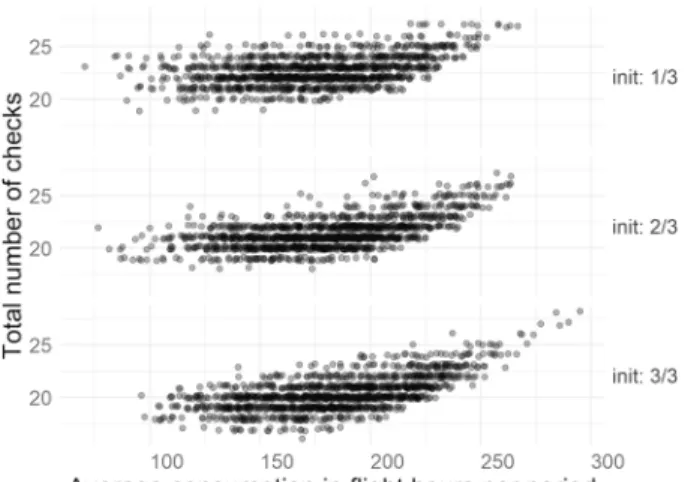
This intuition can be formalized via a supervised ML model where a response n
is a function gn(y∗) on the optimal maintenance cycle distribution (e.g., in Fig. 1 the
response is the total number of checks) and the input features are a function on the
mission flight hours demand and the fleet initial status distributions (e.g., in Fig. 1
the input feature is the average flight hour demand).
The method consists of the following. First, we choose a set of candidate responses to predict. Then, we calculate several input features that we suspect can predict those responses. Finally, after validating the ML model on said responses and input features, we obtain, for each response, the subset of input features that best
predict the chosen responses and the function that minimizes the loss function: ̂gn(x)
.
For our problem, we choose the following responses:
NM Total number of checks
𝜇T−t� Average distance between the second check and
the end of the horizon over fleet
𝜇t�−t Average distance between two checks over the fleet With the following equations:
After validating the ML model, we obtain the following input features:
𝜇C Average consumption per period
Init Sum of fleet flight hours remaining before first period Spec Sum of all special mission flight hours
𝜇WC Period that splits total consumption in two equal
parts. Can be fractional
𝜎C2 Variance of consumption per period
maxC Max consumption per period
Let the consumption in period t be represented by the following:
And let JQ represent the set of special missions, i.e., that have a capability or where Qj≠∅.
Then the equations for those input features are: NM = ∑ (i,t,t�)∈D|t�<T mitt�+ |I| 𝜇T−t�= 1 |I| ∑ (i,t,t�)∈D mitt�× (T − t�) 𝜇t�−t= 1 |I| ∑ (i,t,t�)∈D mitt�× (t�− t − M) Ct= ∑ j∈JTt HjRj t ∈ T 𝜇C= 1 �T � � t∈T Ct Init = � i∈I RftIniti Spec = � j∈JQ HjRj�TJj� 𝜇WC= ∑ t∈T Ct× t ∑ t∈T Ct 𝜎2C= 1 �T � � t∈T (Ct− 𝜇C)2 max C = maxi∈T {Ct}
7 Experimentation
Five thousand small (15 aircraft) instances are randomly generated following the
method found in Peschiera et al. (2020), which simulates French Air Force needs.
The sources of randomness are the missions, i.e., the quantity, hour needs, resource quantities, minimum durations, special requirements; and the initial fleet status, i.e., remaining calendar time, remaining flight time, special capabilities for each aircraft at the start of the planning horizon. These instances are used as an input to obtain learned constraints.
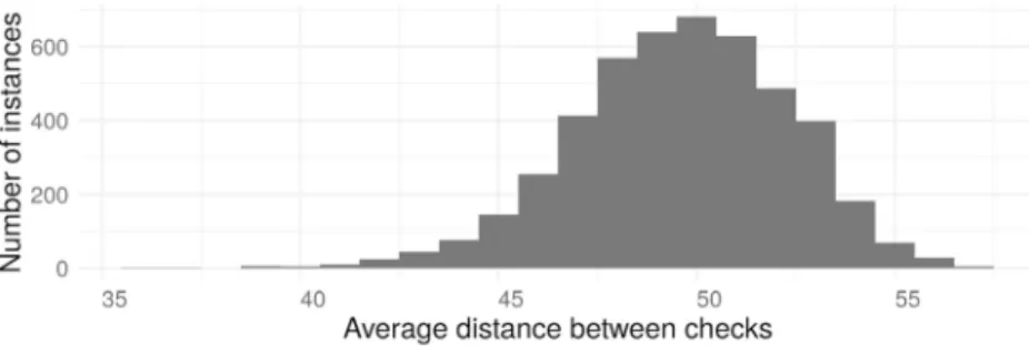
Figure 2 shows the distribution on the average distance between checks for all
solved instances.
3 additional sets of 1000 instances each are randomly generated to test the imple-mentation of these learned constraints. Each set corresponds to a particular size of fleet: 30, 45 and 60 aircraft.
In what is left of this section, we first explain mathematical model
implementa-tion and execuimplementa-tion in 7.1. We then present the statistical model implementation in
7.2. Finally, all tested mathematical models are explained in 7.3.
7.1 Mathematical model implementation
Mathematical models are generated using python 3.7 and the PuLP library. All instances are solved until optimality with a time limit of 1 hour and a tol-erance (absolute gap) of 10. We use CPLEX 12.8 running on single thread Win-dows 7 with 72 2.3GHz processors and 128 GB RAM workstation. Up to 70 experiments are run in parallel. CPLEX parameters are optimized for the problem using the CPLEX Tuner tool.
7.2 Implementation of learned constraints
The 5000 solved instances are split into two groups: training (70%) and testing (30%). The training set is used to train a statistical model. The testing set is used
for the feature selection process. Around 1000 instances are discarded in order to build the prediction model because of having violated soft constraints or having an absolute gap too large (bigger than 100). So the resulting dataset used to build the model consisted of 4084 instances.
For forecasting, we test and compare several methods: Linear Regression (LR), Decision Tree Regression (DTR), Multi-layer Perceptron regression (MLPR), Support Vector Regression (SVR), Quantile Regression (QR) and Gradient Boosted Regression Trees (GBRT).
Robust predictions involve predicting bounds, or quantiles. Only two imple-mentations offered the possibility of predicting quantiles: QR and GBRT. Both techniques are found to have similar effectiveness in predicting the 10% and 90% quantiles. At the end, the former is chosen because it returned scalar coefficients for every regressor and so is more intuitive to validate. To build the QR models,
python 3.7 is used together with the statsmodels library. Figure 3 shows the upper
bound for one of the variables ( ̂𝜇ub
t�−t).
After preliminary tests, only cuts where we assume each aircraft has a
maxi-mum deviation (tol) with respect to the mean distance between checks ( ̂𝜇t�−t ) are
found to have a positive influence in solution times:
7.3 Model experimentation
We call “base” the model described in Sect. 5, “old” the one formulated in
Peschiera et al. (2020) and “base_*” (“old_*”) the various derivatives from each
model. The model “base_determ” refers to the “base” model with deterministic
cuts added as described in Sect. 5.3.
Each learned cuts model involves the combination of two configuration param-eters, corresponding to two steps during the pattern production. In the first step, we control the maximum deviation (tol) we allow each individual maintenance pattern to be from the mean distance between maintenances prediction bounds [see Eqs.
(26) and (27)]. In the second step, we control how many of the previously rejected
maintenance patterns should we incorporate nonetheless to the model, randomly, as a percentage (recyc) of the already reduced number of patterns. The “base” model (tol = ∞ ) has no added cuts. The most aggressive model (tol = −∞ ) assumes all air-craft should have the same distance between checks, equal to the predicted average.
The notation for the learned cuts models is shown in Table 1, and they are
con-sistent between the “base” model and the “old” model.
(26) mitt�= 0 t�− t < ̂𝜇lbt�−t− tol
(27) mitt�= 0 t�− t > ̂𝜇ubt�−t+ tol
Three additional matheuristics are tested to compare the performance gains offered by the previously presented learned cuts. The matheuristics are described below:
base_flp. The linear relaxation of the “base” model is solved. Only maintenance patterns with a non-zero value in the relaxed optimal solution are kept for a second run of the “base” model.
base_flp2. The linear relaxation of the “base” model is solved. Only maintenance patterns that are similar to a pattern with a non-zero assignment (i.e., both patterns share the same aircraft and at least one date of the two checks) are kept for a second run of the “base” model.
Fig. 3 The average distance between checks in the vertical axis ( 𝜇t�−t ) vs. the sum of remaining flight
hours of the fleet at the beginning of the planning horizon (Init) in the horizontal axis for the over 4000 instances solved to optimality or close to optimality. In black are the real values from the solved instances, and in blue the predicted upper bound at percentile 90. The instances have been split in 3 equal parts, two times, according to two features: 𝜇WC in column facets and 𝜇C in row facets. “1/” corresponds
to the 33% of instances that have the lowest value for that given feature
Table 1 All learned cuts models that are based on the “base” model
Each consists of a particular combination of the tolerance for creating patterns (tol) and the percentage of random extra
pat-Model tol recyc
base ∞ 0 base_a1 2 0 base_a2 0 0 base_a3 − ∞ 0 base_a2r 0 0.2 base_a3r − ∞ 0.2
base_flp3. The linear relaxation of the “base” model is solved. Let tf i ( t
l
i ) be the soonest (latest) check for aircraft i with a non-zero value in the optimal relaxed
solu-tion. Only maintenance patterns that have the first maintenance after a tf
i and the
second maintenance before tl
i are used in the second run.
8 Results
All comparisons presented in this section, with the exception of the summary tables at the end, are done using the medium size dataset ( |I| = 30).
This section is structured as follows. First, Sect. 8.1 briefly analyses the “base”
and “old” models in terms of their performance; Sect. 8.2 presents the results of
learned cuts applied on both models; Sect. 8.3 compares the learned cuts with other
more traditional matheuristic techniques; finally, Sect. 8.4 shows a complete
com-parison including larger dataset sizes and alternative variants on the learned cuts. 8.1 Comparison between models and deterministic cuts
We compare the “base,” “old” and “base_determ” models with respect to solution time. This performance is expressed as the number of nodes that are visited in the branch and bound phase before proving optimality, the quality of the LP relaxation (before and after the cuts phase), the capacity to obtain feasible solutions and the time it takes to prove an optimal solution.
Table 2 shows statistics on the status of the solutions returned by each model.
The “old” model is considerably better at obtaining feasible solutions in less than
1 h. Table 3 shows the quality of the relaxation and the number of nodes needed to
obtain an optimal solution. The “base” model is considerably better at obtaining a good initial LP relaxation while also needing considerably less nodes to prove opti-mality. With respect to solution times to obtain an optimal solution, they present a similar performance. The deterministic “base_determ” model offers slight improve-ments on the “base” model.
8.2 Comparison of learned cuts
In order to assess the merits of the learning constraints, we use several indicators that measure three main concepts: quality degradation, performance gains and feasi-bility sensifeasi-bility.
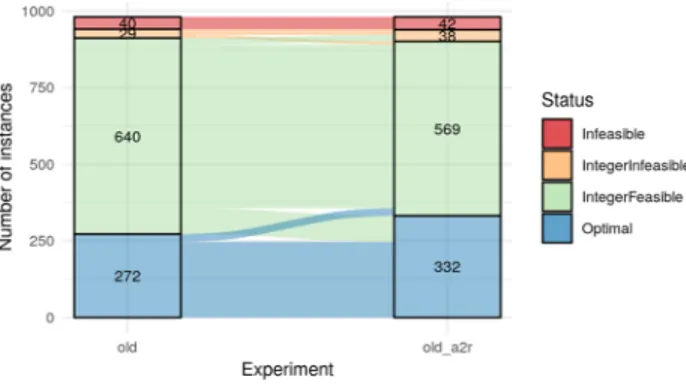
Figures 4 and 5 show a summary of the proportion and changes of the status of
the solution for both models, “base” and “old,” respectively, when applied learned cuts. The number of solutions with an “Optimal” status increases in both cases. With respect to finding feasible solutions, the “base” model sees an improvement on the number of instances without a solution (“IntegerInfeasible” status) when adding learned cuts, while the “old” model sees a regression in this respect. Note that the
number of infeasible solutions remains almost the same with the given configuration regardless of the model used.
When adding learning constraints, we eliminate valid solutions from the pool (i.e., these are invalid cuts or pseudo cuts). This implies there is a risk of taking out the actual optimal solution. In order to measure the effect of these cuts on the value of the optimal solution, we measure quality degradation as the distance (in % with respect to the “base”) between the objective functions in the cases when all models
return an optimal status. Figure 6 compares the distribution of such degradations for
each case. The degradations of the learned cuts are almost entirely lower than 5% from the “base” optimal. The “old” model is expected to have a degradation of 0% or close to 0%, which it does.
We measure the performance of each method by comparing the solution time.
Figure 7 shows the distribution of solution times for each model for all instances. It
is possible to see how adding the cuts increases performance and the greatest perfor-mance gains are obtained in the “base” model.
Table 2 Comparison of the number of instances per status returned in each model: “base”, “old” and “base_determ”
Each status is exclusive one from the other (i.e., they sum the totality of correctly generated instances). Infeasible: problem proven infeasi-ble. IntegerFeasible: an integer solution is found but not proven opti-mal before time limit. IntegerInfeasible: no integer solution is found before time limit. Optimal: difference between relaxation and best integer solution is less than the absolute gap
Indicator base base_determ old
Infeasible 41 44 40
IntegerFeasible 277 289 640
IntegerInfeasible 384 368 29
Optimal 279 280 272
Total 981 981 981
Table 3 Comparison of the quality of the linear relaxation in each model: “base”, "old" and “base_determ”
“nodes” refers to the average number of nodes needed to prove optimality, in cases where both models obtain an optimal tion. “time” is the average solution time to obtain an optimal tion. “LP_first” is the average distance (in % from the optimal solu-tion) between the initial relaxed solution and the optimal solution. “LP_cuts” is the average distance (in % from the optimal solution) between the relaxed solution after the root node cuts and the optimal solution
Indicator base base_determ old
LP_cuts 0.39 0.54 0.48
LP_first 4.93 4.91 22.04
nodes 705.32 692.60 3234.61
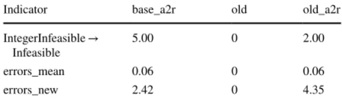
constrains violations. Table 4 shows the number of additional infeasible instances is almost non-existent, and there is very little additional instances with soft constraints violations in both models. All new infeasible instances are instances that are not proven feasible (“IntegerInfeasible → Infeasible”) and could potentially be indeed infeasible.
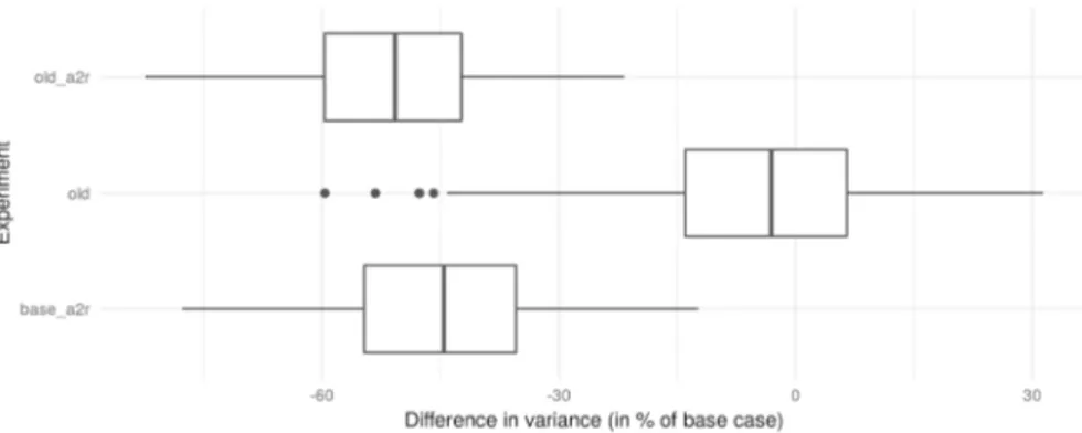
As stated previously, the uniform usage of the fleet is also a factor to take into account when choosing a correct maintenance planning. Given that the pattern selection is oriented towards constraining the check patterns that are too far from the predicted mean distance between checks, it is expected for the variance of this measure to decline. For the cases when there is more than one fleet type (i.e., for larger instances), the variances of each fleet type are calculated individually and
summed into one single indicator. Figure 8 shows how the variance is greatly
Fig. 4 Number of instances per status returned in “base” model and the changes of status when applying learned cuts. Each status is exclusive one from the other (i.e., they sum the totality of correctly generated instances). Infeasible: problem proven infeasible. IntegerFeasible: an integer solution is found but not proven optimal before time limit. IntegerInfeasible: no integer solution is found before time limit. Opti-mal: difference between relaxation and best integer solution is less than the absolute gap
Fig. 5 Number of instances per status returned in “old” model and the changes of status when applying learned cuts. Each status is exclusive one from the other (i.e., they sum the totality of correctly generated instances). Infeasible: problem proven infeasible. IntegerFeasible: an integer solution is found but not proven optimal before time limit. IntegerInfeasible: no integer solution is found before time limit. Opti-mal: difference between relaxation and best integer solution is less than the absolute gap
Fig. 6 Relative difference between the objective function value for each model, compared with the “base.” Only instances where all models return an optimal status are used. The right and left side tails representing 10% of the sample are removed for better display
Fig. 7 The distribution of solution times of each method for all instances. The x-axis represents the per-centile of instances in % from 0 to 100 and the y-axis the time it takes to solve the slowest instance in that percentile
Table 4 New infeasible instances per learned cuts model and per status in the “base” model
“IntegerInfeasible → Infeasible” is the number of additional new infeasible instances which had this status in the “base” modelz. “errors_mean” is the average of new soft constraints violations, and “errors_new” is the percentage of new instances with at least one soft constraint violation, among optimal solutions
Indicator base_a2r old old_a2r IntegerInfeasible →
Infeasible 5.00 0 2.00
errors_mean 0.06 0 0.06
8.3 Comparison with other matheuristics
Table 5 shows the extra infeasible instances for each method with respect to the
“base” model status. One can see that some previously “Optimal” and “Inte-gerFeasible” solutions in the “base” model become now “Infeasible,” in contrast with the “base_a2r” model. Also, these matheuristics introduce many more new
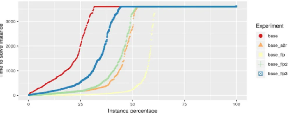
soft constraints violations. Figure 9 shows the solution time for each method
compared to the base model and to the learned cuts model: only the most aggres-sive of the matheuristics beats the previously shown learned cuts.
These two results highlight the advantage of using learned cuts over other more standard matheuristics: they offer a good combination of less degradation in new infeasible solutions and better performance in solution times.
8.4 Summary
Tables 6, 7, and 8 show a summary for each dataset of the gains and costs of
applying different degrees of cuts in models “base” and “old.” Each statistic (“Stat”) is a comparison between the named model and the “base” model. As a
Fig. 8 The percentage difference in variance for the distance between checks in alternative models with respect to the base model
Table 5 New infeasible instances per method and per status in the “base” model
e.g., 3 “Optimal” solutions in the “base” case result in “Infeasible” in “base_flp” “errors_mean” is the average of new soft constraints violations, and “errors_new” is the percentage of new instances with at least one soft constraint violation, among optimal solutions
Indicator base_a2r base_flp base_flp2 base_flp3 IntegerFeasible → Infeasible 0.00 10.00 8.00 8.00 IntegerInfeasible → Infeasible 5.00 76.00 12.00 10.00
Optimal → Infeasible 0.00 3.00 3.00 3.00
errors_mean 0.05 1.97 1.00 1.05
reference, the “old” model results are also shown and compared accordingly. It is
important to note that the “old” model is similar in feasibility ( E𝜇 , E% and Infeas),
quality degradation ( Q𝜇 , Qm and Q95 ) and variance ( V𝜇 ) as the “base” model,
since both share the same solution space. Thus, the gains in performance ( T𝜇 and
Feas), and variance reduction ( V𝜇 ) offered by the learned cuts models need to be
weighted against trade-offs on the former indicators.
Fig. 9 The distribution of solution times for each method for all 994 instances solved. In the x-axis is the percentile of instances in % from 0 to 100. In the y-axis is the time it took to solve the slowest instance in that percentile
Table 6 Summary table comparing the performance of several options of cuts in scenario of size |I| = 30
All comparisons are done against the “base” model for each option dataset size. E𝜇 and E% refer to the
percentage difference in average number of soft constraint violations per instance and the proportion of new instances with at least one violation, among optimal solutions. Feas (Infeas) refer to the average additional number of feasible (infeasible) instances obtained as a percentage of total instances (1000). Q
𝜇 , Qm and Q95 are the average, median and 95-percentile difference in the objective function when
com-Stat base_a1 base_a2r base_a3r old old_a1 old_a2r old_a3r
E𝜇 0.16 0.07 2.28 − 0.01 2.27 0.07 2.65 E% 1.02 2.54 10.66 0 10.66 4.57 13.2 Feas 25.96 32.5 33.1 36.22 32.5 35.01 35.11 Infeas 1.21 0.61 1.51 − 0.1 1.41 0.21 1.61 Q𝜇 12.97 9.86 27.65 − 0.18 56.58 6.3 14.4 Qm 2.8 3.65 8.08 0.02 6.36 2.67 5.48 Q95 4.82 7.83 11.17 0.92 9.93 4.14 7.81 T𝜇 − 16.16 − 29.5 − 49.53 0.54 − 14.17 − 5.2 − 30.39 V𝜇 − 41.31 − 42.56 − 60.19 − 1.83 − 93.2 − 48.77 − 68.45
Regarding optimality degradation (Q), solutions with cuts tend to be 5–6% away from the real optimal (or the best known solution). By recycling some excluded patterns, the gap can be reduced to less than 4%.
Regarding performance, all learned cuts increase the number of instances where a feasible solution is found in the “base” model: Feas improves by an aver-age difference of 20% to 50% (measured in % of total instances). This is not so in the case of the “old” model, where performance is lost in this sense. Gains
in solution times are also substantial. The average time ( T𝜇 ) usually improves
between 10 and 30%.
Additional infeasible solutions and soft constraints violations (Infeas and E) increase with the aggressiveness of the cuts and depending on whether we allow the possibility of recycling or not. In the cases of less aggressive cuts, most new infeasible instances are not proven feasible by the “base” model. The impact of recycling in reducing the number of infeasible instances while keeping most of the performance is to be noted.
Table 7 Summary table comparing the performance of several options of cuts in scenario of size |I| = 45
The best result for each row is shown in bold
Stat base_a1 base_a2r base_a3r old old_a1 old_a2r old_a3r
E𝜇 0 0.05 1.49 0 0.68 0.14 2.11 E% 0 2.7 10.81 0 2.7 8.11 10.81 Feas 37.01 48.55 54.56 60.58 49.55 55.07 58.48 Infeas 2 0.8 2.3 0 2.4 0.1 1.6 Q𝜇 3.14 4.54 15.68 0.37 7.39 3.73 6.48 Qm 2.8 3.77 9.2 0 7.42 2.69 5.69 Q95 6.69 10.21 24.39 1.79 11.49 9.74 15.31 T𝜇 − 8.9 − 15.48 − 31.64 0.64 − 6.62 − 1.6 − 10.65 V𝜇 − 41.62 − 45.04 − 62.71 − 2.48 − 95.29 − 48.84 − 68.16
Table 8 Summary table comparing the performance of several options of cuts in scenario of size |I| = 60
The best result for each row is shown in bold
Stat base_a2 base_a2r base_a3r old old_a1 old_a2r old_a3r
E𝜇 0 0 0 0 1.92 0 3.92 E% 0 0 0 0 7.69 0 15.38 Feas 32.59 36.02 43.18 53.88 37.23 44.7 49.44 Infeas 5.76 1.22 3.44 0.11 3.54 0.61 2.33 Q𝜇 4.57 3.97 7.74 0.63 7.13 2.54 5.28 Qm 3.97 3.15 7.47 0 6.29 2.58 5.3 Q95 8.38 7.81 13.66 3.42 14.05 4.33 9.5 T𝜇 − 10.19 − 8.26 − 18.54 0.74 − 4.48 − 0.44 − 5.67 V𝜇 − 50.9 − 43.28 − 61.98 1.13 − 94.89 − 47.54 − 66.8
Finally, variance reduction (V) between 40 and 60% is usually obtained with most cut strategies, although recycling reduces slightly the strength of the reduction. The more aggressive a cut, the most the gain in variance reduction.
Larger instances allow for more aggressive cuts without losing too much feasibil-ity or qualfeasibil-ity, as can be seen by comparing the impact of “base_a3r” across different sizes of instance. The cuts in the “base” model have greater reductions in solution time than those in the “old” model, while the cuts in the latter have slightly lower feasibility and quality degradation and slightly greater variance reductions. This can be explained as the nature of the cuts differs in each formulation: in the “base” model it consists of reducing the number of variables, while in the “old” model it consists of adding constraints.
The best compromise seems to be reached when adding recycling to aggressive cutting (“base_a2r” or “base_a3r”) depending on the size of the instance. In most of the cases, a low or very low optimality degradation can be seen together with a low feasibility change, compared to both the “base” and “old” models. The performance gains can be seen in both time to reach an optimal solution and the reduction of the variance of the usage of the fleet. Finally, compared to the “base” model, the amount of feasible solutions is increased.
These results encourage the design of more sophisticated ways of predicting terns in solutions. Ideally, a function that returns a probability distribution of pat-terns for each instance could be trained and then used to sample promising patpat-terns. Our learned cuts model is a special case where we give a very high priority (a prob-ability of 1) to patterns in the range of tolerance for the distance between checks and a very low probability (dependent on the recycling parameter and the total amount of available patterns) to the rest of the patterns.
9 Conclusions
This paper presents an alternative MIP formulation for the long-term Military Flight and Maintenance Planning problem. The performance is compared with previous formulations using cases inspired by the French Air Force. Valid bounds are for-mulated and tested. A forecasting model is designed to predict characteristics of optimal solutions based on the input data and used to create pseudo-cuts. For com-parison, several matheuristic that use the LP relaxation are also applied to reduce the solution space of the problem.
The study shows that predicting characteristics of the optimal solution is a power-ful method to obtain very good solutions that are close to the optimal, in less time and with very little loss of feasibility. In addition, the prediction also allows con-sideration of a second objective without hindering performance. The performance gains of these pseudo-cuts will depend heavily on the implementation, i.e., on the mathematical model employed and the way the pseudo-cuts are added to the model.
Further work includes, first of all, researching better ways to predicting the optimal patterns in a solution. Secondly, the application of this technique into problems where pattern can potentially be used, such as workforce scheduling and cutting stock problems. Furthermore, this technique can be generalized into a random sampling of patterns where each pattern is picked with a probability equal to the potential it has to appear in the optimal solution.
Funding This paper was written as part of a PhD Thesis partially financed by the French Defense Pro-curement Agency of the French Ministry of Defense (DGA).
Appendix A: Time‑related index sets
Consider a small example where M = 2, RctInit
1 = 5, E max = 7, Emin = 4, MTmin 1 = 3, MT max
1 = 4, T = 15, T1 = {4, … , 10}, Ji=1 = {1} ; then, the example
solution in Fig. 10 should comply with the following:
TMInit
i =
{
t ∈{max {0, RctInit
i − E
max+ Emin}, … , RctInit
i }} . Ts t� = { t ∈{max {1, t�− M + 1}, … , t�}} . TM t� = {
t ∈ {t�+ M + Emin− 1, … , t�+ M + Emax− 1} ∩ {T − Emax+ 1, … , T − 1}}.
TM+t� = { TMt�. t�+ M > T ∨ t�+ M + Emax− 1 < T TM t� ∪ {T}. t �+ M ≤ T ≤ t�+ M + Emax− 1 T T Tt= {(t1, t2) ∣ t1∈ T s t∨ t2∈ T s t}. T Tj= {t, t�∈ T j∣ t + MT min j − 1 ≤ t �≤ t + MTjmax− 1}. T T Jjt= {t1, t2∈ T Tj∣ t1≤t ≤ t2}. JT Tit 1t2 = {(j, t, t �)|j ∈ J i∧ (t, t �) ∈ T T j∧ t ≥ t1+ M ∧ t � <t2}.
Fig. 10 The figure shows an example solution that complies with the time-related indexed sets. Air-craft 1 has a first check in period 2 ∈ TMInit
1 . A second check is done in period 9 ∈ T
M
2 . Also, since
(2, 9) ∈ T T T3 , aircraft 1 is considered in maintenance in period 3. The aircraft has an assignment to
mission 1 in periods (5, 8) ∈ T T1 . Since (5, 8) ∈ T T J15 , aircraft 1 is considered assigned to mission 1
during period 5. Finally, since maintenances are done in periods (2, 9), all possible mission assignments in between (e.g., (1, 5, 8)) should be in JT T129
References
Achterberg T, Koch T, Martin A (2005) Branching rules revisited. Oper Res Lett 33(1):42–54. https ://doi. org/10.1016/j.orl.2004.04.002
Adamo T, Ghiani G, Grieco A, Guerriero E, Manni E (2017) MIP neighborhood synthesis through semantic feature extraction and automatic algorithm configuration. Comput Oper Res 83:106–119 Adamo T, Ghiani G, Guerriero E, Manni E (2017) Automatic instantiation of a variable neighborhood
descent from a mixed integer programming model. Oper Res Perspect 4:123–135
Aghezzaf EH, Najid NM (2008) Integrated production planning and preventive maintenance in deterio-rating production systems. Int J Prod Econ. https ://doi.org/10.1016/j.ins.2008.05.007
Bello I, Pham H, Le QV, Norouzi M, Bengio S (2016) Neural combinatorial optimization with reinforce-ment learning. arXiv preprint arXiv :1611.09940
Bengio Y, Lodi A, Prouvost A (2018) Machine learning for combinatorial optimization: a methodological tour d’Horizon. arXiv :1811.06128
Cho P (2011) Optimal scheduling of fighter aircraft maintenance. Ph.D. thesis, Massachusetts Institute of Technology
Cochran JJ, Cox LA, Keskinocak P, Kharoufeh JP, Smith JC, Fischetti M, Lodi A (2011) Heuristics in mixed integer programming. In: Wiley encyclopedia of operations research and management sci-ence. Wiley, Hoboken. https ://doi.org/10.1002/97804 70400 531.eorms 0376
De Chastellux P (2016) Planification de la maintenance des avions de chasse. Master’s thesis, ENSTA ParisTech
Department of the Army (2017) Headquarters: army aviation maintenance. Tech. rep. https ://rdl.train .army.mil/catal og-ws/view/100.ATSC/574C5 86C-A989-425A-9F3C-C92C6 93D92 3F-15052 23206 762/atp3_04x7.pdf. Accessed 18 Sept 2019
Dupin N, Talbi E (2018) Parallel matheuristics for the discrete unit commitment problem with min-stop ramping constraints. Int Trans Oper Res 27(1):219–244. https ://doi.org/10.1111/itor.12557
Fischetti M, Fraccaro M (2019) Machine learning meets mathematical optimization to predict the opti-mal production of offshore wind parks. Comput Oper Res 106:289–297. https ://doi.org/10.1016/J. COR.2018.04.006
Fischetti M, Glover F, Lodi A (2005) The feasibility pump. Math Program 104(1):91–104. https ://doi. org/10.1007/s1010 7-004-0570-3
Gavranis A, Kozanidis G (2015) An exact solution algorithm for maximizing the fleet availability of a
TMInit 1 = {2, … , 5} Ts 3 = {2, 3} TM 2 = {7, … , 10} TM 7 = {12, … , 14} TM+ 9 = {14, 15} T T T3 = {(2, 7), … (2, 10), (3, 8) … (3, 11)} T T1 = {(4, 6), (4, 7), (5, 7), (5, 8), … , (8, 10)} T T J15= {(4, 6), (4, 7), (5, 7), (5, 8)} JT T129= {(1, 4, 6), (1, 4, 7), (1, 5, 7), (1, 5, 8), (1, 6, 8)}