HAL Id: hal-01327787
https://hal.archives-ouvertes.fr/hal-01327787
Submitted on 7 Jun 2016HAL is a multi-disciplinary open access
archive for the deposit and dissemination of sci-entific research documents, whether they are pub-lished or not. The documents may come from teaching and research institutions in France or abroad, or from public or private research centers.
L’archive ouverte pluridisciplinaire HAL, est destinée au dépôt et à la diffusion de documents scientifiques de niveau recherche, publiés ou non, émanant des établissements d’enseignement et de recherche français ou étrangers, des laboratoires publics ou privés.
Elimination at the Final Point
Natalia Varminska, Damien Chablat
To cite this version:
Natalia Varminska, Damien Chablat. Optimal Motion of Flexible Objects with Oscillations Elimina-tion at the Final Point. New Trends in Mechanism and Machine Science. Mechanisms and Machine Science, Springer, Cham, pp.281-291, 2016, 978-3-319-44155-9. �10.1007/978-3-319-44156-6_29�. �hal-01327787�
1
Optimal Motion of Flexible Objects with
Oscillations Elimination at the Final Point
Natalia Varminska and Damien Chablat
1
Sevastopol State University, Russian, e-mail: [email protected]
2
IRCCyN, CNRS, France e-mail: [email protected]
Abstract. In this article, a theoretical justification of one type of skew-symmetric optimal translational
motion (moving in the minimal acceptable time) of a flexible object carried by a robot from its initial to its final position of absolute quiescence with the exception of the oscillations at the end of the mo-tion is presented. The Hamilton-Ostrogradsky principle is used as a criterion for searching an optimal control. The data of experimental verification of the control are presented using the Orthoglide robot for translational motions and several masses were attached to a flexible beam.
Key words: Motion planning, Oscillations, Parallel robot, Orthoglide.
1.
Introduction
Considering the flexible object moving requirements and the robotic industrial needs, the most important one is the evaluation and the possible suppression of the robots oscillations or the oscillations of the objects which the robots move. Actu-ally, robots with reduced structure masses are appeared and as a result they lose the structural rigidity thus affecting the system dynamics. Use of structures and materials that can suppress the oscillations is quite expensive and furthermore not fully acceptable [1, 2]. Additional approaches based on software solutions need a calibration of the control loop and a specific path planning phase to decrease the positioning errors [2 – 4].
The trajectory planning of a robot generally means developing a mathematical algorithm for the selection and the description of the desired motion between the initial and the final points of the trajectory. To do this, two approaches are usually used [5 – 8]. In the first one, the exact set of constraints (for example, continuity and smoothness of the functions) on the position, velocity and acceleration of the generalized coordinates of the robot in some points of the trajectory are specified. Then the planner selects the trajectory that passes through the needed points and satisfies the given constraints into them from a class of functions (for example, among the polynomials). The trajectory developed by the planner must take into consideration the mechanical constraints of the robot and, hence, a smooth trajec-tory has to be searched. To satisfy this demand, it would be desirable to get the
trajectories with continuous functions of the joint accelerations, so that the jerk stays limited. The restrictions definition and planning of the trajectory are per-formed in the joint space. In the second one, the desired trajectory of the robot is described as an analytic function, for example, a linear trajectory in Cartesian workspace. The planner makes an approximation of the desired path in Cartesian or joint coordinates. The trajectory planning in joint variables has several ad-vantages: a) there is the definition of the variables directly controlled during the motion; b) trajectory planning can be performed in real-time; c) trajectory plan-ning in joint coordinates is easier to execute. The drawback is the complexity to determine the position of robot links and the end-effector during the motion. The same tendency can be noted for moving flexible objects. Trajectory planning tech-niques aim at the minimization of some objective functions that usually are the implementation time, the actuator efforts and the jerk [6, 9, 10, 12]. Due to the need to increase productivity in industry, the first used trajectory planning tech-nique is the minimum time algorithm [11 – 14]. The main drawback of these ap-proaches is that the generated trajectories have discontinuous accelerations and the joint torque values and they bring in the dynamic difficulties in the trajectory im-plementation. Some robot trajectory planning algorithms with power criterions are employed, for example, in [6, 7, 12, 15].
The next algorithm provides a jerk-optimal trajectory by minimizing the jerk value during the trajectory performance. According to the algorithm, the position-ing errors, the actuators stresses and the robot structures (i.e., definition of the res-onance frequencies) can be detected in [16, 17]. While planning the trajectory of a flexible object, a manipulator can move with the object slowly enough to respond to the velocity and torque constraints [18 – 20]. In these papers, the motion is di-vided into three phases: a motion with acceleration, a motion with constant veloci-ty and the deceleration. The first phase lasts until the velociveloci-ty boundary is achieved, then the constant-velocity phase starts. In proposed method the torque, dynamic and kinematic constraints are satisfied and the needed object position and velocity can be reached at the end point. In [18], it was presented a trajectory planning approach that satisfies the dynamic constraints (the torque and the ve-locity constraints) and in this way the position and the veve-locity conditions at the final point could be satisfied both. In the paper the authors proposed to set apart the task of planning the direction of a robot and the task of the speed-planning. There are studies on the control of oscillations of linear and nonlinear mechanical systems in absolute motion [21, 22]. In [23, 24], the authors focus on optimal con-trol of translational and rotational motions of the flexible systems with finite or in-finite number of degrees of freedom. When transporting in a minimal time of non-rigid objects or moving a robot with limited non-rigidity, the oscillations of the robot and these transported objects occur. But the dynamics of non-rigid robots in opti-mal translational motion deserves special attention. Research of the optiopti-mal mo-tion control of the flexible objects with the eliminamo-tion of oscillamo-tions at the end of the motion is required. The control tasks of flexible systems are relevant in using robots with finite rigidity (robots of minimal mass), transportation and assembly
3
of the flexible objects under terrestrial conditions and in outer space. There is a need to use such special motion controls, in which oscillations of transported ob-jects are significantly reduced or completely eliminated, i.e. in an acceptable min-imum possible time of translational motion the relative or absolute quiescence at the end of the movement is achieved [25, 26]. The proposed motion control pro-vides moving a flexible object (or a non-rigid robot arm) from the initial position of absolute quiescence to the end position of absolute quiescence with oscillation acceptability only during the motion and elimination of them at the end point. So there is no positioning accuracy loss. The functions describing the positions, the velocities and the accelerations in translational motion are smooth and they are functions of the object natural frequency and motion time. The total motion time also depends on the object natural frequency.
This paper is composed in the following way. The first section gives theoretical justification of an optimal translational motion using the Hamilton-Ostrogradsky principle. The next section deals with the experimental verification of this motion. Here the results of practical investigation of the flexible object motions with dif-ferent masses are presented. Finally, the conclusions are made and a future re-search is presented.
2.
Theoretical justification of an optimal
transla-tional motion
A flexible object participates in two motions: a translational or rotational mo-tion, (this is a motion with the moving coordinate system) and the relative motion (this motion is relative to moving coordinate system, i.e. oscillations). The Hamil-ton-Ostrogradsky principle can be used as a criterion for searching an optimal con-trol of translational motions of flexible objects [27]. This motion can be optimal in the sense of some optimality criterion (which can be known before or should be found as a result of research). The possibility of using the Hamilton-Ostrogradsky principle (in the Lagrange form) as a criterion for the motion optimality of the rig-idly-flexible frames employing a pulse force is considered in [28]. In [29] it is shown that the dry friction in studying the natural oscillations can be considered as a relay control which is found using the Pontryagin maximum principle on the ba-sis of the time criterion or the action principle.
For justification of the optimal control, the Hamilton-Ostrogradsky principle is involved and it means that for the non-conservative (controlled) system,
(
)
1 0 t e J=∫
T− Π +A dt, (1) the action takes a stationary value in real (true) motion. For example, for a sys-tem with one degree of freedom the kinetic energy of the translational motion at any moment of time is 22,
e
translational velocity at any moment of time. The potential energy stored during the optimal fast translational motion of the flexible object is 2 2
2
e
П сs= n , where
c is the rigidity coefficient; se is the translational displacement at any moment of
time; n=t1 tc, where t1 is the total motion time; tc is the period of the natural
os-cillations of an object (in relative motion). Essentially, using n takes into account the deformation of the flexible object due to the translational motion. The higher the natural frequency k of oscillation of an object
(
tc=2 /π k)
, i.e. the higher rigid-ity of the flexible connection, the less potential energy of deformation stored as a result of the fairly rapid translational motion.The mechanical work of the control force at any moment of time is е *
e e А u s= , where • * * 2 e e u =ms p , and s*e=V tср =Lt t1; p k n= ;
• L is the overall displacement of an object during the motion t1;
• Vcp = L / t1 is average speed.
After substituting in Eq. (1), the criterion takes the form:
1 2 2 3 2 0 2 2 2 t e e e mv cs mLp J ts dt n π = − +
∫
. (2)For the functional (2) that for this case in the general form is written as
(
)
1 0 , , , t e e F s s t dt∫
the Euler equation is
0 e e s s d F F dt − = .
After transformations for m = 1, we receive
2 3 2 2 2 . e e d s Lp p s t dt + = π (3)
The solution of Eq. (3) with the initial conditions se(0) 0 = and (0)se =ve(0) 0= is:
( )
(
)
( ) sin 2 e L s t pt pt π = − ,and then the velocity and acceleration are:
( )
(
)
( ) ( ) 1 cos ; 2 e e Lp v t s t pt π = = − ( ) ( ) 2sin( )
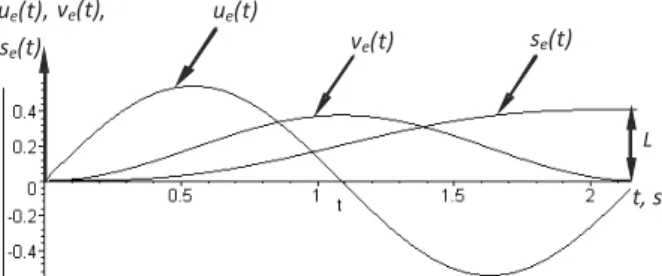
2 e e Lp u t v t pt π = = (4)Functions se(t), ve(t) and ue(t) for initial data: L= 0.41 m, k= 5.78 s-1 and p= k / n
5 t, s ue(t), ve(t), se(t) L ue(t) ve(t) se(t)
Figure 1. Translational motion graphs: se(t) displacement, ve(t) velocity, ue(t) acceleration
They satisfy the boundary conditions of the translational motion ue(0) 0= ,
1
( ) 0
e
u t = , (0) 0ve = , (0) 0se = and the following additional conditions at the right
end, which can be represented as the moment ratios:
1 1 0 0 ( ) 0; ( ) . t t e e u t dt= v t dt=L
∫
∫
The oscillator differential equation in the relative motion (oscillations) is
( )
2 2 ( ) ( ) sin 2 r r Lp x t k x t pt π + = − and its solution with zero initial conditions
(
xr(0) 0,= xr(0) 0=)
is as follows,(
)
( )
( )
2 2 2 ( ) sin sin . 2 r Lp p x t kt pt k k p π = − − t, s xr, vr,ar, xr vr arFigure 2. Relative motion graphs: xr displacement, vr velocity, ar acceleration
Then the velocity and acceleration in relative motion are:
(
)
(
( )
( )
)
3 2 2 ( ) cos cos , 2 r Lp v t kt pt k p π = − −(
)
(
( )
( )
)
3 2 2 ( ) sin sin 2 r Lp a t p pt k kt k p π = − −Figures 1 and 2 show that at the end point of the displacement, velocity and ac-celeration in relative motion are equal zero. Thus the velocity and acac-celeration in translational motion is equal to zero and the displacement is equals to L. So there is the position of absolute quiescence with needed displacement. The moment
ra-tios at the right end, which mean that relative displacement and velocity equal zero at t = t1, are written 1 1 0 0 ( ) cos( ) 0; ( ) sin( ) 0. t t e e u t kt dt= u t kt dt=
∫
∫
(5)The relations (5) with accounting (4) and р = k / n, t1 = 2π / p are transformed in
transcendental equations:
(
)
(
)
сos 2nπ − =1 0, sin 2nπ = 0. (6) Equation (6) with the exception of the resonance has a solution: n = 2, 3,… . Found n is used to calculate the total motion time t1. It should be noted that it
could be found n for which during the time t1 a flexible object moves from the
ini-tial to the final state for all skew-symmetric controls for which is true
1 0 ( ) 0, t e u t dt=
∫
ue(0) 0 and ( ) 0= u te 1 = .3.
Experimental verification of the optimal
transla-tional motion
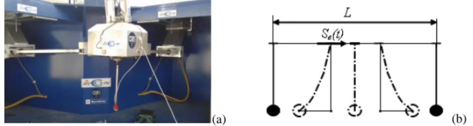
So, there was made an experiment of the optimal translational motion of a flex-ible beam from an initial point to the final point in a minimal time that is con-sistent with the natural frequency of the beam. The experiment was made in the IRCCyN’s laboratory using the Orthoglide 5-axis robot (Figs 3 a) [30, 31] built by Symetrie (France) and following equipment: an accelerometer of series FA 101 (FGP Instrumentation) and DS1103 PPC Controller Board. The trajectories of the robot were calculated using Matlab and supplied to the DS PPC Controller Board card. The actuator positions are acquired with a frequency equal to 9 kHz but the robot motions are controlled thanks to a sub program working at 1.5 kHz. As the position information transits the drives which perform the encoder emulation. Noise on the position and speed appears even when the robot is stopped. The am-plitude of this noise is about four micrometers.
The oscillator's base is clamped in the chuck of milling of the Orthoglide 5-axis robot. It moves under the influence of the control function u te( )=asin
( )
pt with time agreed with the first period of the oscillations of the flexible system (Fig. 3b). This system is a beam with a rectangular cross-section (with l= 0.305 m, b= 0.013 m, h= 0.5·10-3 m and Young's modulus E= 2.1·1011Pa) and with a mass located at its tip. The graphs of the oscillations of the object obtained with the accelerometer (for initial data: L= 0.41 m, m= 0.09 kg and k= 5.78 s-1) are given in the Figs. 4 without filtering and 5 with filters. Filtering is needed to cut off high pass fre-quencies (noise) in the signal which are produced by the accelerometer. For this purpose, here, a Butterworth filter is used. This is a type of signal processing filter
7
organized to get a frequency response as flat as possible in the passband. The But-terworth filter rolls off more slowly around the cutoff frequency than the Cheby-shev filter or the Elliptic filter but it has no ripple. And zero-phase filter helps to save features in a filtered time waveform exactly where they occur in the unfil-tered signal.
(a) (b)
Figure 3. a) scheme of the experiment using semi-industrial prototype of the Orthoglide 5-axis; b) scheme of the movement of an object with one degree of freedom
[s] [m]
[s] [m]
Figure 4. Oscillations of the object tip for m= 0.09 kg without filtering
Figure 5. Oscillations of the object tip for
m= 0.09 kg with filtering
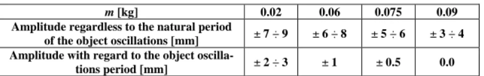
For the experiments, a 4th order Butterworth filter was used with the following pa-rameters of the filtering: the band pass filter is [0 : 20]Hz and hence the cut-off frequency is 20 Hz. The graphs confirm the absence of the oscillations at the end of the motion but in the graphs it could be noticed a ‘‘measurement noise’’ before and after measuring. If the motion time is calculated regardless to the first period of the object oscillation, there are significant displacements at the end of the mo-tion even if the momo-tion time is bigger (Fig. 6). For this case, the amplitude is ± 3 ÷ 4 mm. There were obtained the oscillation graphs for a mass m= 0.06 kg (Fig. 7 and 8). Here, it could be seen that the oscillations are significantly decreased but not eliminated at all. It can be explained by the inaccuracies in initial data of ex-periment. But elimination of the oscillations could be reached by using control feedback.
In the first case, the amplitude of the oscillations (with regard to the natural period of the oscillations) is ±1 mm at the object tip and, in the second case (regardless to the object oscillations period), the amplitude is ± 6 ÷ 8 mm. So, for this one, using the proposed motion control allows to decrease the oscillations almost 6 times.
The experiments are also made with the following masses 0.02 kg, 0.075 kg and 0.15 kg. In all cases, we observe the same behavior of the system. The results are presented in the table 1.
[s] [m]
Figure 6. Oscillations of the object tip for m= 0.09 kg
[s] [m]
[s] [m]
Figure 7. Oscillations of the object tip for
m = 0.06 kg
Figure 8. Oscillations of the object tip for
m = 0,06 kg regardless to its first period
TABLE I. AMPLITUDE OF THE OSCILLATIONS OF THE OBJECT TIP
m [kg] 0.02 0.06 0.075 0.09
Amplitude regardless to the natural period
of the object oscillations [mm] ± 7 ÷ 9 ± 6 ÷ 8 ± 5 ÷ 6 ± 3 ÷ 4 Amplitude with regard to the object
oscilla-tions period [mm] ± 2 ÷ 3 ± 1 ± 0.5 0.0
The energy expenditure for the operations performance was estimated. For ex-ample, for an object mass m= 0.09 kg changing the motion time by 5 % produces the 12 ÷ 18 % energy drop. For an object mass m = 0.06 kg changing the motion time by 10 % entails the energy costs by 60 ÷ 70 %.
4.
Conclusions
It was proved during the experiment that only increasing the motion time does not remove the oscillations of the flexible system but use of the proposed control and choosing the motion time depending on an object natural frequency eliminate the oscillations at the end point. Nowadays, the implementation of the necessary precise time for the technological operations of the object movements is a simple
9
task for the majority of industrial robots. So it is convenient to use the proposed motion control, as it saves energy 1.5 ÷ 2 times (depending on the object mass). The suggested control may be effectively used to eliminate the oscillations of the flexible systems or to decrease them 3 ÷ 10 times (depending on the object mass and motion time) during the transporting operations, the assembly of flexible ob-jects under terrestrial conditions or in outer space. In future works, it is planned to take into account the dry and the linear-viscous resistances in the object motions and investigate the motions from non-zero initial conditions.
Acknowledgements The work presented in this paper was partially funded by
the Erasmus Mundus project “Active”. Both authors also thank A. Jubien, E. Besnier and P. Lemoine for their technical assistance during the experiments.
5.
References
1. Shalymov S.V., 2003, Damping of Oscillation of Linearly Damped Elastic Sys-tem by Controlling the Stiffness, Proc. of the universities, J. of Instrumentation, Vol. 5, pp. 36-42.
2. Krutko P.D., 2003, Oscillation control, Journal Theory and Control Systems, Izvestiya RAN, Vol. 2, pp. 24 – 41.
3. Gasparetto A., Lanzutti A., Vidoni R., Zanotto V., 2011, Validation of Minimum Time-Jerk Algorithms for Trajectory Planning of Industrial Robots, Journal of Mechanisms and Robotics, Vol. 3, p. 031003.
4. Barre P. J., Bearee R., Borne P., Dumetz E., 2005, Influence of a Jerk Controlled Movement Law on the Vibratory Behaviour of High-Dynamics Systems, J. Intell. Rob. Syst., 42(3), pp. 275 – 293.
5. Gasparetto A., Boscariol P., Lanzutti A., Vidon R., 2012, Trajectory Planning in Robotics, Mathematics in Computer Science, pp. 359 – 369.
6. Voronov A.A., 1992, Automatic Control Theory of Nonlinear and Special Sys-tems, Nauka, Moscow, 288 p.
7. Gorobetc I.A., 2001, Industrial Robotics. Manipulators Mechanical Systems, Do-netsk.
8. Egorov A.I., 2004, Control Theory, Fizmalit, Moscow.
9. Siciliano B., Sciavicco L., Villani L., Oriolo G., 2009, Robotics. Modelling, Planning and Control, 2nd ed., Springer-Verlag New York, Inc. Secaucus, NJ, USA, 632 p.
10. De Schutter, J., 2010, Invariant Description of Rigid Body Motion Trajectories, ASME J. Mech. Rob., Vol. 2, p. 011004.
11. Constantinescu D., Croft E. A., 2000, Smooth and Time-Optimal Trajectory Planning for Industrial Manipulators along Specified Paths, J. Rob. Syst., 17(5), p. 233-249.
12. Besekersky V.A., 2003, Theory of Automatic Control Systems, Professiya, SPb, 752 p.
13. Melnichuk P.P., Samotokin B.B., Polishchuk M.N., 2005, Flexible computerized systems: design, modeling and control, Zhitomir, 785 p.
14. Matviychuk A.R., 2004, The Task of Optimal Minimal Time Control of the Ob-ject on the Plane with Phase Constraints, Journal of Theory and Systems of Con-trol, Izvestiya RAN, Vol. 1, p.89 – 95.
15. Saramago S.F.P., Steffen V., 1998, Optimization of the Trajectory Planning of Robot Manipulators Tacking into Account the Dynamics of the System, Mech. Mach. Theory, 33(7), pp. 883–894.
16. Piazzi A., Visioli A., 2000, Global Minimum-Jerk Trajectory Planning of Robot Manipulators, IEEE Trans. Ind. Electron., 47(1), pp. 140 – 149.
17. Lombai F., Szederkenyi G., 2009, Throwing Motion Generation Using Nonlinear Optimization on a 6-Degree-of-Freedom Robot Manipulator, Proceedings of IEEE International Conference on Mechatronics.
18. Chwa D., Kang J., Choi J.Y., 2005, Online Trajectory Planning of Robot Arms for Interception of Fast Maneuvering Object Under Torque and Velocity Con-straints, IEEE Transactions on Systems, Man and Cybernetics, Systems and Hu-mans, Vol. 35, No. 6, pp. 831 – 843.
19. Cao B., Dodds G.I., 1996, Implementation of Near-time-optimal Inspection Task Sequence Planning for Industrial Robot Arm, Proc. IEEE Int. Workshop Ad-vanced Motion Control, Mie, Japan, Vol. 2, pp. 693 – 698.
20. Munasinghe S. R., Nakamura M., Aoki S., Goto S., Kyura N., 1999, High Speed Precise Control of Robot Arms with Assigned Speed under Torque Constraint by Trajectory Generation in Joint Coordinates, Proc. IEEE Int. Conf. Systems, Man and Cybernetics, Tokyo, Japan, Vol. 2, pp. 854 – 859.
21. Chernousko F.L., Akulenko L.D., Sokolov B.N., 1980, Oscillations Control, Nauka, Moscow, 384 p.
22. Karnovsky I.A., Pochtman Y.M., 1982, Oscillations Optimal Control Methods for Deformable Systems, Vischa shkola, Kyiv, 116 p.
23. Bokhonsky A.I., Varminska N.I., 2014, Reverse Principle of Optimality in Con-trol Tasks of Translational Motion of Deformable Objects, Vestnik SevNTU, Journal of Mechanics, Energetics, Ecology, Sevastopol, pp. 130 – 134.
24. Bokhonsky A.I., 2013, Actual Problems of Variational Calculation, Palmarium Academic Publishing, Deutschland, 77 p.
25. Bokhonsky A., Buchacz A., Placzek M., Wrobel M., 2011, Modelling and Inves-tigation of Discrete-Continious Vibrating Mechatronic Systems with Damping, Wydawnictwo Poitechniki, Gliwice, 171 p.
26. Bokhonsky A.I., Varminska N.I., 2012, Optimum Braking of Flexible Object, Se-lected engineering problems, Vol. 3, Silesian University of Technology, Gliwice, 220 p.
27. Bokhonsky A.I., Varminska N.I., 2012, Variational and Reversing Calculus in Mechanics, Sevastopol, 212 p.
28. Bokhonsky A.I., Buzanova O.P., 1977, Optimal Design of Rigidly-Flexible Frames under Seismic Influence, Journal of Strength of Materials and Structures Theory, pp. 64 – 69.
29. Bokhonsky A.I., Isaeva E.V., 2004, Analysis of a Rigid Body Motion with Dry Friction, Vestnik SevSTU, Journal of Physics and Mathematics, Sevastopol, pp. 115 – 121.
30. Caro S., Chablat D., Lemoine P., Wenger P., 2015, Kinematic Analysis and Tra-jectory Planning of the Orthoglide 5-axis, IDETC and Computers and Infor-mation in Engineering Conference, Boston, USA.
31. Chablat D., and Wenger P., “Architecture Optimization, of a 3-DOF Parallel Mechanism for Machining Applications, The Orthoglide,” IEEE Trans. on Robot-ics and Automation 19, 2003, pp.403410.