A simple method to determine the diffusivity of green wood

Texte intégral

(1)PEER-REVIEWED ARTICLE. bioresources.com. A Simple Method to Determine the Diffusivity of Green Wood Rémy Frayssinhes,* Stéphane Girardon, Bertrand Marcon, Louis Denaud, and Robert Collet Log temperature appreciably influences veneer quality during the rotary peeling process. The assessment of the thermal properties of green wood is complex and typically requires the sawing of small calibrated samples. This study introduced a simple approach based on an inverse identification method to determine the global log thermal diffusivity online and without the time-consuming extraction of wooden samples that is commonly used to perform diffusivity experiments. This method was applied to green Douglas fir logs and resulted in an average thermal diffusivity of 0.175 ± 0.021 mm2.s-1. This method was found to be suitable for both heartwood and sapwood and thus can provide a globally applicable diffusivity assessment method. This global parameter is essential to optimizing the soaking time and improving the subsequent veneer production quality. As log-soaking preprocessing requires an immense input of energy, this timeoptimization strategy will allow sizable cost reduction and ecological improvement. Keywords: Green wood; Thermal diffusivity; Douglas fir; Soaking temperature; Rotary peeling preprocessing Contact information: Arts et Metiers Institute of Technology, LaBoMaP, HESAM Université, 71250 Cluny, France; *Corresponding author: Remy.Frayssinhes@ensam.eu. INTRODUCTION The temperature of logs during the rotary peeling process substantially affects veneer properties (Hecker 1995; Aydin et al. 2006; Dupleix et al. 2013; Rohumaa et al. 2016), such as mechanical strength, surface roughness (Corder and Atherton 1963; Frayssinhes et al. 2019), and also knife service life. Most industrial wood peeling operations rely on an empirical method to adjust the soaking conditions in terms of temperature and time, and those setting are rarely optimized with the possible huge variability of the supply (diameters, wood quality…). This study focused on the kinetics of temperature change inside a log that was soaked at a given target temperature with a given homogeneous initial temperature, which resulted in the best veneer quality in the shortest time. The initial log temperature can range from -10 °C to 30 °C at the log storage area, depending on outside weather circumstances (seasons). Both high moisture content and a particular homogeneous temperature are necessary for efficient cutting (Thibaut 1988). The thermal diffusivity of greenwood is a key parameter for estimating the temperature in any part of the log volume (in particular, at the geometrical center) based on soaking duration. Thermal diffusivity (𝛼) is defined as the ratio of the considered material conductivity (𝜆) to its density (𝜌) and its specific heat capacity (𝐶𝑝 ). The green wood diffusivity is different from that of the dry wood due to the different moisture content, which modifies the water proportion inside the material. Therefore, thermal conductivity, density, and global specific Frayssinhes et al. (2020). “Green wood diffusivity,”. BioResources 15(3), 6539-6549.. 6539.

(2) PEER-REVIEWED ARTICLE. bioresources.com. heat capacity are impacted, but not to a similar extent. The thermal diffusivity is commonly expressed in m2.s-1 (S.I. units) or in mm2.s-1. Several methods have been developed over the years to determine the wood thermal diffusivity, as for other materials; hereinafter are listed some of these experimental techniques. The guarded hot plate method (ISO 8302) is among the early methods to quantify the thermal conductivity of a material. Sonderegger et al. (2011) used this method to determine the conductivity and diffusivity of Norway spruce and European beech from oven-dry to 20% of moisture content. Transient hot strip (THS) techniques (ASTM D7896-14) can provide values for conductivity (𝜆) and diffusivity (𝛼) from the temperature measured locally, by a thermocouple, sandwiched between two specimens. The flash method (Parker et al. 1961), another transient technique, can provide diffusivity (𝛼) values from the temperature change, on the rear face of a sample exposed to a laser or a lamp, that supplies heat through the front face. A thermocouple, or an infrared camera, which provides the whole temperature field on the rear face of the sample, can measure the local temperature changes. The transient plane source techniques (TPS, ISO 22007-2) used by Dupleix et al. (2012) can provide value for conductivity (𝜆) and diffusivity (𝛼) by fitting the TPS experimental results with the analytical models presented by Gustafsson (1991), leading to the conductivity (𝜆) and the diffusivity (𝛼) values. Maku (1954) studied thermal diffusivity in radial and longitudinal directions for a given moisture content, density, and a temperature range from 0 °C to 100 °C. Thermal diffusivity was slightly influenced by temperature and it could be regarded as a constant. Wood is an anisotropic material that exhibits orthotropic radial growth. Furthermore, the log diffusivity could not be determined from local thermo-physical properties, as wood has different heterogeneity levels such as sapwood and heartwood content, specific gravity, moisture content, checks, knots, and annual growth rings. Mechanical and thermal properties differ depending on the material direction considered. In this study, only the longitudinal and radial directions were considered, as the present work focuses on a cylindrically shaped log. The ratio between the longitudinal and the radial thermal diffusivities was determined on individual logs as the wood entered the soaking boiler. The diffusivity results were then compared to the literature. The method developed in this study can be used either in laboratory or online applications and does not require the machining of small samples. Only a long drill (about 400 mm) and some thermocouples are required. Thermal diffusivity depends on thermal conductivity, density, and specific heat capacity, the inverse identification proposed in this study allowed the determination of the thermal diffusivity from experimental data without those properties previously assessed or taken form the literature. Only the log geometry, the thermocouple location, and the thermal gradient were necessary to characterize the global log thermal diffusivity. Therefore, the other thermo-physical properties of the wood were not investigated.. EXPERIMENTAL The proposed methods require two steps to characterize the global thermal diffusivity for Douglas fir green logs. Each method follows the same flowchart provided in Fig. 1. The first step is the confirmation of the diffusivity ratio (𝜒) on one log, which is the ratio of the radial diffusivity to the longitudinal diffusivity, to validate the results from the literature (Maku 1954). Next, the radial diffusivity of 18 logs was measured using the diffusivity ratio. Only one thermocouple was inserted in the kernel to mimic industrial. Frayssinhes et al. (2020). “Green wood diffusivity,”. BioResources 15(3), 6539-6549.. 6540.

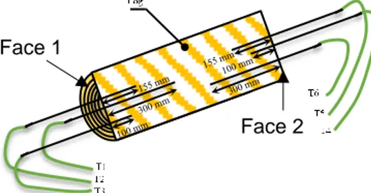
(3) bioresources.com. PEER-REVIEWED ARTICLE. production. The practice of additional holes for thermocouples would have been timeconsuming and resulted in waste of veneers.. Geometrical log measurement. Log intsrumentation. Heating log in boiler and data acquisition. Inverse identification method. Fig. 1. Measurement and model step flowchart. Sampling and Material Diffusivity ratio identification sample The thermal diffusivity ratio (𝜒) is the ratio of the thermal diffusivity in the radial direction (𝛼𝑟 ) to the thermal diffusivity in the longitudinal direction (𝛼𝑙 ). The log was soaked in a laboratory-scale boiler with a regulated temperature (± 1 °C). To assess the thermal changes that the log underwent during the 70 °C water-soaking process, the log temperature at three different radial positions and depths (longitudinally) of each log end face (Fig. 2) was measured using 5-mm diameter stainless steel sheath K-type thermocouples and an Agilent 34970A acquisition station (Agilent Technologies, Santa Clara, CA, USA) with an Agilent 34901A acquisition card (Agilent technologies, Santa Clara, CA, USA). The thermocouples were inserted in holes drilled using an extra-long (5 mm diameter and 400 mm long) drill bit (Dormer Pramet, Elgin, IL, USA). The data acquisition was set to record the temperature of the six logs and the surrounding water (another thermocouple was placed in the soaking bath) every minute until the whole log reached a homogeneous temperature after about 32 h (Fig. 2). To compute the longitudinal to radial thermal diffusivity ratio, one green Douglas fir log (CFBL, Ussel, France) with a diameter that ranged from 345 mm to 380 mm and a length of 680 mm was investigated. The log weighed 53.42 kg before soaking. Measurement with a balance (OHAUS I-20-W, Nänikon, Uster, Switzerland) indicated a green specific gravity of approximately 770 kg/m3, which was in accordance with the green specific gravity of 753 kg/m3 reported by Miles and Smith (2009). The log was 45 years old with a mean annual increment of 8.0 ± 0.5 mm. Face 1. Face 2. Fig. 2. An instrumented log with three thermocouples on one side and three thermocouples being inserted on the other face as described in Table 1. Based on the different radial and longitudinal locations of the thermocouples and a finite element model (FEM), the ratio was evaluated with an inverse identification method. The chosen thermocouples locations relied on the FEM model presented below, and they are listed in Table 1. Locations were chosen to maximize the temperature difference between each thermocouple and improve the accuracy of 𝜒 ratio determination. Two Frayssinhes et al. (2020). “Green wood diffusivity,”. BioResources 15(3), 6539-6549.. 6541.

(4) bioresources.com. PEER-REVIEWED ARTICLE. thermocouples (N°2 and N°5) were located opposite to each other to verify that temperature evolutions were similar on each log side. Table 1. Thermocouple Locations to Determine the Thermal Diffusivity Ratio (𝜒) Thermocouple N°. Depth (mm) 300 155 100 100 155 300. 1 2 3 4 5 6. End face 1. End face 2. Radius (mm) 0 50 100 0 50 100. Figure 3 presents the temperature kinetic for each thermocouple. Thermocouples 2 and 5, which were located at a depth of 155 mm and a radial position of 50 mm, exhibited a similar thermal evolution with a maximum gap of 0.8 °C. The first thermocouple located in the center had the slowest kinetics, which was expected. Additionally, the temperature recorded by the fourth thermocouple, which was located at the edge of the log, increased fastest. For example, after 7 h, the first thermocouple reached approximately 23 °C, and the third thermocouple reached approximately 51 °C. 70. Temperature (°C). 60 T water. 50. T1 d=300 r=0 40. T2 d=155 r=50. 30. T3 d=100 r=100 T4 d=100 r=0. 20. T5 d=155 r=50 10. T6 d=300 r=100. 0 0. 5. 10. 15. 20. 25. 30. 35. Time (h) Fig. 3. The temperature evolution recorded by the six thermocouples. Radial diffusivity identification sample Eighteen Douglas fir logs from five different trees with diameters ranging from 350 mm to 500 mm and lengths of 800 mm were heated at various temperatures from 55 °C to 80 °C in the same boiler. The tree identification numbers, the log numbers, and the log radii are summarized in Table 2. The diffusivity ratios of these logs were similar to those measured with the fully monitored log from the previous subsection. This simplification allowed the use of only one thermocouple for each log to identify both radial and longitudinal thermal diffusivities. This experimental setup, which involved only one thermocouple, was chosen due to its suitability for the use by manufacturers to check their own wood stock and optimize their soaking process times correspondingly. The geometric center of each log was drilled to insert a K-type thermocouple. The temperature was acquired each minute using the same data recorder as previously described.. Frayssinhes et al. (2020). “Green wood diffusivity,”. BioResources 15(3), 6539-6549.. 6542.

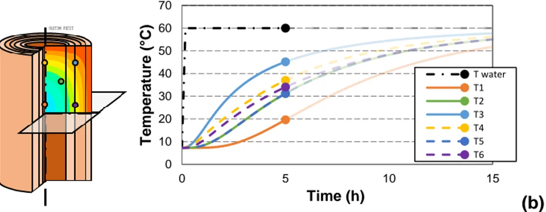
(5) bioresources.com. PEER-REVIEWED ARTICLE. Table 2. Log Characterization and Diffusivities Found by Both Inverse Methods (Analytical and FEM) Tree ID. Log N°. 0 0 1 1 1 1 2 2 2 2 2 3 3 3 4 4 4 4. 1 2 2 3 4 5 2 3 4 5 6 2 4 5 1 2 3 4. Tini Log Depth of Before Radius Measurement Soaking (mm) (mm) (°C) 210 435 12 200 435 11 260 370 13 245 370 11 235 370 11 230 370 11 255 370 14 250 370 14 250 370 13 240 370 13 240 370 16 190 370 19 175 370 22 165 370 22 235 370 20 225 370 20 230 370 19 220 370 21. Tmax Soaking Temp. (°C) 70 70 65 65 65 65 65 65 65 65 70 81 67 67 55 55 81 67. Diffusivity Analytical Method (mm².s-1) 0.215 0.175 0.179 0.163 0.157 0.16 0.184 0.174 0.189 0.179 0.182 0.187 0.146 0.156 0.146 0.155 0.192 0.155. Error 𝜀𝑟 Analytical Method (°C.h-1) 0.038 0.028 0.015 0.019 0.015 0.015 0.018 0.016 0.023 0.023 0.046 0.053 0.038 0.034 0.012 0.014 0.056 0.018. Diffusivity FEM Method (mm².s-1) 0.222 0.181 0.181 0.164 0.158 0.164 0.186 0.178 0.192 0.183 0.186 0.192 0.15 0.158 0.147 0.156 0.194 0.158. Error 𝜀𝑟 FEM Method (°C.h-1) 0.035 0.029 0.014 0.018 0.014 0.015 0.017 0.013 0.022 0.021 0.043 0.047 0.039 0.031 0.014 0.013 0.052 0.019. Methods to Determine the Temperature Evolution Knowing the Thermal Diffusivity of Wood First approach: FEM to determine the temperature at any location A finite element model was developed to determine the temperature evolution in the log. It was implemented in CAST3M (CEA Saclay 2018, Gif sur Yvette, France). The log was perfectly cylindrical (Fig. 4), so it was simplified to an axisymmetric geometry with the axisymmetry axis corresponding to the log pith. A second plane of symmetry, normal to the log axis, was considered at the middle length of the log. Both symmetries increased the speed of computation. The model was composed of a four node quadrangle (QUA4) with linear interpolation. The entry parameters were water temperature, initial log temperature, log radius, measuring locations, 𝜒 ratio, and wood radial diffusivity.. Temperature (°C). 70 60 50 40. T water T1 T2 T3 T4 T5 T6. 30 20 10 0 0. (a). 5. 10. Time (h). 15. (b). Fig. 4. (a) The finite element model and position of the measuring points used to determine (b) temperature evolution of the measuring points during soaking at 60 °C. 𝜒;. Frayssinhes et al. (2020). “Green wood diffusivity,”. 6543. BioResources 15(3), 6539-6549..

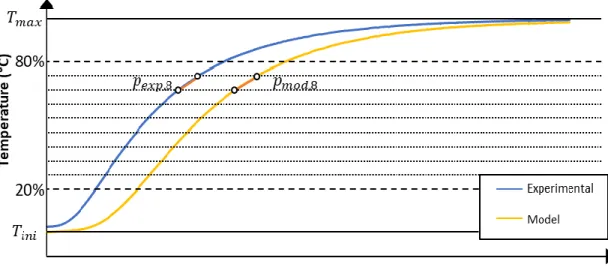
(6) bioresources.com. PEER-REVIEWED ARTICLE. Second approach: Analytic model to determine the temperature of log pith The mean temperature of the log center was determined by the heat propagation equation (Jannot and Moyne 2016) for the radial and longitudinal directions. Equations are derived from the first thermodynamic law for a perfect cylinder with a radius 𝑅 initially at the temperature 𝑇ini instantly immerged inside an infinite volume of fluid at a constant 𝑇max temperature (at t = 0, the log surface temperature is 𝑇max ). Accordingly, the temperature in the radial direction was calculated with Eq. 1, 𝑇(r,t) = 𝑇max +. 2(𝑇ini −𝑇max ) 𝑅. ∑𝑁 𝑛=1. 𝐽0 (𝜔n ∙𝑟) 𝜔n ∙𝐽1 (𝜔n. 2. e−𝑎r ∙𝜔𝑛∙𝑡 ∙𝑅). (1). where 𝑇max is the water soaking temperature (°C) inside the boiler, 𝑇ini is the initial log temperature (°C), 𝑅 is the log radius (mm), 𝐽0 and 𝐽1 are the Bessel functions; 𝜔n is the nth root of the Bessel equation 𝐽0 divided by the radius , 𝑎r is radial diffusivity (mm2.s-1), 𝑟 is the radial position (mm) of the measurement, and 𝑡 is the time (s). The temperature in the longitudinal direction was calculated with Eq. 2, 𝑇(x,t) = 𝑇max +. 4(𝑇ini −𝑇max ) π. 1 ∑∞ 𝑛=1 2𝑛+1 sin ((2𝑛. + 1). 𝜋∙𝑥 𝐿. )∙e. −(2𝑛+1)2. π2 ∙𝑎l ∙𝑡 L2. (2). where 𝑥 the radial position (mm) of the measurement, 𝛼l is the longitudinal global thermal diffusivity (mm2.s-1), and 𝐿 is the log length (mm). Accordingly, the temperature in the log center is a combination of these two temperatures calculated using the Von Neumann formulation (Eq. 3): [. 𝑇(x,r,t) −𝑇max 𝑇ini −𝑇max. 𝑇(x,t) −𝑇max. ] = [𝑇. ini −𝑇max. 𝑇(r,t) −𝑇max. ]×[𝑇. ini −𝑇max. ]. (3). This analytical method was computed with Python libraries to determine the log temperature as a function of the water temperature surrounding the log in the boiler, the initial log temperature, the log radius, the measurement position, and the radial and longitudinal wood thermal diffusivities. Thermal Diffusivity Determination by Inverse Identification The ratio (𝜒) and the radial diffusivity (𝛼) were optimized to minimize the mean of Δ𝑇 the root mean square error (RMSE) between the slope ( Δ𝑡 ) of the model and the slope of the experimental data. This method was chosen to avoid a time shift due to the thermal transition effect at the beginning of the measurement. The experimental and model curves did not need to be synchronized in this case, as the error was relative to a differential temperature and a differential time. The RMSE was calculated by splitting each curve into nine equal parts from 20% to 80% of the thermal variation (Δ𝑇 = 𝑇max – Tini ). Figure 5 presents two temperature evolution curves, the first of which is the experimental curve. The second curve is a non-optimized model, which explains the notable gap between the two curves. Segments in Fig. 5 represent the evolution of the temperature of the eighth part. The root mean square error of the slopes was calculated using Eq. 4 for the nine considered parts, √∑. 𝜀r (𝛼, 𝜒) =. 9 i=1. (𝑝exp,i −𝑝mod,i ). 2. (4). 9. Frayssinhes et al. (2020). “Green wood diffusivity,”. BioResources 15(3), 6539-6549.. 6544.

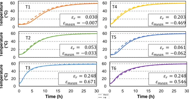
(7) bioresources.com. PEER-REVIEWED ARTICLE. where 𝑝exp,i is the slope of the ith part of the experimental elevation curve, 𝑝mod,i is the slope of the ith part of the modeling elevation curve, and 𝜀r is the error that must be minimized for each measured temperature.. Fig. 5. The optimization method used to find the lowest slope difference. In addition, the mean error 𝜀mean was computed, which indicates if the model underestimates or overestimates the temperature depending on the sign of the mean error; it was calculated for each thermocouple curve with Eq. 5: 𝜀mean (𝛼, 𝜒) =. ∑9𝑖=1(𝑝exp,i –𝑝mod,i ). (5). 9. To determine 𝜒, the mean of the root mean square error (𝜀r ) was minimized using Eq. 6, 𝜀̅r (𝛼, 𝜒) = min (. ∑6𝑖=1 𝜀r,j 6. ). (6). where 𝜀r,j is the root mean square error of the jth thermocouple of the log. These minimization methods were employed to reach the best agreement between the experimental data and the model for all of the thermocouples globally.. RESULTS AND DISCUSSION Ratio and Radial Diffusivity Identification on One Log To determine the ratio of the longitudinal diffusivity to radial diffusivity, an FEM model was established with five nodes located in the thermocouple position because T2 and T5 were located in parallel positions on different sides of the log. This model was run for a diffusivity ratio ranging from 1 to 7 with steps of 0.1 and a radial thermal diffusivity ranging from 0.1 mm2.s-1 to 0.3 mm2.s-1 with steps of 0.003 mm2.s-1. A total of 2,700 simulations were performed to find the best combination of the radial diffusivity and diffusivity ratio by minimizing the error (𝜀r ). Figure 6 presents an example of temperature evolution with the results of the optimized FEM model for the experimental data obtained. Frayssinhes et al. (2020). “Green wood diffusivity,”. BioResources 15(3), 6539-6549.. 6545.

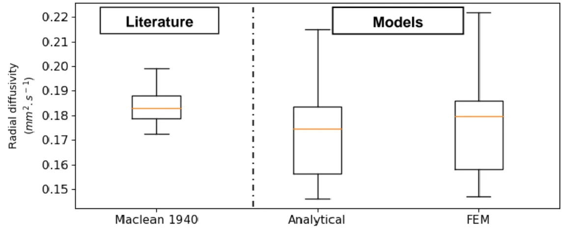
(8) bioresources.com. PEER-REVIEWED ARTICLE. Temperature (°C). 60. Temperature (°C). 60. Temperature (°C). during Douglas fir log soaking at 60 °C. A thermal radial diffusivity value equal to 0.208 mm2.s-1 and a thermal diffusivity ratio of 2.4 were observed. The identified ratio value was comparable to those in the literature, which ranged from 2 to 2.5 for softwood (MacLean 1940; Kollmann 1951; Maku 1954; Perré and Turner 2001). 60. T1. 40. T4. 40. 𝜀𝑟 = 0.030 𝜀𝑚𝑒𝑎𝑛 = −0.007. 20 0. 𝜀𝑟 = 0.203 𝜀𝑚𝑒𝑎𝑛 = −0.469. 20 0 60. T2. 40. 𝜀𝑟 = 0.053 𝜀𝑚𝑒𝑎𝑛 = −0.033. 20 0 60. 0. T6. 40. 𝜀𝑟 = 0.248 𝜀𝑚𝑒𝑎𝑛 = 0.671. 20. 0 0. 𝜀𝑟 = 0.061 𝜀𝑚𝑒𝑎𝑛 = −0.062. 20. 60. T3. 40. T5. 40. 5. 10. 15. 20. 25. 30. Time (h). 𝜀𝑟 = 0.248 𝜀𝑚𝑒𝑎𝑛 = 0.546. 20. 0 0. 5. 10. 15. 20. 25. 30. Time (h). Fig. 6. The experimental temperature evolutions versus the FEM model. The slope of the temperature kinetic was similar to that of the experimental data, which illustrated the robustness of the approach, even though it was based upon several assumptions (homogeneous wood within the volume, cylindrical shape, and constant thermal diffusivity regardless of temperature). The error (𝜀mean ) was negative for the thermocouples near the log pith (0 mm and 50 mm from the center), which indicated that the model for those positions overestimated the temperature. In addition, the positive 𝜀mean value for the thermocouples at 100 mm from the center indicated an underestimation of the temperature. Moreover, the difference in moisture content between sapwood and heartwood in Douglas-fir (Mothe et al. 2000) affects the thermal diffusivity locally and the accuracy of the global identification. Radial diffusivity identification on 18 logs A review of the literature found that only MacLean (1940) gives values of thermal diffusivity for green Douglas fir with a moisture content ranging from 22.6% to 31.3% in heated water. This author gives only seven values, which is not enough to highlight material dispersion. MacLean’s (1940) radial diffusivity data are shown in Fig. 7 for reference alongside the radial thermal diffusivity data obtained on the 18 logs examined in this study. The inverse identification method was used for the 18 green Douglas fir logs with a fixed ratio (𝜒) of 2.4 according to the previous calculation. The radial thermal diffusivities computed with both the FEM and the analytical methods are presented in Table 2. The radial diffusivity determined by the analytical method exhibited an approximately 10% higher scattering and a higher error than the radial diffusivity determined by FEM. Figure 8 contains the correlation matrix between the different variables considered in this study, Frayssinhes et al. (2020). “Green wood diffusivity,”. BioResources 15(3), 6539-6549.. 6546.

(9) bioresources.com. PEER-REVIEWED ARTICLE. including where the logs were extracted from, log radius, initial temperature (Tini), water temperature (Tmax) during soaking, both radial diffusivities from the analytical and finite element methods, and their respective errors. Literature. Models. Fig. 7. A comparison of the models results and the values reported by MacLean (1940). Tree ID. Log radius. Tini. Tmax. Diffusivity Error Diffusivity analytical analytical FEM method method method. Error FEM method. Fig. 8. Correlation matrix between the different variables. A high correlation coefficient was observed between the errors and the temperature; this may have been due to the evolution of the thermal diffusivity value within the temperature. However, the two methods (analytical and FEM) found similar radial thermal diffusivity values with a correlation coefficient of 1.0, which showed the high accuracy of both approaches. Application Example A typical application for an industrial is to estimate the time to heat a log from an initial temperature at 20 °C to 50 °C in boiler. In hypothesis, this log has a diameter of Frayssinhes et al. (2020). “Green wood diffusivity,”. BioResources 15(3), 6539-6549.. 6547.

(10) PEER-REVIEWED ARTICLE. bioresources.com. 500 mm and a length of 2700 mm. With such settings, the time to reach 95% of the 50 °C target is about 50 h for a 2.4 ratio between the radial and longitudinal thermal diffusivities, and a radial thermal diffusivity of 0.175 mm2.s-1.. CONCLUSIONS 1. An analytical model and an FEM model were created to identify the temperature evolution inside the log during soaking prior to processing by rotary peeling. These models considered the wood radial thermal diffusivity and the diffusivity ratio of longitudinal to radial diffusivity, which were both homogeneous within the log volume. In addition, the log geometry was perfectly cylindrical. 2. A soaking monitoring system was developed to measure the temperature inside Douglas fir logs directly inside the boiler. The experimental temperature evolution inside the log was compared with the diffusivity model optimized via the inverse identification method to assess the global radial thermal diffusivity of the log. The values obtained in this study were comparable to those from the literature for green Douglas fir wood. A thermal diffusivity ratio of 2.4 and a mean radial diffusivity of 0.171 mm2.s-1 were calculated with the analytical method, and a mean radial diffusivity of 0.175 mm2.s-1 was calculated with the FEM model. 3. This method can be used easily and at a low cost by the peeling industry when peeling a new species to ensure the best time/temperature ratio for the soaking pretreatment of the subsequent peeling process.. ACKNOWLEDGMENTS This work was financially supported by Burgundy Regional Council and the French Ministry of Agriculture and Forestry.. REFERENCES CITED Aydin, I., Colakoglu, G., and Hiziroglu, S. (2006). “Surface characteristics of spruce veneers and shear strength of plywood as a function of log temperature in peeling process,” International Journal of Solids and Structures, 43(20), 6140–6147. DOI: 10.1016/j.ijsolstr.2005.05.034 Corder, S. E., and Atherton, G. H. (1963). Effect of peeling temperatures on Douglas fir veneer, Corvallis, Or.: Forest Research Laboratory, Oregon State University. Dupleix, A., Denaud, L., Bleron, L., Marchal, R., and Hughes, M. (2013). “The effect of log heating temperature on the peeling process and veneer quality: beech, birch, douglas-fir and spruce case studies,” European journal of Wood and Wood Products, 71(2), 163-171. DOI: 10.1007/s00107-012-0656-1 Dupleix, A., Kusiak, A., Hughes, M., and Rossi, F. (2012). “Measuring the thermal properties of green wood by the transient plane source (TPS) technique,” Holzforschung 67(4), 437-445. DOI: 10.1515/hf-2012-0125. Frayssinhes et al. (2020). “Green wood diffusivity,”. BioResources 15(3), 6539-6549.. 6548.

(11) PEER-REVIEWED ARTICLE. bioresources.com. Frayssinhes, R., Stefanowski, S., Denaud, L., Girardon, S., Marcon, B., and Collet, R. (2019). “Peeled veneer from Douglas-fir: Soaking temperature influence on the surface roughness,” in: Proceedings of the 24th International Wood Machining Seminar, Corvallis, OR, USA, pp. 237-245. Gustafsson, S. E. (1991). “Transient plane source techniques for thermal conductivity and thermal diffusivity measurements of solid materials,” Review of Scientific Instruments, 62(3), 797-804. DOI: 10.1063/1.1142087 Hecker, M. (1995). “Peeled veneer from Douglas-fir - Influence of round wood storage, cooking, and peeling temperature on surface roughness,” in: Proceedings of the 12th International Wood Machining Seminar, Kyoto. Jannot, Y., and Moyne, C. (2016). Transferts Thermiques: Cours et 55 Exercices Corrigés. Kollmann, F. (1951). Technologic des Holzes und der Holzwerkstoffe. . Bd. 1. MacLean, J. D. (1940). “Relation of wood density to rate of temperature change in wood in different heat medium,” Proceeding of American Wood Preserver’s Association, 220-248. Maku, T. (1954). “Studies on the heat conduction in wood: The present study is a discussion on the results of investigations made hitherto by author on heat conduction in wood.” Miles, P. D., and Smith, W. B. (2009). Specific Gravity and other Properties of Wood and Bark for 156 Tree Species Found in North America, U.S. Department of Agriculture, Forest Service, Northern Research Station, Newtown Square, PA, USA. DOI: 10.2737/NRS-RN-38 Mothe, F., Marchal, R., and Tatischeff, W. T. (2000). “Sécheresse à coeur du Douglas et aptitude au déroulage: Recherche de procédés alternatifs d’étuvage. I. Répartition de l’eau dans le bois vert et réhumidification sous autoclave,” Annals of Forest Science 57(3), 219-228. Parker, W. J., Jenkins, R. J., Butler, C. P., and Abbott, G. L. (1961). “Flash method of determining thermal diffusivity, heat capacity, and thermal conductivity,” Journal of Applied Physics 32(9), 1679-1684. DOI: 10.1063/1.1728417 Perré, P., and Turner, I. (2001). “Determination of the material property variations across the growth ring of softwood for use in a heterogeneous drying model. Part 2. Use of homogenisation to predict bound liquid diffusivity and thermal conductivity,” Holzforschung 55(4). DOI: 10.1515/HF.2001.069 Rohumaa, A., Antikainen, T., Hunt, C. G., Frihart, C. R., and Hughes, M. (2016). “The influence of log soaking temperature on surface quality and integrity performance of birch (Betula pendula) veneer,” Wood Science and Technology 50(3), 463-474. DOI: 10.1007/s00226-016-0805-5 Sonderegger, W., Hering, S., and Niemz, P. (2011). “Thermal behaviour of Norway spruce and European beech in and between the principal anatomical directions,” Holzforschung 65(3). DOI: 10.1515/hf.2011.036 Thibaut, B. (1988). “Le processus de coupe du bois par déroulage,” Atelier duplication [U.S.T.L.]. Article submitted: March 17, 2020; Peer review completed: June 13, 2020; Revised version received and accepted: July 1, 2020; Published: July 8, 2020. DOI: 10.15376/biores.15.3.6539-6549. Frayssinhes et al. (2020). “Green wood diffusivity,”. BioResources 15(3), 6539-6549.. 6549.

(12)