Combining local regularity estimation and total variation optimization for scale-free texture segmentation

To link to this article : DOI :

10.1109/TCI.2016.2594139

URL :

http://dx.doi.org/10.1109/TCI.2016.2594139

To cite this version :

Pustelnik, Nelly and Wendt, Herwig and Abry,

Patrice and Dobigeon, Nicolas Combining local regularity estimation and

total variation optimization for scale-free texture segmentation. (2016)

IEEE Transactions on Computational Imaging, vol. 2 (n° 4). pp. 468-479.

ISSN 2333-9403

O

pen

A

rchive

T

OULOUSE

A

rchive

O

uverte (

OATAO

)

OATAO is an open access repository that collects the work of Toulouse researchers and

makes it freely available over the web where possible.

This is an author-deposited version published in :

http://oatao.univ-toulouse.fr/

Eprints ID : 17138

Any correspondence concerning this service should be sent to the repository

administrator:

staff-oatao@listes-diff.inp-toulouse.fr

Combining Local Regularity Estimation and Total

Variation Optimization for Scale-Free

Texture Segmentation

Nelly Pustelnik, Member, IEEE, Herwig Wendt, Member, IEEE, Patrice Abry, Fellow, IEEE,

and Nicolas Dobigeon, Senior Member, IEEE

Abstract—Texture segmentation constitutes a standard image

processing task, crucial for many applications. The present contri-bution focuses on the particular subset of scale-free textures and its originality resides in the combination of three key ingredients: First, texture characterization relies on the concept of local regu-larity; Second, estimation of local regularity is based on new multi-scale quantities referred to as wavelet leaders; Third, segmentation from local regularity faces a fundamental bias variance tradeoff. In nature, local regularity estimation shows high variability that impairs the detection of changes, while a posteriori smoothing of regularity estimates precludes from locating correctly changes. In-stead, the present contribution proposes several variational prob-lem formulations based on total variation and proximal resolutions that effectively circumvent this tradeoff. Estimation and segmenta-tion performance for the proposed procedures are quantified and compared on synthetic as well as on real-world textures.

Index Terms—Convex functions, image texture analysis,

opti-mization methods, wavelet transforms.

I. INTRODUCTION

A. Fractal Based Texture Characterization

T

EXTURE characterization and segmentation are long-standing problems in Image Processing that received sig-nificant research efforts in the past and still attract considerable attention. In essence, texture consists of a perceptual attribute. It has thus no unique formal definition and has been envisaged using several different mathematical models, mostly relying on the definition and classification of either geometrical or statis-tical features, or primitives (cf., e.g., [1], [2] and references therein for reviews). Texture analysis can be performed us-ing either parametric models (ARMA [3], Markov [4], Wold [5]) or non parametric approaches (e.g., time-frequency and Gabor distributions [6], [7]). Amongst this later class, multiscale representations (wavelets, contourlet, ...) have repeatedly been reported as central in the last two decades (cf., e.g., [8]–[11]).

Manuscript received February 17, 2016; revised June 22, 2016 and July 12, 2016; accepted July 20, 2016. Date of publication July 27, 2016; date of current version November 4, 2016. This work was supported by the CNRS GdR ISIS junior research project GALILEO and ANR under Grants AMATIS #112432. The associate editor coordinating the review of this manuscript and approving it for publication was Prof. Jong Chul Ye.

N. Pustelnik and P. Abry are with the Laboratoire de Physique, University of Lyon, ENS de Lyon, CNRS, Lyon F-69342, France (e-mail: nelly.pustelnik@ ens-lyon.fr; patrice.abry@ens-lyon.fr).

H. Wendt and N. Dobigeon are with the IRIT at INP-ENSEEIHT, University of Toulouse and CNRS, Toulouse 31071, France (e-mail: herwig.wendt@irit.fr; nicolas.dobigeon@enseeiht.fr).

Color versions of one or more of the figures in this letter are available online at http://ieeexplore.ieee.org.

Digital Object Identifier 10.1109/TCI.2016.2594139

They notably showed significant relevance for the large class of scale-free textures, often well accounted for by the celebrated fractional Brownian motion (fBm) model, on which the present contribution focuses. Examples of such textures are illustrated in Fig. 1(a). While scale free-like texture segmentation has been mainly conducted by exploiting the statistical distribution of the pixel amplitudes [12]–[14], the present paper investigates the relevance of local regularity-based analysis.

Deeply tied to multiscale analysis, the fractal and multifractal paradigms [15], [16] have been intensively used for scale-free texture characterization (cf., e.g., [17], [18]). Scale-free textures are essentially measured jointly at several scales, or resolutions. From the evolution across scales of such multiscale measures, semi-parametrically modeled as power-laws and thus insensi-tive to texture resolution, scaling exponents are then extracted and used as characterizing features. Such fractal features have been extensively used for texture characterization, notably for biomedical diagnosis (e.g., [19]–[22]), satellite imagery [23] or art investigations [24], [25].

Often, in applications, it is assumed a priori that fractal prop-erties are homogenous across the entire piece of texture to char-acterize, thus permitting reliable estimates of the fractal features (scaling exponents). However, in numerous situations, images actually consist of several pieces, each with different textures, and hence different fractal properties. Analysis becomes thus far more complicated as it requires to segment the texture into pieces (with unknown boundaries to be estimated) within which fractal properties can be considered homogeneous (i.e., fractal attributes are constant), yet unknown.

B. Local Regularity and H¨older Exponent

To address such situations, the present contribution elabo-rates on the fractal paradigm, by a local formulation relying on the notion of pointwise regularity. The local regularity of a function (or sample path of a random field) at a given location x∈ R2 _{is most commonly quantified by the H¨older exponent}

h(x) [26]. It is defined as the scaling exponent extracted from the a priori assumed power law dependence of the coefficients of a multiscale representation X(a, x) (e.g., the modulus of wavelet coefficients [11]), across the scales a, in the limit of fine scales: X(a, x) ≃ η(x)ah(x) _{when a→ 0. Theoretically,}

the collection of H¨older exponents h(x) for all x ∈ R2 _yields

access to the multifractal properties (and spectrum) of the tex-ture, and thus consists of a multiscale higher-order statistics feature characterizing the texture [26], [27].

Wavelet coefficients are the most popular multiscale represen-tation used to perform fractal analysis. Yet, it has recently been shown that, in the context of multifractal analysis and thus of local regularity estimation, wavelet coefficients are significantly outperformed by wavelet leaders, consisting of local suprema of wavelet coefficients [26]–[29]. While the methods proposed in the present contribution could be used with any multiscale representation, reported and discussed results are thus explicitly obtained using wavelet leaders.

For each location x, h(x) is classically estimated via a linear regression inlog X(a, x) versus log a coordinates and is thus naturally framed into a classical bias-variance trade-off: Point-wise estimates (relying only on the X(a, x) at sole location x) show very large variances. Conversely, averaging in space-windows either the X(a, x) or directly the estimates of h(x) results in significant bias. In either case, the reliable and accurate detection and localization of actual changes in h is precluded. This explains why local regularity remains so far barely used for signal or texture characterization and segmentation (see, a contrario, [29]–[33]).

C. Goals, Contributions and Outline

In the present contribution, elaborating on preliminary at-tempts [29], [32], the overall goal is to enable the actual use of local regularity for performing the segmentation of scale-free textures into areas with piece-wise constant fractal character-ization. This strategy has the great advantage of being fully nonparametric, since it does not require any explicit (statistical) modeling of the textures to be segmented. To that end, it aims to marry wavelet-leader based estimation of local regularity (with no a priori smoothing) to segmentation procedures formulated as variational problems and constructed on total variation (TV) op-timization procedures and proximal based resolutions. Wavelet-leader based estimation of H¨older exponents (as defined and detailed in Section II) is first applied locally throughout the en-tire image. Then, to go beyond a naive a posteriori smoothing and threshold-based segmentation procedure (as described in Section III-A), three different TV-based segmentation proce-dures are theoretically devised: 1) Local estimates of h are sub-jected a posteriori to a TV based denoising procedure, followed by a thresholding step for segmentation (cf., Section III-B); 2) Local estimation of h is a priori embodied into the TV based procedure aiming to favor piecewise constant estimates, thresholding for segmentation is performed a posteriori (cf., Section III-C); 3) Local estimates of h are subjected a posteriori to a TV based segmentation procedure, avoiding the denois-ing/thresholding steps (cf., Section III-D). This later procedure is inspired by the convex relaxation of the Potts model detailed in [34], [35].

In Section IV, the performance of the proposed TV segmen-tation procedures are compared and discussed for samples of synthetic textures with piece-wise constant h, obtained from a multifractional model, whose definition is customized by our-selves to achieve realistic textures (described in Section II-D). Several different geometries and different sets of values for the regularity h of the different segments are considered. Further-more, the impact of the TV-regularization parameter is

investi-gated. These procedures are also compared against two texture segmentation procedures chosen because they are considered state-of-the art in the dedicated literature [7], [36]. The pro-posed approaches are further shown at work on samples chosen within well accepted references texture databases, such as the Berkeley Segmentation Dataset. Synthesis and analysis proce-dures will be made publicly available at the time of publication. Note that the present contribution significantly differs from the preliminary works [29], [32] in that several methods involving TV are designed, and these methods are unified and compared on synthetic images and real-world textures.

II. H ¨OLDEREXPONENT ANDWAVELETLEADERS

A. H¨older Exponent and Local Regularity: Theory

Let f =¡f(x)¢_x∈Ω with x= (x1, x2) denote the bounded

2D function (image) to analyze. The local regularity around location x0 is quantified using the so-called H¨older exponent

h(x0), formally defined as the largest α > 0, such that there exist

a constant χ >0 and a polynomial Px0 of degree lower than α,

such thatkf (x) − Px0(x)k ≤ χkx − x0k

α_{in a neighborhood x}

of x0, wherek · k denotes the Euclidean norm [26]. When h(x0)

is close to0, the image is locally highly irregular and close to discontinuous. Conversely, large values of h(x0) correspond to

locations where the field is locally smooth. An example of a texture with piece-wise constant function h(x) is illustrated in Fig. 1(a).

Though the theoretical definition of the H¨older exponent above can be used for the mathematical study of the regularity properties of fields, it is also well-known that it turns extremely uneasy for practical purposes and for the actual computation of h from real world data. Instead, multiscale representations pro-vide natural alternate ways for the practical quantification of h [23], [27], [28], [30]. It is however nowadays well documented that the sole wavelet coefficients do not permit to accurately estimate local regularity [26], [27]. Early contributions on the subject proposed to relate local regularity to the skeleton of the continuous wavelet transform [11], [23], which however does not permit to achieve estimation of h at each location x as tar-geted here. Instead, it has been recently shown that an efficient estimation of h can be conducted using wavelet leaders [26], [27]. They are defined as local suprema of the coefficients of the discrete wavelet transform (DWT) and thus inherit their computational efficiency.

B. H¨older Exponent and Wavelet Leaders

1) Wavelet Coefficients: Let φ and ψ denote respectively the scaling function and mother wavelet, defining a 1D multiresolu-tion analysis [11]. The mother wavelet ψ is further characterized by an integer Nψ ≥ 1, referred to as the number of vanishing

mo-mentsand defined as:∀k = 0, 1, . . . , Nψ − 1,

R

|t|k_{ψ(t)dt ≡ 0}

and R |t|Nψ_{ψ(t)dt 6= 0. From these univariate functions, 2D}

wavelets are defined as (

ψ(0)(x) = φ(x1)φ(x2), ψ(1)(x) = ψ(x1)φ(x2),

ψ(2)(x) = φ(x1)ψ(x2), ψ(3)(x) = ψ(x1)ψ(x2).

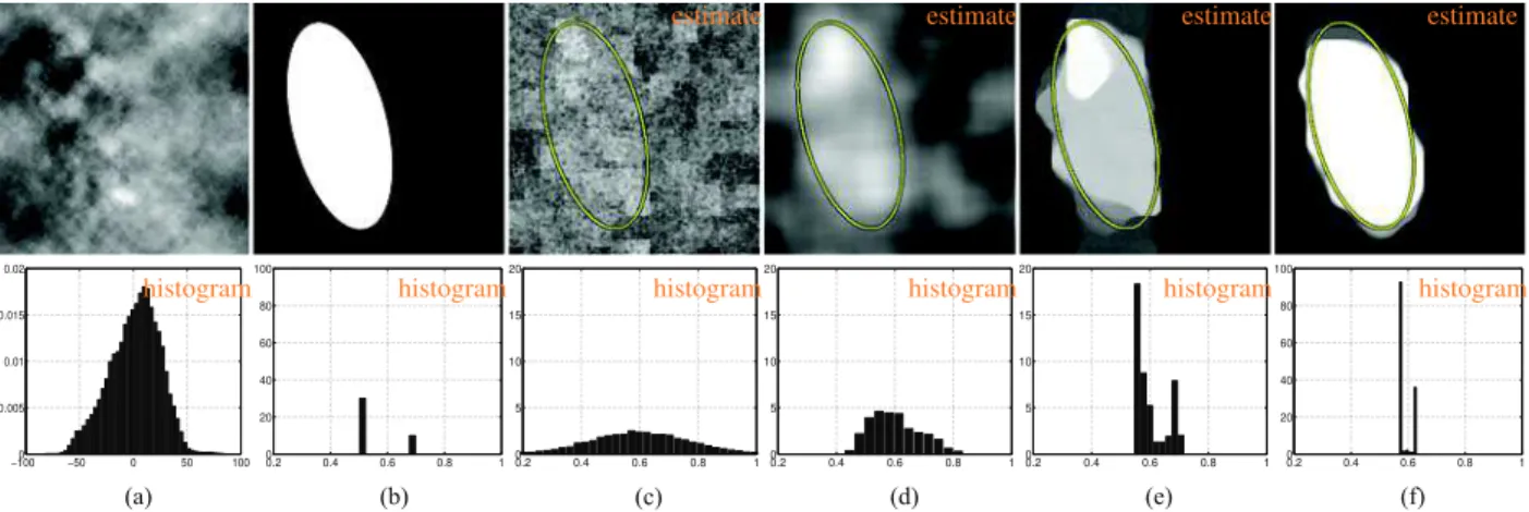
Fig. 1. Illustration of the local regularity estimation from a multifractional data. Top row: (a) image f ; (b) the original local regularity h from which f is generated, the area in black (resp. white) corresponds to a local regularity of0.5 (resp. 0.7); (c) an estimation based on wavelet leaders; (d) smooth estimate ofbh described in Section III-A; (e) estimation using the method described in Section III-B; (f) estimation based on the method described in Section III-C. Bottom row: histograms corresponding to top row.

The 2D-DWT (L1-normalized) coefficients of the image f are defined as

Y_f(m )(j, k) = 2−jDf, ψ_j,k(m )E (2) where {ψ_j,k(m )(x) = 2−j_ψ(m )₍₂−j_{x− k), j ∈ N}∗_{, k∈ N}2_,

m= 0, 1, 2, 3} is the collection of dilated (to scales a = 2j₎

and translated (to locations x= 2j_{k, k= (k}

1, k2)) templates

of ψ(m )(x). Interested readers may refer to [11] for further details.

2) Wavelet Leaders: The wavelet leader Lf(j, k), at scale

2j _{and location x= 2}j_{k, is defined as the local supremum of}

all wavelet coefficients Y_f(m )(j′, k′) taken across all finer scales 2j′

≤ 2j_{, within a spatial neighborhood [26]–[28]}

L(γ )_f (j, k) = sup m={1,2,3} λ j ′ , k ′⊂3λj , k |2j γ_Y(m ) f (j ′_{, k}′_{)| (3)} where ₍ λ_{j,k = [k2}j_{,(k + 1)2}j₎ 3λj,k =S_{p∈{−1,0,1}}2λj,k+p. (4) The additional positive real parameter γ can be tuned to ensure minimal regularity conditions for the case where the image f to analyze can not be modeled as a strictly bounded 2D-function. It is set to γ= 1 for the present contribution and not further discussed. Interested readers are referred to [27], [28] for the details on the role and impact of parameter γ.

It has been proven in [26] that the H¨older exponent h(x) at location x is measured by wavelet leaders as

L(γ )_f (j, k) ≃ η(x)2j(h(x)+γ ) when 2j _{→ 0 (5)}

for x∈ λj,k, provided that Nψ is strictly larger than h(x).

Note that (5) implies that h can be estimated by linear re-gressions as the slope oflog2L

(γ )

f versus j, cf., (6)–(9) below

(similarly,log η could be obtained as the intercept, yet does not bear any information on local regularity and will hence not be further considered here).

C. H¨older Exponent Estimation

In the present contribution, the estimation of the H¨older ex-ponent is only performed using wavelet leaders L(γ )_f (j, k), as preliminary contributions [27]–[29], [32] report that wavelet leader based estimation outperforms those based on other mul-tiresolution quantities. To indicate that the estimation of h and the segmentation procedures proposed in Section III below could be applied using any other multiresolution quantity, e.g., the modulus of the 2D-DWT coefficients, a generic notation X(j, k) is used instead of the specific L(γ )_f (j, k). Yet, all nu-merical results in Section IV are obtained with wavelet leaders, X(j, k) = L(γ )_f (j, k).

In the discrete setting, H¨older exponents are estimated for the locations x= 2k associated with the finest scale j = 1, and we make use of the notation · when we are dealing with matrices, rather than with matrix elements, e.g.,

h=³h(k)´

k∈K,K = {1, . . . , N1} × {1, . . . , N2}.

As a preparatory step, the multiresolution quantity X is up-sampled in order to obtain as many coefficients at scales j >1 as at the finest scale j= 1

e

X(j, (k1, k2)) = X(j, (⌈2−jk1⌉, ⌈2−jk2⌉)) (6)

with 1 ≤ k1 ≤ N1, 1 ≤ k2≤ N2. With a slight abuse of

notation, we will continue writing X for the upsampled multiresolution coefficients ˜X.

The relation (5) can obviously be rewritten as

log2X(j, k) ≃ jh(k) + log2η(k) (7)

which naturally leads to the use of (weighted) linear regressions across scales for the estimation of h(x)

bh(k) =X

j

w(j, k) log2X(j, k). (8)

Combining (7) and (8) above shows that, for each location k, the weights w(j, k) must satisfy the following constraints to ensure

unbiased estimation [37] X j w(j, k) = 0 and X j jw(j, k) = 1. (9) Though unusual, let us note that the weights w(j, k) can in prin-ciple depend on location k. This will be used in the segmentation procedure defined in Section III-C. An illustration of such unbi-ased estimates, with a priori chosen w(j, k) that do not depend on location k, is presented in Fig. 1(c).

D. Piece-Wise Constant Local Regularity Synthetic Processes To illustrate the behavior of the segmentation procedures pro-posed in Section III as well as to quantify and compare seg-mentation performances from the different procedures, use is made of realizations of synthetic random fields with known and controlled piece-wise constant local regularity. These are con-structed as 2D multifractional Brownian fields [38], which are among the most widely used models for mildly evolving local regularity. Their definition has been slightly modified here to ensure the realistic requirement of homogeneous local variance across the entire image

f(x) = C(x) Z Ω eıxξ−1 |ξ|h(x)+1 2 dW(ξ) (10)

where dW(ξ) is 2D Gaussian white noise and h(x) denotes the prescribed H¨older exponent function. The normalizing factor C(x) ensures that the local variance of f does not depend on the location x. The details of the models do not matter much for the present work, as we are only targeting the control of local regularity of the field f(x). In the present contribution, the function h(x) is chosen as piece-wise constant. Numerical procedures permitting the actual synthesis of such fields have been designed by ourselves. A typical sample field of such a process is shown in Fig. 1(a).

III. LOCALREGULARITYBASEDIMAGESEGMENTATION

In this section, we will detail the proposed procedures for segmentation in homogeneous pieces of textures with constant local regularity.

A. Local Smoothing

A straightforward attempt for obtaining labels consists in thresholding the histogram of pointwise estimates obtained with (8) and (9). However, such a solution yields estimates with prohibitively large variance. This prevents the identification of modes in the histogram that would correspond to the different zones of constant local regularity, see Fig. 1(c) for an illustration. The variance can be reduced a posteriori by a local spatial smoothingwith a convolution filter g:

b

hS= g ∗ bh

where bh denotes the estimate described in Section II-C. For instance, g can model a local spatial average. In this work, we will consider a Gaussian smoothing parametrized by its standard deviation σ. Note that particular cases of this smoothing can be

expressed as a variational formulation bhS= arg min h∈RN 1 ×N 2    X k∈K   j2 X j=j1 w(j, k) log2X(j, k) − h(k)   2 + λkΓhk2F    (11)

wherek · kF denotes the Frobenius norm and the transformΓ

and the regularization parameter λ >0 are related to the convo-lution kernel g. In particular, when λ= 0, the smoothed solution b

hSreduces to its non-smoothed counterpart bh. An example of such an estimate with σ= 10 is given in Fig. 1(d). Clearly, the variance of bhS is smaller than the variance of bh (see Fig. 1(c) and (d)). Yet, it remains hard to identify separate modes in the histogram. What is more, the local averaging introduces bias at the edges of areas with constant h values, hence prevents any accurate localization of the regularity changes in the image. B. TV Denoising

To overcome these difficulties, we propose the use of TV based optimization procedures, naturally favoring sharp edges, instead of local spatial averages. It is well known that the bounded TV space, that is the space of functions with bounded ℓ1-norm of the gradient, allows to remove undesirable

oscilla-tions while it preserves sharp features. Rudin et al. [39] formal-ize this recovery problem as a variational approach involving a non-smooth functional referred to as TV. This has been widely used in image processing for image quality enhancement [39], [40] although it has been noted that it is not always well suited for restoration purposes due to the piece-wise constant nature of the restored images. In the present context of detection of local regularity changes, precisely such a piece-wise constant behavior of the solution is desired.

The corresponding minimization problem reads bhTV= arg min h∈RN 1 ×N 2    1 2 X k∈K   j2 X j=j1 w(j, k) log2X(j, k) − h(k)   2 +λTV(h)    (12) where TV(h) = N_X1−1 k1=1 N_X2−1 k2=1 q¡ (D1h)(k1, k2) ¢2 +¡(D2h)(k1, k2) ¢2 (D1h)(k1, k2) = h(k1+ 1, k2+ 1) − h(k1+ 1, k2) (D2h)(k1, k2) = h(k1+ 1, k2+ 1) − h(k1, k2+ 1).

The weights are a priori fixed, are independent of k, w(j, k) = w(j), and satisfy the constraints (9). Here, λ > 0 models the regularization parameter that tunes the piece-wise constant behavior of the solution. Several techniques have been proposed in the literature to solve (12), see for instance [40],

[41]. A forward-backward algorithm [42] applied on the dual formulation of (12) is used here.

An example of bhTV is displayed in Fig. 1(e) for λ= 6. It is piecewise constant and provides a satisfactory estimate of the true regularity displayed in Fig. 1(b). Furthermore, the his-togram of the estimates bhTV is pronouncedly peaked. Thresh-olding hence enables labeling for a preset number Q of classes. C. Joint Estimation of Regression Weights and Local

Regularity

The solution bhTVdescribed in the previous section is a two-step procedure that addresses the bias-variance trade-off diffi-culty by: (i) computing unbiased estimates of the H¨older expo-nents bh from X using (8) with fixed pre-defined weights w, and (ii) extracting areas with constant H¨older exponent based on these estimates bh using a variational procedure relying on TV. In this section, we propose a one-step procedure that directly yields piece-wise constant local regularity estimates bh from the multiresolution quantities X. The originality of this approach resides, on one hand, in the use of a criterion that involves di-rectly X, instead of the intermediary local estimates bh, and a TV-regularization; on other hand, in the fact that the weights w are jointly and simultaneously estimated instead of being fixed a priori. To this end, the weights w are subjected to a penalty for deviation from the hard constraints (9).

1) Problem Formulation: The estimation (8) underlies a lin-ear inverse problem in which the estimate bh of h needs to be recovered from the logarithm of the multiresolution quantities X of the image f . This inverse problem resembles a denoising problem, yet including the additional challenge that a part of the observations (the regression weights w) are unknown and governed by the constraints (9), yielding the following convex minimization problem: ¡bhTVW ,w_b¢= arg min h∈RN 1 ×N 2_, w∈RJ_{×N 1 ×N 2} ( X k∈K   j2 X j=j1 w(j, k) log2X(j, k) − h(k)   2 + λTV(h)+η1 X k∈K dC1(w(·, k))+ η2 X k∈K dC2(w(·, k)) ) (13)

where J = j2− j1+ 1. The functions dC1 and dC2 are

distances to the convex sets

C1 = ©(ω(j1), . . . , ω(j2)) ∈ RJ| j2 X j=j1 ω(j) = 0ª, (14) C2 = © (ω(j1), . . . , ω(j2)) ∈ RJ| j2 X j=j1 jω(j) = 1ª (15) and are defined as

(∀v ∈ RJ)(∀i = 1, 2) dCi(v) = kv − PCi(v)k2

where PCi(v) = arg minω∈Cikv − ωk

2

2denotes the projection

onto the convex set Ci. Note that the distances dC1 and dC2

provide the possibility to relax the hyperplane constraints C1

and C2: The choice η1 = η2 = +∞ imposes (9) as hard

constraints (i.e., the intermediary quantities Pj2

j=j1w(j, k)

log2X(j, k) are unbiased estimates of h(k)), while for η1, η2 <

+∞, a violation of the constraints (9) is possible but penalized. This adds a degree of freedom as compared to the standard esti-mation procedure (8) and the solution bhTVin (12). Furthermore, note that the joint estimation of h and w enables the use of spa-tially varying weights w, which is otherwise impractical for a priori fixed weights (here, the weights are tuned automatically). 2) Proposed Algorithm: The minimization problem (13) is convex but non-smooth. In the recent literature dedicated to non-smooth convex optimization, several efficient algorithms have been proposed, see, e.g., [43]–[45]. Due to the gradient Lipschitz data fidelity term and the presence of several regu-larization terms (TV reguregu-larization, distances to convex sets), one suited algorithm is given in [41], [46]–[48], referred to as FBPD (for Forward-Backward Primal-Dual). This algorithm is tailored here to the problem (13), ensuring convergence of a se-quence(h[ℓ], w[ℓ])ℓ∈N to a solution of (13). The corresponding

iterations are given in Algorithm 1.

The notation D∗1and D2∗used in Algorithm 1 stands for the

ad-joint of D1and D2, respectively, while the notationprox stands

for the proximity operator. The proximity operator associated to a convex, lower semi-continuous function ϕ fromH (where H denotes a real Hilbert space) to ]−∞, +∞] is defined at the point u∈ H as prox_ϕ(u) = arg minv∈H12ku − vk2+ ϕ(v).

The proximity operators involved in Algorithm 1 have a closed-form expression (cf., [49]):

(∀ u ∈ R2) proxλ

σk·k2 , 1(u) = max(0, 1 −

λ

Moreover, according to [50, Proposition 2.8], if C denotes a non-empty closed convex subset of RJ _{and if η >0,}

proxη dC(u) =    u+η(Pc(u) − u) dC(u) if dC(u) > η PC(u) if dC(u) ≤ η (17) for every u∈ RJ_{. For our purpose, C models the hyperplane}

constraints C1 and C2 and PC1 and PC2 have a closed-form

expression given in [51], consequentlyprox_{η dC 1} andprox_{η dC 2} also have a closed-form expression. Note that the projection onto the convex set PC is the proximity operator of the indicator

function ιC of a non-empty closed convex set C ⊂ H (i.e.,

ιC(x) = 0 if x ∈ C and +∞ otherwise).

An example of the result provided by the proposed procedure is displayed in Fig. 1(f) for λ= 16 and η1 = η2 = 1000. It

yields a piece-wise constant estimate that very well reflects the true regularity displayed in Fig. 1(b). Notably, the obtained histogram is pronouncedly spiked and can easily be thresholded in order to determine a labeling for the Q= 2 regions. For this example, the strategy clearly outperforms the more classical TV procedure of Section III-B.

D. Direct Estimation of Local Regularity Labels

The common feature of the approaches of Sections III-B and III-C is that they aim at first providing denoised (piece-wise constant) estimates of h. The labeling of regions with constant pointwise regularity is then performed a posteriori by thresh-olding of the global histogram. In this section, we propose a TV-based algorithm that addresses the partitioning problem di-rectly from the estimates bh obtained using (8) with a priori fixed weights w and yields estimates of the areas with constant regu-larity without recourse to intermediary denoising and histogram thresholding steps.

1) Partitioning Problem: Formally, the problem consists in identifying the areas (Ωq)1≤q ≤Q of a domain Ω that are

associated with different values(µq)1≤q ≤Q of h,

(∀q ∈ {1, . . . , Q})(∀x0 ∈ Ωq) h(x0) ≡ µq

whereSQ_q=1Ωq = Ω, and (∀q 6= p), Ωq∩ Ωp = ∅ (by

conven-tion, µq ≤ µq+1). Most methods for solving the partitioning

problem are either based on the resolution of a nonconvex crite-rion or require specific initialization [52]–[55]. Here, we adopt the minimal partitions technique proposed in [56], which is based on a convex relaxation of the Potts model and conse-quently enables convergence to a global minimizer. According to [57], our partitioning problem can be written as

minimize Ω1,...,ΩQ Q X q=1 Z Ωq ℓq(bh(x))dx + χ Q X q=1 Per(Ωq) subj. to ( SQ q=1Ωq = Ω, (∀q 6= p), Ωq∩ Ωp = ∅ (18) where Per(Ωq) measures the perimeter of region Ωq, ℓq(bh(x))

denotes the negative log-likelihood of the estimated local reg-ularity associated with regionΩq, and the constraints ensure a

non-overlapping partition of(Ωq)1≤q ≤Q. The parameter χ >0

models the roughness of the solution.

2) Problem Formulation: Let Ω_q∈{0, 1}N1×N2_{,1 ≤ q ≤ Q,}

denote a set of Q partition matrices, i.e.,PQ+ 1_q=1 Ω_qis an N1×N2

matrix with all entries equal to one. The discrete analogue of (18) is the Potts model, which is known to be NP-hard to solve. A convex relaxation, involving the TV, is given by [35], [57]

min θ0,...,θQ ( _Q X q= 1 X k∈K (θq−1(k) − θq(k)) ×ℓq ³_Xj2 j=j1 w(j, k) log2X(j, k) ´ +λ Q_X−1 q=1 TV(θ_q) ) subj. to (∀k ∈ K) 1 ≡ θ0(k) ≥ . . . ≥ θQ(k) ≡ 0 (19)

where the weights are a priori fixed, are independent of k, w(j, k) = w(j), and satisfy the constraints (9). The regular-ization parameter λ >0 impacts the number of areas created for each single label. When λ is small, several unconnected ar-eas can occur for a single label while the solution favors dense regions when λ is large. A bound on the error of the solution of the convex relaxation (19) is provided in [57] (for the special case of two classes the solution coincides with the global mini-mizer of the Ising problem [34]). It results that the solutions of the minimization problem (19), denoted bθ

q ∈ {0, 1}

N1×N2_{, are}

binary matrices that encode the partition matricesΩ_qsuch that

b

θq−1(k) − bθq(k) =

(

1 ifΩq(k) = 1,

0 otherwise. (20) 3) Algorithmic Solution: The functions involved in (19) are convex, lower semi-continuous and proper, but the TV penalty and the hard constraints are not smooth. The algorithm proposed in [57] considers the use of PDEs. In [35], it is based on a Arrow-Hurwicz type primal-dual algorithm but requires inner iterations and upper boundedness of the primal energy in order to improve convergence speed. Here we employ a proximal algorithm in order to avoid inner iterations. Note that in [58], a proximal solution was proposed for a related minimization problem in the context of disparity estimation. For the same reasons as those discussed in Section III-C, we propose a solution based on the FBPD algorithm [47], specifically tailored to the problem (19). The iterations are detailed in Algorithm 2 and involve the hyperplane constraints

e

Cq = {(θ_q−1, θ_q) | θq−1(k) ≥ θq(k), k ∈ K}

for every q= 1, . . . , Q with θ0(k) ≡ 1 and θQ(k) ≡ 0, k ∈ K.

The projections onto eCq, denoted PCeq( · ), have closed-form

4) Negative Log-Likelihood

In the present work we focus on the Gaussian negative log-likelihood, i.e., ℓq   j2 X j=j1 w(j, k) log2X(j, k)   = ³ Pj2 j=j1w(j, k) log2X(j, k) − µq ´2 2σ2 q

where µq and σ2q denote the mean value and the variance in

the region Ω_q, respectively. The a priori choice of(µq)1≤q ≤Q

is likely to strongly impact the estimates(bθ_q)1≤q ≤Q. We

there-fore propose to alternate the estimation of (θ_q)1≤q ≤Q −1 and

(µq)1≤q ≤Q. The values (µq)1≤q ≤Q are first initialized

equi-distantly between the minimum and the maximum values of b

h. Then Algorithm 2 is run until convergence and the values (µq)1≤q ≤Q are re-estimated on the estimated areas(bΩ_q)1≤q ≤Q.

We iterate until stabilization of the estimates. The variances are fixed to σ2_q = 1

2 here.

IV. SEGMENTATIONPERFORMANCEASSESSMENT

Performance of the proposed procedures are qualitatively and quantitatively assessed using both synthetic scale-free textures (using realizations of 2D multifractional Brownian fields, de-scribed in Section II-D, with prede-scribed piecewise constant lo-cal regularity values) and real-world textures, chosen in ref-erence databases. Sample size is set to N × N = 512 × 512

(hence, N1 = N2= 256 due to the decimation operation in

the DWT). Analysis is conducted using a standard 2D–DWT with orthonormal tensor product Daubechies mother wavelets with Nψ = 2 vanishing moments and 4 decomposition levels,

(j1, j2) = (1, 4). The labeling solutions obtained with the

algo-rithms based on local smoothing, TV denoising, joint estima-tion of regularity and weights and direct local regularity labels are referred to as bΩS, bΩTV, bΩTVWand bΩRMS, respectively. For the algorithms involving a histogram thresholding step, thresh-olds are automatically set at the local minima between peaks of (smoothed) histograms (and, when less local minima than desired labels are detected, at the position of the largest peak). A. Quantitative Performance Assessment

The proposed local regularity based labeling procedures are first compared using ten independent realizations of multifrac-tional Brownian fields with Q= 2 areas of constant regularities h1 and h2, respectively, given by the ellipse model shown in

Fig. 1(b) (h2 corresponding to the inside of the ellipse).

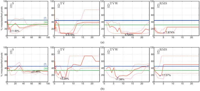
Per-formance are evaluated for a large range of values of the reg-ularization parameter λ (respectively, standard deviation σ for the local Gaussian smoothing based solution). To assess perfor-mance, misclassified pixel rate is evaluated as follows: The area with the largest median of estimated local regularity values is associated with the area of the original mask with largest regu-larity, the area with the second largest median of estimated local regularity values with the area of the original mask with second largest regularity value, and so on. Achieved results are reported in Fig. 2(a) (for h1 = 0.5 and h2 = 0.7) and (b) (h1 = 0.6 and

h2 = 0.7), respectively.

The three TV-based strategies (bΩTV, bΩTVWand bΩRMS) clearly outperform the local smoothing based solution bΩSover a large range of λ. The local smoothing procedure yields at best pixel misclassification rates of12% (Fig. 2(a)) and 28% (Fig. 2(b)). In contrast, the best results obtained with the TV-based strategies drop down to less than7% (Fig. 2(a)) and 12% (Fig. 2(b)) of misclassified pixels.

Among the TV-based algorithms, bΩTVW, relying on the joint estimation of regularity and weights, is the least sensitive to the precise selection of the regularization parameter λ and consis-tently yields the best performance. Notably, it outperforms all other procedures when the difference in regularity|h2− h1| is

small (Fig. 2(b)). For segmentation, the performance of the TV procedure (bΩTV) is similar to that of bΩTVW, yet bΩTV is more sensitive to the precise tuning of λ and yields large errors when λ _{is chosen too small or too large. For these cases, bΩ}TV de-tects only one area, while bΩTVWstill segments the texture into two areas. Solution bΩRMS also is more robust to the tuning of λ_{, compared to bΩ}TV_{, yet shows slightly decreased} misclassi-fication rates. Furthermore, bΩRMS has the practical advantage of being the only solution that does not require the practically cumbersome step of thresholding histograms (hence avoiding the empirical tuning of binning and smoothing parameters, for instance).

Fig. 2. Percentage of misclassified pixels as a function of penalty parameter λ (respectively, standard deviation σ forbΩS): median (solid red) and upper and lower quartile (dashed red) for ten realizations forΩbS,bΩTV,ΩbTVWandbΩRMS(from left to right, respectively). Subfigure (a):(h1, h2) = (0.5, 0.7); Subfigure

(b):(h1, h2) = (0.6, 0.7).

To illustrate, results obtained by each of the proposed pro-cedures for the value of λ (or σ) leading to a minimal clas-sification error (marked with symbols in Fig. 2) are reported in Fig. 3 when considering one randomly selected realiza-tion of multifracrealiza-tional Brownian fields with Q= 2 areas of constant regularity defined by (h1, h2) = (0.5, 0.7) (top) and

(h1, h2) = (0.6, 0.7) (bottom), respectively. Fig. 3(a) shows the

analyzed textures, illustrating that the two texture areas can not be distinguished visually. The local smoothing based labeling results bΩSare clearly the poorest, both for(h1, h2) = (0.5, 0.7)

and(h1, h2) = (0.6, 0.7). In contrast, all three TV-based

solu-tions bΩTV, bΩTVWand bΩRMSyield satisfactory performance. So-lution bΩTVW achieves the lowest misclassification error and is also visually the most convincing in terms of segmented regions, at the price though of the largest computational cost. Solution b

ΩTVshows only slightly larger misclassification rates sand may be preferred in certain applications for its significantly smaller computational cost. Solution bΩRMSshows larger misclassifica-tion rate when the difference in regularity decreases.

Moreover, the above analysis is complemented by the study of a situation with of Q= 3 areas (constant local regularities (h1, h2, h3) = (0.2, 0.4, 0.7)), with a more complex geometry,

including notably corners. The regularity mask, texture and la-beling results are illustrated in Fig. 4. The local smoothing solution bΩSfails to distinguish the three areas, yielding several disconnected domains, while all proposed TV based approaches correctly and satisfactorily detect the three distinct areas. Solu-tions bΩTVand bΩTVWshow similar results and again have slightly smaller classification error rates than bΩRMS. None of the pro-posed procedures recovers the two sharp corners of the original regularity mask. In particular, bΩTVand bΩTVWyield segmented areas with pronouncedly smooth borders.

In conclusion, the lowest misclassification rates are achieved by bΩTVW, followed by bΩTV and bΩRMS, and worst results are obtained with bΩS. The quality of the solutions obtained with the different strategies are related to their complexity, reflected by computation times. While bΩSis obtained in less than 1 second, the fastest TV based solution is bΩTV, with a computational time of about 10 seconds in our experiment, followed by bΩRMS with a 1-minute computational time. The solution achieving the best performance, bΩTVW, further requires around 3 minutes of computational time.

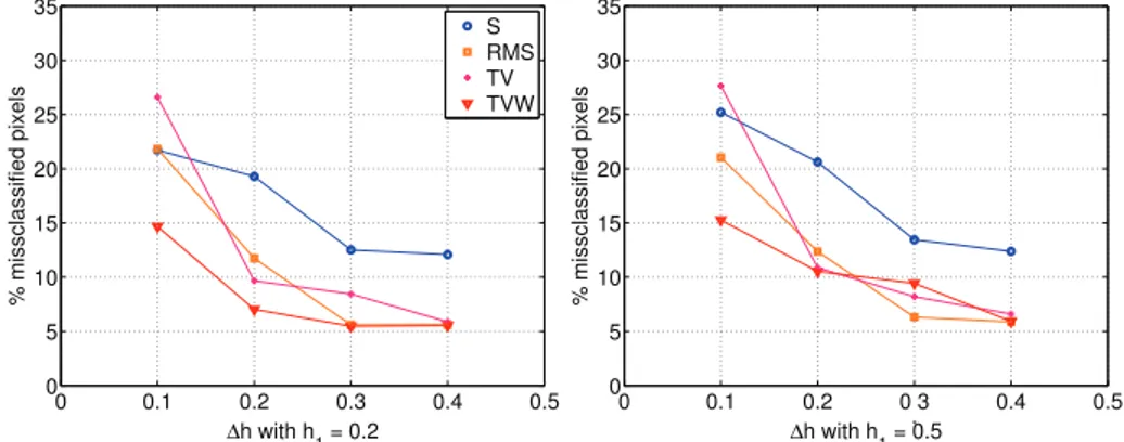
In order to evaluate more accurately the behaviour of the proposed method as a function of ∆h = h2− h1, additional

experiments are conducted in which h2 = h1+ ∆h for ∆h =

{0.1, 0.2, 0.3, 0.4}. Average (over ten realizations) pixel mis-classification rates for two different situations, h1 = 0.2 and

h1 = 0.5, are reported in Fig. 5 (the reported results are

ob-tained with values of λ that lead to best performance for the configurations). The results based on TV are displayed in hot colors (orange/pink/red) while the results obtained with the ba-sic smoothing is displayed in blue. As expected, the larger∆h, the better the performance for all methods. Moreover, the re-sults lead to the conclusion that the TV based approaches have superior performance and that the method that estimates si-multaneously the weights and the H¨older exponent, i.e., bΩTVW, yields overall smallest misclassification rates.

B. Comparisons With State-of-the-art Segmentation Procedures and Application to Real-World Textures

1) Comparisons with State-of-the-art Segmentation Proce-dures: Comparisons against two texture segmentation pro-cedures, chosen because considered state-of-the-art in the dedicated literature, are now discussed. The first approach [36]

Fig. 3. Results obtained with the different proposed solutions compared to a basic smoothing ofbh and the state-of-the-art texture segmentation approaches proposed in [36] and [7]. Top row: (h1, h2) = (0.5, 0.7); bottom row: (h1, h2) = (0.6, 0.7). (a) Data f . (b)bh_L.(c) [36]. (d) [7]. (e) Ωb

S

. (f) bΩTV. (g)ΩbTVW. (h)bΩRMS.

Fig. 4. Results of the labeling obtained with the different proposed solutions when Q= 3. (a) Data f . (b)bh

L. (c) [36]. (d) [7]. (e)bΩ S

. (f)bΩTV. (g)ΩbTVW. (h)bΩRMS.

Fig. 5. Results obtained with the different proposed solutions (in red) compared to a basic smoothing (in blue) as a function of∆h = h2− h1.

relies on a multiscale contour detection procedure using bright-ness, color and texture (using textons) information followed by the computation of an oriented watershed transform. The second approach [7] relies on Gabor coefficients as features followed by a feature selection procedure relying on a matrix factorization step. Results are reported in Figs. 2, 3, and 4 and unambiguously show that such approaches lead to much poorer segmentation performance as compared to the proposed TV-based procedures and appear ineffective for the segmentation of scale-free textures.

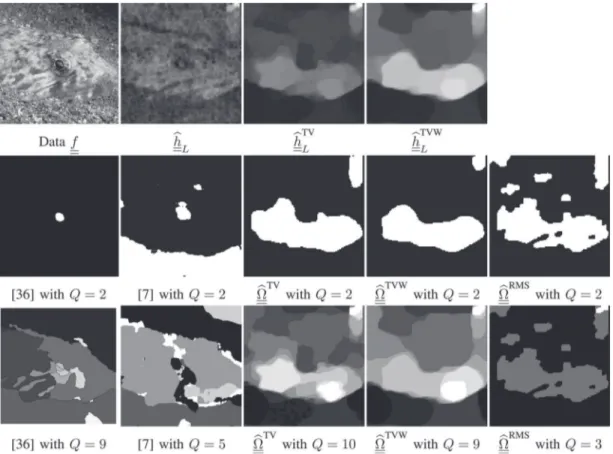
2) Real-World Textures: To assess the level of generality of the TV-based segmentation procedures, their performance are

quantified and compared on sample textures chosen randomly from a large database considered as reference in the dedicated literature, the Berkeley Segmentation Dataset.1No ground truth segmentation is available for that database. Samples are shown in Figs. 6 and 7 together with local regularity TV based esti-mation and segmentation procedure outcomes. For comparison, results achieved with the two state-of-the-art approaches in [36] and [7] are also displayed. For both examples, we provide two types of results: a 2-label segmentation result (Q= 2, Figs. 6 and 7, top rows) and the Q-labels segmentation results where,

Fig. 6. Experiments on real data: Image extracted from the Berkeley Segmentation Database.

for the state-of-the-art methods, Q had been tuned empirically in order to yield the visually most convincing solution, and where the solutions bΩTVand bΩTVW are deduced from bhTV_L and bhTVW_L (Figs. 6 and 7, bottom rows). For both examples, we observe that the outcomes of the segmentation resulting from TV approaches lead to satisfactory results: for Q= 2, a meaningful region is extracted, which is further refined when Q >2. When compar-ing to the state-of-the-art methods [36] and [7], we observe that all the methods lead to similarly meaningful yet not necessarily identical segmentation results. This is a satisfactory outcome regarding the general level of applicability of the proposed TV-based segmentation approaches since there is no reason a priori to believe that the samples in the Berkeley Segmentation Dataset are perfectly scale-free textures.

V. CONCLUSION ANDPERSPECTIVES

We proposed, to the best of our knowledge, the first fully op-erational nonparametric texture segmentation procedures that rely on the concept of local regularity. The segmentation pro-cedures was designed for the class of piecewise constant local regularity images. The originality of the proposed approach resided in the combination of wavelet leaders based local reg-ularity estimation and proximal solutions for minimizing the convex criterion underlying the segmentation problem. Three original and distinct proximal solutions were proposed, all re-lying on a TV penalization and proximal based resolution: TV denoising of local regularity estimates followed by thresholding for label determination; TV penalized joint estimation of local regularity and estimation weights followed by thresholding for label determination; direct labeling of local regularity estimates using a TV based partitioning strategy. The performance of the procedures was validated using stochastic Gaussian model processes with prescribed region-wise constant local regular-ity and illustrated using realistic model images with real-world textures. All proposed labeling procedures yielded satisfactory results. They significantly improved over labeling based directly on (smoothed) local regularity estimates, at the price though of increased computational costs. Procedure bhRMSfurther avoided to devise a detailed procedure for histogram thresholding, yet yielding slightly poorer results compared to bhTVW.

When constant regularity areas were labeled, regularity can be re-estimated a posteriori by averaging within each area the X(a, k) prior to performing linear regressions [27].

The proposed procedures are currently being used for the analysis of biomedical textures, with encouraging preliminary results. Comparisons with alternative texture characterization features, such as local entropy rates, are under investigation.

Future work will include investigating in how far the pro-posed approach can be adapted to handle different regularity models, such as images with piecewise smooth local regularity. Furthermore, the analysis of textures from real-world applica-tions would benefit from substituting piecewise constant H¨older exponents with piecewise constant multifractal spectra, provid-ing richer and more realistic models, at the price, yet, of more severe estimation and segmentation issues.

REFERENCES

[1] R. M. Haralick, “Statistical and structural approaches to texture,” Proc.

IEEE, vol. 67, no. 5, pp. 786–804, May 1979.

[2] M. M. Galloway, “Texture analysis using gray level run lengths,” Comput.

Graph. Image Process., vol. 4, pp. 172–179, 1975.

[3] K. Deguchi, “Two-dimensional auto-regressive model for analysis and synthesis of gray-level textures,” in Proc. 1st Int. Symp. Sci. Form, 1986, pp. 441–449.

[4] R. L. Kashyap, R. Chellappa, and A. Khotanzad, “Texture classification using features derived from random field models,” Pattern Recog. Lett., vol. 1, pp. 43–50, 1982.

[5] Y. Stitou, F. Turcu, Y. Berthoumieu, and M. Najim, “Three-dimensional textured image blocks model based on Wold decomposition,” IEEE Trans.

Signal Process., vol. 55, no. 7, pp. 3247–3261, Jul. 2007.

[6] P. Perona and J. Malik, “Preattentive texture discrimination with early vision mechanisms,” J. Opt. Soc. Amer. A., vol. 7, no. 5, pp. 924–932, 1990.

[7] J. Yuan, D. Wang, and A. M. Cheriyadat, “Factorization-based tex-ture segmentation,” IEEE Trans. Image Process., vol. 24, no. 11, pp. 3488–3496, Nov. 2015.

[8] C. Bouman and M. Shapiro, “A multiscale random field model for Bayesian image segmentation,” IEEE Trans. Image Process., vol. 3, no. 2, pp. 162–177, Mar. 1994.

[9] M. Unser, “Texture classification and segmentation using wavelet frames,” IEEE Trans. Image Process., vol. 4, no. 11, pp. 1549–1560, Nov. 1995.

[10] M. S. Crouse, R. D. Nowak, and R. G. Baraniuk, “Wavelet-based statisti-cal signal processing using hidden Markov models,” IEEE Trans. Signal

Process., vol. 46, no. 4, pp. 886–902, Apr. 1998.

[11] S. Mallat, A Wavelet Tour of Signal Processing. San Diego, CA, USA, Academic, 1997.

[12] X. Guofang, M. Brady, J. Noble, and Z. Yongyue, “Segmentation of ul-trasound B-mode images with intensity inhomogeneity correction,” IEEE

Trans. Med. Imag., vol. 21, no. 1, pp. 48–57, Jan. 2002.

[13] M. Pereyra, N. Dobigeon, H. Batatia, and J.-Y. Tourneret, “Segmentation of skin lesions in 2-D and 3-D ultrasound images using a spatially coherent generalized Rayleigh mixture models,” IEEE Trans. Med. Imag., vol. 31, no. 8, pp. 1509–1520, Aug. 2012.

[14] K. Ni, X. Bresson, T. F. Chan, and S. Esedoglu, “Local histogram based segmentation using the Wasserstein distance,” Int. J. Comput. Vis., vol. 84, no. 1, pp. 97–111, 2009.

[15] B. B. Mandelbrot, The Fractal Geometry of Nature. New York, NY, USA: Freeman, 1983.

[16] K. Falconer, Fractal Geometry: Mathematical Foundations and

Applica-tions. Hoboken, NJ, USA: Wiley, 2004.

[17] R. Lopes, P. Dubois, I. Bhouri, M. H. Bedoui, S. Maouche, and N. Betrouni, “Local fractal and multifractal features for volumic texture characteriza-tion,” Pattern Recog., vol. 44, no. 8, pp. 1690–1697, 2011.

[18] S. G. Roux, M. Clausel, B. Vedel, S. Jaffard, and P. Abry, “Self-similar anisotropic texture analysis: The hyperbolic wavelet transform contri-bution,” IEEE Trans. Image Process., vol. 22, no. 11, pp. 4353–4363, Nov. 2013.

[19] C. L. Benhamou et al., “Fractal analysis of radiographic trabecular bone texture and bone mineral density: Two complementary parameters re-lated to osteoporotic fractures,” J. Bone Mineral Res., vol. 16, no. 4, pp. 697–704, 2001.

[20] P. Kestener, J. Lina, P. Saint-Jean, and A. Arneodo, “Wavelet-based multi-fractal formalism to assist in diagnosis in digitized mammograms,” Image

Anal. Stereol., vol. 20, no. 3, pp. 169–175, 2004.

[21] Q. Guo, J. Shao, and V. F. Ruiz, “Characterization and classification of tumor lesions using computerized fractal-based texture analysis and support vector machines in digital mammograms,” Int. J. Comput. Assisted

Radiol. Surgery, vol. 4, no. 1, pp. 11–25, 2009.

[22] R. Lopes and N. Betrouni, “Fractal and multifractal analysis: A review,”

Med. Image Anal., vol. 13, pp. 634–649, 2009.

[23] S. G. Roux, A. Arneodo, and N. Decoster, “A wavelet-based method for multifractal image analysis. III. Applications to high-resolution satellite images of cloud structure,” Eur. Phys. J. B, vol. 15, no. 4, pp. 765–786, 2000.

[24] P. Abry, S. Jaffard, and H. Wendt, “When Van Gogh meets Mandelbrot: Multifractal classification of painting’s texture,” Signal Process., vol. 93, no. 3, pp. 554–572, 2013.

[25] P. Abry et al., “Multiscale anisotropic texture analysis and classification of photographic prints,” IEEE Signal Process. Mag., vol. 32, no. 4, pp. 18–27, Jul. 2015.

[26] S. Jaffard, “Wavelet techniques in multifractal analysis,” in Fractal

Geom-etry and Applications: A Jubilee of Benoˆıt Mandelbrot, M. Lapidus and M. van Frankenhuijsen Eds. Providence, RI, USA: AMS, 2004, vol. 72, no. 2, pp. 91–152.

[27] H. Wendt, P. Abry, and S. Jaffard, “Bootstrap for empirical multifractal analysis,” IEEE Signal Process. Mag., vol. 24, no. 4, pp. 38–48, Jul. 2007. [28] H. Wendt, S. G. Roux, P. Abry, and S. Jaffard, “Wavelet leaders and bootstrap for multifractal analysis of images,” Signal Process., vol. 89, no. 6, pp. 1100–1114, 2009.

[29] N. Pustelnik, H. Wendt, and P. Abry, “Local regularity for texture segmen-tation: Combining wavelet leaders and proximal minimization,” in Proc.

Int. Conf. Acoust., Speech Signal Process., Vancouver, Canada, May 2013, pp. 5348–5352.

[30] O. Pont, A. Turiel, and H. Yahia, “An optimized algorithm for the evalu-ation of local singularity exponents in digital signals,” in Proc.

Combina-torial Image Anal., 2011, pp. 346–357.

[31] C. Nafornita, A. Isar, and J. D. B. Nelson, “Regularised, semi-local hurst estimation via generalised lasso and dual-tree complex wavelets,” in Proc.

Int. Conf. Image Process., Paris, France, Oct. 2014, pp. 2689–2693. [32] N. Pustelnik, P. Abry, H. Wendt, and N. Dobigeon, “Inverse problem

formulation for regularity estimation in images,” in Proc. Int. Conf. Image

Process., Paris, France, Oct. 2014, pp. 6081–6085.

[33] J. D. B. Nelson, C. Nafornta, and A. Isar, “Semi-local scaling exponent estimation with box-penalty constraints and total-variation regularization,”

IEEE Trans. Image Process., vol. 25, no. 6, pp. 3167–3181, Apr. 2016. [34] T. Chan, S. Esedoglu, and M. Nikolova, “Algorithms for finding global

minimizers of image segmentation and denoising models,” SIAM J. Appl.

Math., vol. 66, no. 5, pp. 1632–1648, 2006.

[35] T. Pock, A. Chambolle, D. Cremers, and B. Horst, “A convex relaxation approach for computing minimal partitions,” in Proc. IEEE Conf. Comput.

Vis. Pattern Recog., Miami, FL, USA, 20–25 Jun. 2009, pp. 810–817. [36] P. Arbelaez, M. Maire, C. Fowlkes, and J. Malik, “Contour detection

and hierarchical image segmentation,” IEEE Trans. Pattern Anal. Mach.

Intell., vol. 33, no. 5, pp. 898–916, May 2011.

[37] P. Abry, P. Flandrin, M. S. Taqqu, and D. Veitch, “Wavelets for the analysis, estimation and synthesis of scaling data,” in Self-Similar Network Traffic

and Performance Evaluation, K. Park and W. Willinger, Eds. Hoboken, NJ, USA: Wiley, 2000, pp. 39–88.

[38] A. Ayache, S. Cohen, and J. L´evy Vehel, “The covariance structure of multifractional Brownian motion, with application to long range depen-dence,” in Proc. Int. Conf. Acoust., Speech Signal Process., Dallas, TX, USA, Mar. 2000, pp. 3810–3813.

[39] L. Rudin, S. Osher, and E. Fatemi, “Nonlinear total variation based noise removal algorithms,” Physica D, vol. 60, no. 1, pp. 259–268, 1992. [40] A. Chambolle, “An algorithm for total variation minimization and

appli-cations,” J. Math. Imag. Vis., vol. 20, no. 1/2, pp. 89–97, 2004.

[41] L. Condat, “A primal-dual splitting method for convex optimization in-volving Lipschitzian, proximable and linear composite terms,” J. Optim.

Theory Appl., vol. 158, no. 2, pp. 460–479, 2013.

[42] P. L. Combettes and V. R. Wajs, “Signal recovery by proximal forward-backward splitting,” Multiscale Model. Simul., vol. 4, no. 4, pp. 1168–1200, 2005.

[43] H. H. Bauschke and P. L. Combettes, Convex Analysis and Monotone

Operator Theory in Hilbert Spaces. New York, NY, USA: Springer, 2011. [44] P. L. Combettes and J.-C. Pesquet, “Proximal splitting methods in signal processing,” in Proc. Fixed-Point Algorithms Inverse Problems Sci. Eng., H. H. Bauschke, R. Burachik, P. L. Combettes, V. Elser, D. R. Luke, and H. Wolkowicz, Eds. New York, NY, USA: Springer-Verlag, 2010, pp. 185–212.

[45] N. Parikh and S. Boyd, “Proximal algorithms,” Found. Trends Optim., vol. 1, no. 3, pp. 123–231, 2014.

[46] B. C. V˜u, “A splitting algorithm for dual monotone inclusions involving cocoercive operators,” Adv. Comput. Math., vol. 38, pp. 667–681, 2011. [47] P. L. Combettes, J.-C. Condat, L. Pesquet, and B. C. V˜u, “A

forward-backward view of some primal-dual optimization methods in image re-covery,” presented at the Proc. Int. Conf. Image Processing, Paris, France, Oct. 2014.

[48] N. Komodakis and J.-C Pesquet, “Playing with duality: An overview of recent primal-dual approaches for solving large scale optimization prob-lems,” IEEE Signal Process. Mag., vol. 32, no. 6, pp. 31–54, Nov. 2015. [49] G. Peyr´e and J. Fadili, “Group sparsity with overlapping partition

func-tions,” in Proc. Eur. Signal Process. Conf., Barcelona, Spain, Aug. 2011, pp. 303–307.

[50] P. L. Combettes and J.-C. Pesquet, “A proximal decomposition method for solving convex variational inverse problems,” Inverse Problems, vol. 24, no. 6, 2008, Art. no. 065014.

[51] S. Theodoridis, K. Slavakis, and I. Yamada, “Adaptive learning in a world of projections,” IEEE Signal Process. Mag., vol. 28, no. 1, pp. 97–123, Jan. 2011.

[52] M. Kass, A. Witkin, and D. Terzopoulos, “Snakes: Active contour models,”

Int. J. Comput. Vis., vol. 1, no. 4, pp. 321–331, 1988.

[53] D. Mumford and J. Shah, “Optimal approximations by piecewise smooth functions and associated variational problems,” Commun. Pure Appl.

Math., vol. 42, pp. 577–685, 1989.

[54] V. Caselles, R. Kimmel, and G. Sapiro, “Geodesic active contours,” Int. J.

Comput. Vis., vol. 22, no. 1, pp. 61–79, 1997.

[55] Y. Boykov and M.-P Jolly, “Interactive graph cuts for optimal boundary & region segmentation of objects in ND images,” in Proc. IEEE Int. Conf.

Comput. Vis., 2001, pp. 105–112.

[56] A. Chambolle, D. Cremers, and T. Pock, “A convex approach to minimal partitions,” SIAM J. Imag. Sci., vol. 5, no. 4, pp. 1113–1158, 2012. [57] D. Cremers, P. Thomas, K. Kolev, and A. Chambolle, “Convex

relax-ation techniques for segmentrelax-ation, stereo and multiview reconstruction,” in Markov Random Fields for Vision and Image Processing, A. Blake, P. Kohli, and C. Rother, Eds. Boston, MA, USA: MIT Press, 2011. [58] S. Hiltunen, J.-C. Pesquet, and B. Pesquet-Popescu, “Comparison of two

proximal splitting algorithms for solving multilabel disparity estimation problems,” in Proc. Eur. Signal Process. Conf., Bucharest, Romania, Aug. 2012, pp. 1134–1138.

Nelly Pustelnik (S’08–M’11) received the Ph.D. degree in signal and image

processing from the Universit´e ParisEst, Marne-la-Vall´ee, France, in 2010. From 2010 to 2011, she was a Postdoctoral Research Associate in the Laboratoire IMS, Universit´e de Bordeaux, Bordeaux, France, working on the topic of tomographic reconstruction from a limited number of projections. Since 2012, she has been a CNRS Researcher with the Signal Processing Team, Laboratoire de Physique de l’ENS de Lyon. Her research interests include inverse problems, nonsmooth convex optimization, mode decomposition, and texture analysis.

Herwig Wendt received the M.S. degree in electrical engineering and

telecom-munications from the Vienna University of Technology, Austria, in 2005, and the Ph.D. degree in physics and signal processing from the Ecole Normale Suprieure de Lyon, Lyon, France, in 2008. From 2008 to 2011, he was a Postdoctoral Re-search Associate in the Department of Mathematics and the Geomathematical Imaging Group, Purdue University, West Lafayette, IN, USA. Since 2012, he has been a Tenured Research Scientist at the Centre National de Recherche Scientifique, Signal and Communications Group, IRIT Laboratory, University of Toulouse. He is also an Affiliated Faculty Member of the TeSA Laboratory.

Patrice Abry received the degree of Professeur-Agr´eg´e de Sciences Physiques

from Ecole Normale Sup´erieure de Cachan, Cachan, France, in 1989 and the Ph.D. degree in physics and signal processing from the Universit´e Claude-Bernard University in Lyon, Villeurbanne, France, in 1994. He is a CNRS Senior Scientist, at the Physics Department, Ecole Normale Sup´erieure de Lyon, in charge of the Signal, systems, and Physics research team. He au-thored a book in French on wavelet, scale invariance, and hydrodynamic turbulence and is the coeditor of a book entitled “Scaling, Fractals and

Wavelets” (Hoboken, NJ, USA: Wiley, 2013). His current research inter-ests include wavelet-based analysis and modeling of scaling phenomena and related topics (self-similarity, stable processes, multifractal, 1/f processes, long-range dependence, local regularity, infinitely divisible cascades, and so on). He has interests for real-world applications, hydrodynamic turbu-lence, computer network teletraffic, or heart rate variability. He received the AFCET-MESR-CNRS prize for best Ph.D. in Signal Processing for the years 93–94.

Nicolas Dobigeon (S’05–M’08–SM’13) was born in Angoulˆeme, France, in

1981. He received the engineering degree in electrical engineering from EN-SEEIHT, Toulouse, France, and the M.Sc. degree in signal processing from INP Toulouse, Toulouse, France, both in 2004, the Ph.D. degree and the Habilitation `a Diriger des Recherches in signal processing from INP Toulouse in 2007 and 2012, respectively.

From 2007 to 2008, he was a Postdoctoral Research Associate in the Department of Electrical Engineering and Computer Science, University of Michigan, Ann Arbor, MI, USA. Since 2008, he has been with INP-ENSEEIHT Toulouse, University of Toulouse, where he is currently an Associate Professor. He conducts his research within the Signal and Com-munications Group, IRIT Laboratory, and he is also an Affiliated Fac-ulty Member of the TeSA Laboratory. His recent research interests in-clude statistical signal and image processing, with a particular interest in Bayesian inverse problems with applications to remote sensing and biomedical imaging.