North American ground surface temperature histories : a contribution to the PAGES2k North American project

- -

-U IVERSITÉ DU QUÉBEC À MO TRÉAL

ORTH AMERICAN GROUND SURFACE TEMPERATURE HISTORIES: A

CO TRIBUTIO TO THE PAGES2K NORTH AMERICAN PROJECT

THESIS

PRESENTED

AS PARTIAL REQUIREMENT

OF THE MASTERS OF ATMOSPHERIC SCIE CES

BY

FER ANDOJAUMESANTERO

NOVEMBER 2016

-UNIVERSITÉ DU QUÉBEC À MONTRÉAL Service des bibliothèques

Avertissement

La diffusion de ce mémoire se fait dans le respect des droits de son auteur, qui a signé le formulaire Autorisation de reproduire et de diffuser un travail de recherche de cycles supérieurs (SDU-522 - Rév.03-2015). Cette autorisation stipule que «conformément à l'article 11 du Règlement no 8 des études de cycles supérieurs, [l'auteur] concède à l'Université du Québec à Montréal une licence non exclusive d'utilisation et de publication de la totalité ou d'une partie importante de [son] travail de recherche pour des fins pédagogiques et non commerciales. Plus précisément, [l'auteur] autorise l'Université du Québec à Montréal à reproduire, diffuser, prêter, distribuer ou vendre des copies de [son] travail de recherche à des fins non commerciales sur quelque support que ce soit, y compris l'Internet. Cette licence et cette autorisation n'entraînent pas une renonciation de [la] part [de l'auteur] à [ses] droits moraux ni à [ses] droits de propriété intellectuelle. Sauf entente contraire, [l'auteur] conserve la liberté de diffuser et de commercialiser ou non ce travail dont [il] possède un exemplaire.»

UNIVERSITÉ DU QUÉBEC À MONTRÉAL

HISTOIRE DE LA TEMPÉRATURE À LA SURFACE DU SOL DE L'AMÉRIQUE DU NORD: UNE CONTRIBUTIO AU PROJET PAGES

NAM2K

MÉMOIRE PRÉSENTÉ

COMME EXIGE CE PARTIELLE

DE LA MAÎTRISE EN SCIE CES DE L'ATMOSPHÈRE

PAR

FERNANDOJAUMESANTERO

ACK OWLEDGEMENTS

In first place, I have to thank my thesis directors, Dr. Hugo Beltrami, Dr. J

ean-Claude Mareschal and Dr. Laxmi Sushama for giving me the opportunity to make

this work pos ible.

Furthermore, I would like to thank my office colleages and friends Ignacio and

Lidia for the great times we passed together. Thank you to Hugo Beltrami and

Jean-Claude Mareschal for guiding me through the learni~g process of interesing

topics such as paleoclimate and climate change as well as the technical advices

in order to reconstruct and assess the climate histories obtained from subsurface

thermal profiles.

My recognitions to the UQÀM sciences faculty for its financial support as well

as the NSERC CREATE training program in climate sciences. This CREATE

(TPCS) training program is administered at Saint Francis Xavier University with

the cooperation of UQÀM among other universities. This CREATE TPCS is

funded by the atural Sciences and Engineering Research Council of Canada.

Moreover, I also want to thank the Geotop Research Centre in Geochemistry and Geodynamics for all the activities and students congresses that I was able to

participate.

Finally, I would like to give thanks to all my friends and family, pecially my mother Marisa, my sister Clara and my "chief commander" Carolyne. Thank you

for supporting and trusting me, without your effort this adventure would not had

been possible.

~---

----FOREWORD

The research work presents, integrally the masters thesis which I submitted the

summer of 2016 in the Department of Earth and Atmospheric Sciences at

Uni-versité du Québec à Montréal as partial requirement of the master of sciences in

atmospheric sciences.

This research thesis is composed by a general introduction of the topic, followed by two articles and a general conclusion. The thesis is written in english with a

french résumé attached. With the goal of submitting articles to scientific journals,

they are presented to satisfy the criteria for international rules of publication, with

summaries at the beginning and the tables and figures at the end.

The first article's title is North American database for borehole temperature re

-constructions and the second article's title is North American regional climate

reconstruction from Gmund Surface Temperature Histories. The writing of these

articles resulted from the collaboration between my thesis co-directors, Dr.

Jean-Claude Mareschal professor of geophysics in the Atmorpheric and Earth sciences

department at UQÀM and part of GEOTOP research center, and Hugo Beltrami who holds a Canada research Chair in Climate Dynamics at St. Francis Xavier University, he is an associate professor in the Department of Earth and

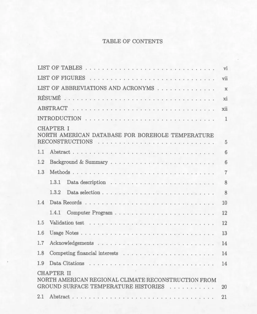
TABLE OF CO TENTS

LIST OF TABLES 0 v1

LIST OF FIGURES v11

LIST OF ABBREVIATIO SAND ACRO YMS x

RÉSUMÉ 0 0 Xl

ABSTRACT Dl

I TRODUCTION 1

CHAPTER I

NORTH AMERICAN DATABASE FOR BOREHOLE TEMPERATURE

RECONSTRUCTIONS 5

1.1 Abstract 0 0 0 0 0 0 0 0 0 0 6

1.2 Background & Summary 0 6

1.3 Methods 0 0 0 0 0 0 0 0 0 7 1.301 Data description 1.302 Data selection 0 1.4 Data Records 0 0 0 0 0 10401 Computer Program 0 8 8 10 12 1.5 Validation test 12 1.6 Usage Notes 0 0 13 1.7 Acknowledgements 14

1.8 Competing financial interests 14

1.9 Data Citations 0 0 0 0 o 14

CHAPTER II

ORTH AMERICAN REGlO AL CLIMATE RECO STRUCTIO FROM

GROU D SURFACE TEMPERATURE HISTORIES 20

2.2 Introduction . 2.3 Methodology

2.3.1 Temperature-depth equation .

2.3.2 Parametrization of the temperature anomaly .

2.3.3 Inversion . . . . . . . . . . . .

2.3.4 Subsurface temperature anomaly

2.3.5 Singular value decomposition

2.3.6 Forward model

2.3.7 Data . . . .

2.3.8 Data selection .

2.4 Results & discussion .

2.4.1 North-American ground surface temperature change .

2.4.2 Regional averages . . . . . . 2.4.3 Geographical representation 2.5 Conclusions 2.6 Appendix 1 2. 7 Acknowledgements CONCLUSION . . . APPE DIX A

A MILLE IAL RECO STRUCTIO

APPE DIX B

BOREHOLE TEMPERATURE PROFILE METADATA.

REFERE CES . . . . v 21 24 26 27 28 29 30 32 33 34 36 36 38 40 41 41 43 56 58 61 77

LIST OF TABLES

1.1 Data sources from where the temperature-depth profiles were taken. 15 2.1 Recorders useful for temperature histories. It presents their

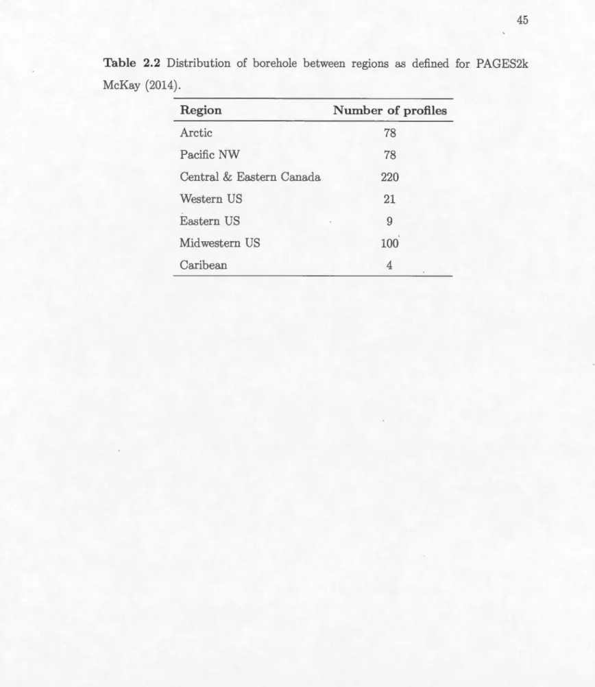
mini-mum resolution and maximum time range of reconstruction. . . . 44 2.2 Distribution of borehole between regions as defined for PAGES2k

McKay (2014). . . . . . . . . . . . . . . . . . . . . . . . . . . 45 2.3 Data sources where the temperature-depth profiles were taken. 46 B.1 Supplementary metadata of 510 BTPs suitable for climate

LIST OF FIGURES

Figure

1.1 Borehole CA-9308. Borehole temperature profile, the dots are the

temperature measurements T(z), the red line is the fit, obtained by

linear regression of the lower 100 meters, extrapolated to the

sur-facez= 0 and the blue lines represent two maximum steady states

related with the errors (in the intercept and slope) associated with

the method to ob tain the geothermal ste ad y state qaR( z) +Ta

.

reference temperature at the surface Ta is associated to the inter

-cept an the heat flux qa is related with the slope. The transient

perturbation Tt (green area) related with the climate signal is ob

-tained by the subtraction of the geothermal steady-state from the

Page

full profile. . . . . . . . . . . . . . . . . . . . . 16

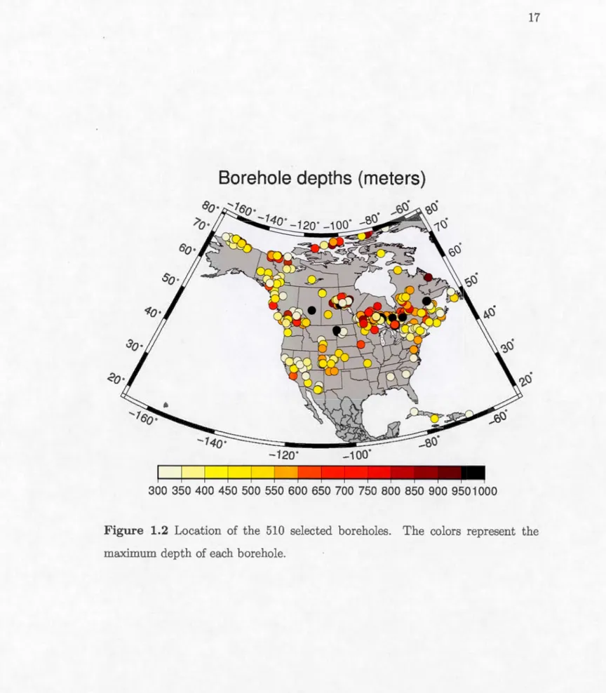
1.2 Location of the 510 selected boreholes. The colors represent the

maximum depth of each borehole. . . . . . . . . . . . . . . . 17

1.3 Ta(°C) & Latitude relation. Left: Linear regression of Ta. The least

square method fits with R2 _{= 83.1 %. Right: Surface interpolation}

map of Ta in degrees Celsius. . . . . . . . . . . . . 18

1.4 Conductivity of 453 boreholes. The colors represent the mean con

-ductivity in each borehole. . . . . . . . . . . . . . . . . . . . . . . 19

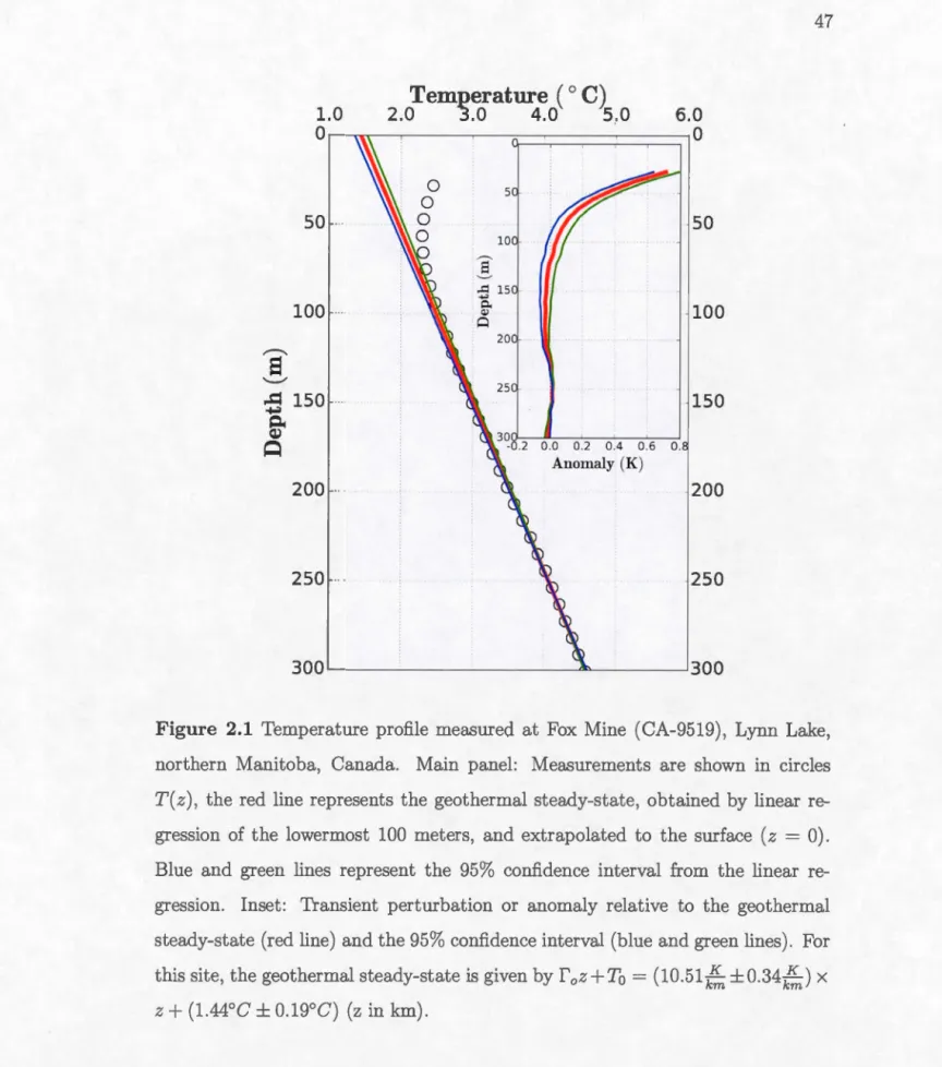
2.1 Temperature profile measured at Fox Mine (CA-9519), Lynn Lake,

northern Manitoba, Canada. Main panel: Measurements are shawn

in circles T(z), the red line represents the geothermal steady-state,

obtained by linear regression of the lowermost 100 meters, and ex

-trapolated to the surface (z = 0). Blue and green lines

repre-sent the 95% confidence interval from the linear regression.

In-set: Transient perturbation or anomaly relative to the geothermal

steady-state (red line) and the 95% confidence interval (blue and

green lines). For this site, the geothermal steady-state is given by

2.2 Ground surface temperature history for CA-9519 (Fox Mine, 1995). The red line represents the ground surface temperature history re-constructed from inversion. The blue and green lines are the GSTs for the anomalies estimated from the 95% uncertainty limits of the

Vlll

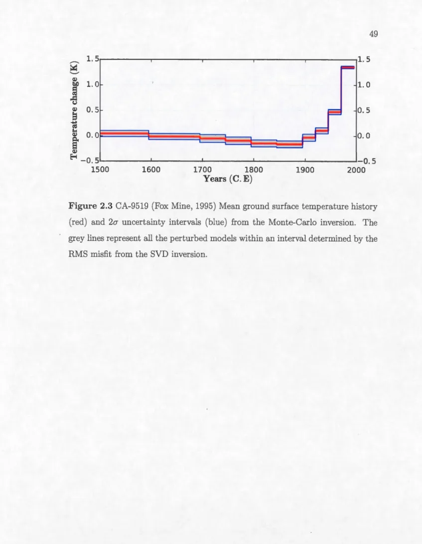
quasi steady-state profile. . . . . . . . . . . . . . . . 48 2.3 CA-9519 (Fox Mine, 1995) Mean ground surface temperature

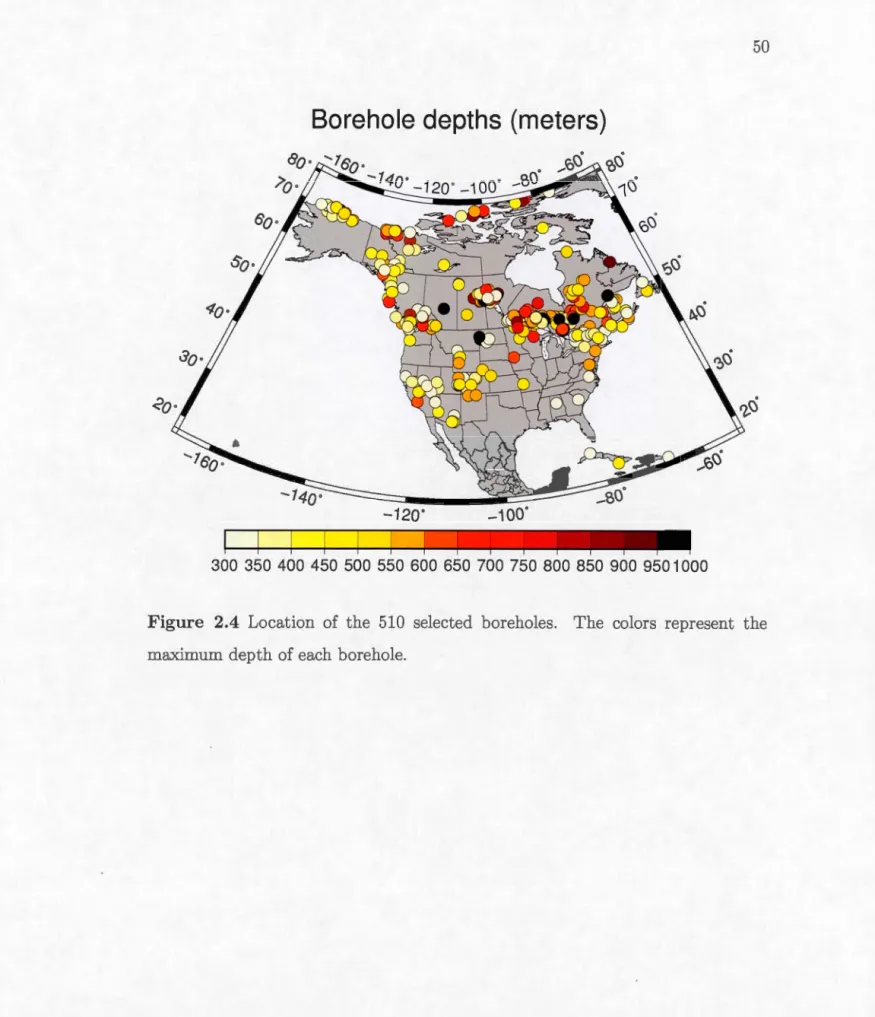
his-tory (red) and 20' uncertainty intervals (blue) from the Monte-Carlo inversion. The grey lines represent all the perturbed models within an interval determined by the RMS misfit from the SVD inversion. 49 2.4 Location of the 510 selected boreholes. The colors represent the

maximum depth of each borehole. . . . . . . . . . . . . . . . 50 2.5 Mean orth American ground surface temperature change (black).

Shown in blue are the 510 ground surface temperature reconstruc-tions inferred from the Monte Carlo inversion. . . . . . . . . . 51 2.6 Mean North American ground surface temperature history (blue)

and maximum temperature range of accepted models ( rv0.44 K) obtained from the Monte Carlo method (blue shade). Also shawn are proxy-based surface air temperature reconstruction for North America from 1500 to 2000 CE. All anomalies are displayed as departures from 1904-1980 mean. . .

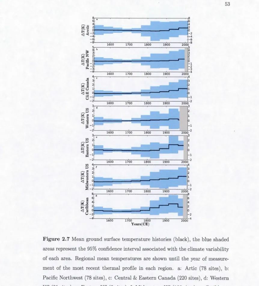
2. 7 Mean ground surface temperature histories (black), the blue shaded areas represent the 95% confidence interval associated with the di-mate variability of each area. Regional mean temperatures are shown until the year of measurement of the most recent thermal profile in each region. a: Artic (78 sites), b: Pacifie Northwest (78 sites), c: Central & Eastern Canada (220 sites), d: Western US (21 sites), e: Eastern US (9 sites), f: Midwestern US (100 sites), g:

52

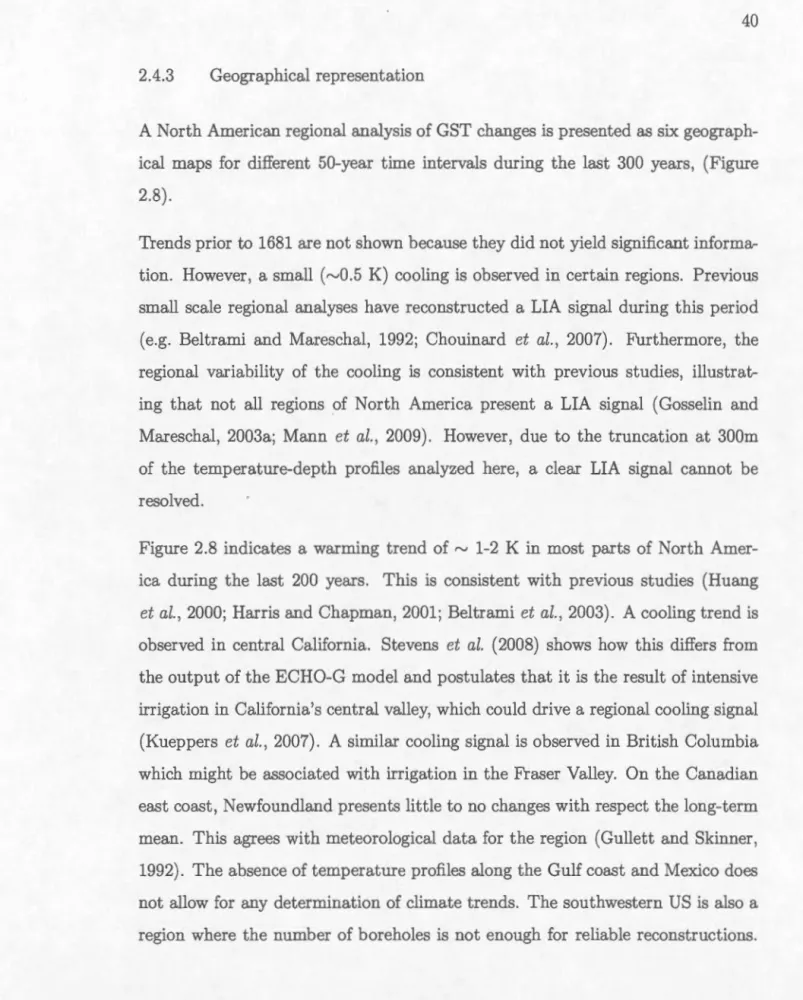
Caribbean ( 4 sites). . . . . . . . . . . . . . . . . . . . . 53 2.8 Spatial variability of the ground surface temperature variation (in

degrees Kelvin) from 1681 to 1980. Each panel shows a region-ally interpolated mean ground surface temperature over 50 years. The surface has been masked for zones without at least one datum within a radius of 400 km. Ground surface temperature changes are presented as departures from long-term mean surface temperatures prior to 1500 CE. . . . . . . . . . . . . . . . . . . . . . . . . . 54

2.9 Mean North American ground surface temperature histories for

dif-ferent parametrizations. Full inversions have been done for two

different time distributions: 10 time-steps using equation (2.15)

(orange) and 25 time-steps of 20 years each (red). Furthermore, it

has been added a mean ground surface temperature history (blue)

obtained from the reconstruction of the anomalies using the lin

-ear regression method. Its filtered version (black) was presented in

lX

Figure 2.5. . . . . . . . . . . . . . . . . . . . . . . . . . . . . 55

A.1 Millennial North American GST history (green line) compared with

North American GST reconstruction for the past 500 years (blue

line) presented in Chapter 2. The annual surface temperature

sim-ulation from GISS-E2-R (red line) has been added to the figure.

LIST OF ABBREVIATIONS AND ACRONYMS

BH Borehole

BTP Borehole Temperature Profile

CE Common Era

GST Ground Surface Temperature

GSTH Ground Surface Temperature History

LIA Little lee Age (1500-1800)

NAm Nor th America

NH Northern Hemisphere

PAGES Past Global Changes

SAT Surface Air Temperature

SQL Structured Query Language

SVD Singular Value Decomposition

RÉSUMÉ

Dans le cadre du projet PAGES NAm2k, 514 profils de température, mesurés dans des forages, ont été analysés pour le climat récent en l'Amérique du ord. Les profils thermiques sélectionnés ont été enregistrés dans une base de données SQL. Pour faciliter les comparaisons et afin d'examiner la même période de temps, les profils ont été tronqués à 300 m. Les histoires de la température à la surface du sol pour les 500 dernières annés ont été obtenues par inversion de l'anomalie de température en utilisant la méthode de décomposition en valeurs singulières afin d'obtenir les changements de température durant 10 intervalles de temps de durée variable. Les inversions ont été filtrées pour quatre valeurs singulières et les histoires ont été décalées dans le temps en fonction de l'année où les forages ont été mesurés. La température de surface de référence et le gradient thermique ont été calculés par régression linéaire pour les derniers 100 mètres avec un intervalle de confiance de 95%. De plus, une méthode de Monte Carlo a été appliquée afin de trouver un ensemble de solutions à l'intérieur d'une marge d'erreur donnée par la différence quadratique moyenne entre le modèle et les données. Les reconstructions ont ensuite été modélisées directement afin d'assurer qu'elles sont à l'intérieur de la marge d'erreur maximale. Une analyse régionale a été réalisée pour reconstruire les variations de température moyenne tous les 50 ans au cours des 5 derniers siècles. Les résultats des modèles acceptés, donnés par la température moyenne et l'erreur de 20' présentent, dans la plupart des cas, un réchauffement de 1°0 à 2.5°0 au cours des 100-150 dernières années.

MOTS-CLÉS: changement climatique, paléoclimatologie, histoires de la tempéra-ture à la surface du sol, réchauffement, PAGES2k

ABSTRACT

Within the framework of the PAGES Am2k project, 514 orth American tem-perature depth profiles were analyzed to infer recent climate changes. The selected profiles were saved inside a SQL data base. The ground surface temperature ( GST) histories for the last 500 years were reconstructed from the subsurface tempera-ture anomalies using a singular value decomposition (SVD) inversion that retains four principal components and takes into account time logging differences. Steady-state surface temperature and thermal gradient were estimated by linear regression for the lower 100 meters of the temperature profile, and climate induced subsur-face temperature anomalies were estimated as departures from the steady-state conditions. In addition, a Monte-Carlo method was applied to find the range of acceptable solutions within a maximum error interval between the forward mod-elled reconstruction and the profile. A regional analysis was performed for the last 5 centuries yielding mean temperature change every 50 years. The results, presented as the mean and 20" distance of 500 accepted models, show a warming by 1.0°C to 2.5°C during the post industrial era.

KEYWORDS: climate change, ground surface temperature histories, PAGES2k, paleoclimatology, warming.

I TRODUCTION

The climate of our planet is determined by the balance of incoming and outgoing radiation in the upper atmosphere. Weather and climate emerge from any energy imbalance which results from the difference between the energy absorbed by the atmosphere and the energy emmited to outer space (Hansen et al., 2005, 2011; von Schuckmann et al., 2016). Climate forcings are defined as natural or human induced perturbations of the energy balance originated outside the climate system. The oceans and the atmosphere, among other climate subsystem:;;, are sentistive to those changes in the energy budget which are translated in a sequence of climate changes such as global warming (Allan et al., 2014; Trenberth et al., 2014). With the present increase of the global mean temperature, an understanding of the past climate and its variability during the last millennium has become imperative in order to gain insights into present and future climate changes.

The key to understanding the impacts of human activity over the climate sys -tem resides in the ability to distinguish between its natural variability and the possible changes induced by human activity. General circulation models (GCMs) have become useful tools to forecast future climate trends under various scenarios defined by different climate forcings. However, GCMs must be compared with robust past climate reconstructions to asses their simulations and improve their outputs(Gonzalez-Rouco et al., 2009; PAGES 2k-PMIP3 group, 2015; Smith et al., 2015).

As meteorological records only cover a small fraction of the Earth's climatic his-tory, they are too short to give a longer perspective on climate variability. ev

-2

ertheles, climate-dependent natural phenomena provide an indirect approach to reconstruct and understand past global changes. Therefore, climate histories ob-tained from paleoclimate recorders are used to study past climate changes. It is the study of these proxy indicators that forms the foundation of paleoclimatology (2k Consortium, 2013).

Data records extracted from ice cores (Oeschger and Langway, 1989; Bauer et al., 2013; Thompson et al., 2013), tree rings (Douglass, 1919; Briffa et al., 1990; George and Ault, 2014), pollen (Davis et al., 2003; Viau et al., 2012; Jacques et al., 2015) and boreholes (Mareschal and Beltrami, 1992; Bodri and Cermak, 2007; Beltrami et al., 2014), among others, are commonly used for past elima te reconstructions. All of them have different resolutions and may be sentitive to different factors. For instance, tree ring reconstructions have better short temporal resolution(annual) than borehole temperature inversions (multidecadal), but due to standardization, long tree-ring chronologies may not reconstruct long-term climate variability prop-erly (Briffa and Osborn, 1999).

On the other hand, borehole climatology assumes that surface air temperature (SAT) and ground surface temperature GST are coupled, and their changes induce perturbations that propagate through the subsurface by heat conduction (Harris and Chapman, 1998a,b; Garcia-Garcia et al., 2016), neglecting the advection term. Temperature-depth profiles measured in boreholes have commonly been used by geophysicists to study the Earth's heat flux (Bullard, 1939; Benfield, 1939). In the 1930's, Hotchkiss and Ingersoll attempted to infer past climate from temperature-depth profiles (Hotchkiss and Ingersoll, 1934). It was only in the 1970s that sys-tematic studies to infer past climate from borehole temperature profiles (BTPs) were undertaken (Cermak, 1971; Sass et al., 1971; Beek, 1977). With the con-cern about warmer global temperatures, studies have become more widespread,

3

including local and global analyses (Beltrami et al., 1992; Clauser and Mareschal,

1995; Mareschal et al., 1999; Huang et al., 2000; Pickler et al., 2016b). Several regional analyses have been undertaken in orth America (Gosnold et al., 1997; Majorowicz et al., 2002; Chouinard et al., 2007) but none of them has analyzed the entire continent in detail. Following that line, the study presented in this

the-sis aims at filling this gap by performing a regional analysis of past GST changes

in Iorth America for the past 5 centuries.

The first part of the study was the collection of a database with thermal profiles

suitable for climate reconstructions. A data collection of thousands of thermal

profiles was accomplished in order to assess their quality. The main reason for

this data selection is that most of those profiles were measured for heat flux studies,

and might not be adequate for climate purposes. Reasons for rejection were for instance, the detection of ground water flow and conductivity changes that might

alter the climate signal recorded as a perturbation from the geothermal

steady-state, an insufficient depth range, less that 100 meters and deeper than 300 meters

for a reconstruction of the past 5 centuries). Selected borehole temperature profiles

were put in a public database and the whole process is described in the fust article

(Chapter 1), North American database for· borehole temperature reconstructions.

Furthermore, within the framework of PAGES2k project, more than 500 borehole temperature-depth profiles selected from orth America were analyzed to

recon-struct the GST histories for the past 5 centuries. Steady-state surface temperature

and thermal gradient were estimated by linear regression for the lower 100 meters

of the temperature profile, and climate induced subsurface temperature anomalies

were estimated as departures from the steady-state conditions. The GST

histo-ries for the past 500 years were reconstructed from the subsurface temperature

anomalies using a singular value decomposition (SVD) inversion. Additionally, a

max-4

imum subsurface anomaly error determined by the root mean square difference between the model and the data. A regional analysis was performed for the last

5 centuries yielding mean temperature change every 50 years. The GST history

results, presented as the mean and 95% confidence interval, show a warming by

1.0°C to 2.5°C during the post industrial era. These reconstructions span the

orth American continent and allow for the examination of regional trends. This

composes the second article NoTth AmeTican regional climate reconstruction from

Ground SuTface Temper-ature HistoTies which is a contribution for PAGES2k, and

will be published in Climate of the Past, Special Issue: Climate of the past 2000

years: global and Tegional syntheses. It is the base of this thesis (Chapter 2).

Finally, a GST reconstruction for the past 1000 years, obtained from boreholes truncanted at 500 meters, will be presented as an appendix where it is compared with the 500-year GST reconstruction studied in Chapter 2 as well as the surface

CHAPTER I

ORTH AMERICA DATABASE FOR BOREHOLE TEMPERATURE RECONSTRUCTIONS

Fernando Jaume-Santero1, Hugo Beltrami2•3, Jean-Claude Mareschal1

1_{Centre de Recherche en Géochimie et en Géodynamique (GEOTOP), Université} du Québec à Montréal, Montréal, Québec, Canada

2_{Climate & Atmospheric Sciences Institute and Department of Earth Sciences, St.} Francis Xavier University, Antigonish, Nova Scotia, Canada

3_{Centre pour l'étude et la simulation du climat à l'échelle régionale (ESCER),} Université du Québec à Montréal, Montréal, Québec, Canada

6

1.1 Abstract

Analyses of geothermal data from borehole temperature profiles are able to yield

reconstructions of low-frequency temporal variations of the ground surface

tem-perature. These ground surface temperature reconstructions form part of the

paleoclimatic network that is suitable for validation of climate model simulations.

Thus, we have increased the number of North American temperature depth pro-files useful for temperature reconstructions from 245 in Huang, Pollack and Shen (2000) to 510 in the present database. These data are in a public database

con-taining North American borehole temperature profiles deeper than 300 meters,

that are suitable to reconstruct recent (500 years) low-frequency climate trends.

1.2 Background & Summary

General circulation model (GCM) simulations are very useful to forecast future

climate projections under different predefined scenarios. However, because of the

limited resolution of GCMs, many significant climate-involved processes driving

at less than the GCM grid size scale are parameterized differently among model teams, therefore their outputs still have a large degree of uncertainty and they

need to be compared with real climate data to assess their robustness and validate

their outputs. As instrumental meteorological data are only available for the past 150 years, climate reconstructions for longer timescales require paleoclimatic data.

There is a wide diversity of paleoclimatic data within Earth's system such as tree

rings, ice cores, pollen, lake sediments, or borehole temperature profiles , that have

their own degree of spatial and temporal uncertainties. Paleoclimatic archives,

su ch as th ose kept by the National Climate Data Center at OAA, contain data

from these indirect climate recorders that allow for the reconstruction of past

7

In borehole climatology (Bodri and Cermak, 2007; Gonzalez-Rouco et al., 2009), it is assumed that surface air temperature (SAT) and ground surface tempera-ture (GST) are coupled(e.g. Harris and Chapman, 1998b, 2001). The changes in ground surface temperature propagate downward and are recorded as transient perturbations to the steady-state geothermal regime in the subsurface. Therefore, it is possible to estimate changes in ground surface temperature and infer past climate variations from the perturbations of the borehole temperature profiles

(BTPs) (e.g. Beltrami et al., 1992; Beltrami and Mareschal, 1993; Clauser and

Mareschal, 1995; Huang et al., 2000).

We present in a public database all the BTPs suitable for climate studies that can be used to perform a regional analysis of ground surface temperature histories for the past 500 years in North America. Our analysis will be included in the special volume of the PAGES NAm2k project along with other proxies to reconstruct the climate trends in orth America for the Common Era.

1.3 Methods

Assuming a homogeneous subsurface in absence of non-climatic perturbations, temperature increases linearly with depth. Thus, heat flux can be considered as "steady-state" with respect to the time scales of climatic surface variations. Thermal profiles measured in boreholes have commonly been used by

geophysi-cists to determine Earth's heat flux and estimate the geothermal 11

steady-state"

( e.g. Bullard, 1939; Benfield, 1939). However, perturbations of underground

tem-peratures by elima te variations at the surface are clear ly refiected in the thermal profile. These climate perturbations recorded in the subsurface must be extracted from the profile to infer past surface temperature trends. The quality of the profile for climate purposes will be determined by natural conditions at the location of

topog-8

raphy, or the hydrology, as well as requirements on the thermal profiles such as

the minimum depth. Thousands of North American BTPs were passed through a

selection process to assess whether they were suitable for climate reconstructions.

1.3.1 Data description

Temperature profiles measured in boreholes were obtained from the public databases

listed in the Data Citations section. Borehole datasets consists of a set of s

ub-surface temperatures T(z) and associated depths (Figure 1.1). The measurement

process consists of introducing a thermistor probe inside the borehole and tak

-ing measurements of the resistance at different depths ( usually beneath the water

table. Resistance (H1) is usually measured every 10 meters (sometimes 50 feet).

With the thermistor calibrated in the lab for the range of expected temperatures,

temperatures are determined with an estimated accuracy on the order of 20 mK

and a precision greater than 5 mK.

In addition to the BTP data, there are also metadata describing the features of the

borehole such as the location, the diameter of the hole, thermal conductivity, heat

production among many others. Information useful for climate reconstructions

was included in the metadata table. See the Data Records section for more details.

Information concerning the original contributors, is listed in the database under

contact for each BTP. When a contact name could not be found, the contact is

listed as unknown.

1.3.2 Data selection

Many BTPs, published for heat flow studies, are available in public datasets. A

list of such datasets for orth American thermal profiles is provided in Table 1.1.

However, not all of these profiles are suitable for climate reconstructions. Thus,

9

climate studies. There are many potential sources of non-climatic perturbations

of the BTP that can affect the extraction of the geothermal steady-state and

the reconstruction of past temperature changes at the surface. Therefore, several conditions are defined to ensure that the dataset contains dean thermal profiles

without non climatic disturbances. The conditions that we have set are the fol

-lowing:

1. Depth range: U seful profiles must be deeper than 300 meters in or der to be

able to reconstruct for at least the past 500 years. The first measurement

must have a minimum depth of 95 meters to be able to properly define the

temperature perturbation of the past 100 years which usually dominates the

climate signal.

2. Number of measurements: Each profile must contain at least 10 measure-ments.

3. General check: Temperature-depth profiles are plotted as in Figure 1.1 to

eliminate profiles that exhibit obvious non-climatic disturbances such as

water flow, or abrupt conductivity changes.

4. Surface conditions near the borehole: Many sources of non climatic

pertur-bations can be observed at the surface ( Chouinard and Mareschal, 2007).

Recent deforestation can induce a local warming signal that is not due to

climate change (Lewis and Wang, 1998). Other surface conditions affecting the temperature profile include topography (higher elevation producing an apparent warming signal), the presence of lake (profiles from holes inclined

toward a lake giving an apparent cooling signal in Canada). U nfortunately, surface conditions have not been documented for the majority of the heat

flow studies before 1980, and the selection was possible only for the most

10

Consequently, after selecting profiles from sever al datasets (Table 1.1), we only

re-tained a small fraction of them (in total 510), and included them in this database.

Their locations are shawn on a map (Figure 1.2).

The distribution of the retained profiles is not uniform across orth America. The

Canadian Shield is very well sampled (at least its southern part) because it was

the target of heat flow studies of the continental lithosphere, and because mining

exploration hales are available to measure temperature depth profiles in crystalline

rocks. Suitable profiles are absent from the Gulf coast region including Oklahoma

and Texas. Sedimentary basins are often affected by water flow and thermal

convection in the permeable sediments. Furthermore, temperature measurements

in oil wells are made out of equilibrium during drilling. Wells that are not put in

production are cemented to avoid contamination of aquifers, and not accessible

for measurements. Very few profiles are found in the southwestern United States

where many heat flux measurements have been made. In the Basin and Range

Province, where heat flow is very high, shallow hales are suffi.cient to define a

high temperature gradient. Furthermore most measurements in the Southwestern

US were made in hales drilled in basins strongly affected by thermal convection.

There is also a lack of useful deep profiles in Mexico and the Caribbean.

1.4 Data Records

The database presents 510 BTPs suitable for climate reconstruction and a

meta-data table containing useful information about each of them. They are publicly

available in Figshare, DOl: 10. 6084/m9. figshare. 2062140, and they can be

downloaded from

https: 1 /figshare. com/s/Oa1d213c3814024c4333. They can be found in two

11

are efficiently loaded with different research environments such as MATLAB,

Jupyter/Python or R.

The CSV dataset is organized to be loaded with a spreadsheet.

The metadata table (METADATA.CSV) contains the following columns,

• N ame: Borehole IDs.

• Longitude: Coordinate X longitude (decimalized)

• Latitude: Coordinate Y latitude ( decimalized)

• Logging Year: The year(s) when the borehole was measured.

• Contact: Person or group who logged the profile.

• Country: The country where the borehole was drilled.

• Thermal conductivity

• Max. Depth: Maximum logged depth.

• Data number: umber of measurements for each BTP.

The coordinates have been decimalized. The accuracy of the location depend on the age of the measurement. For the the oldest data the location is accurate to

a minute; for the recent data, the location accuracy is better than a tenth of a

second. Each temperature profile is contained in an individual CSV file identified with the borehole name.

12

The data are in two columns:

• Depth rn: The depth (z) in meters.

• Temperature Celsius: The temperature (T(z)) in degrees Celsius.

The same data scheme is followed for the profiles in the TABULAR database. Their metadata appear as comments (preceded by #) in the same file as the temperature-depth measurements.

1.4.1 Computer Program

Short computer programs are included in the data package. They show examples of how to load the profiles and metadata contained in the database. The example codes are: load_data.m Matlab/Octave code that loads the temperature-depth profile from CSV files, load _ data.py Python 3 script that loads the temperature-depth profile as well as the metadata for a given borehole in the TABULAR database and meta_panda.ipynb, !python code that loads the entire metadata file, using Pandas, the python data analysis library. Furthermore, CSV is a multi-platform format that can be directly loaded by spreadsheet-based programs such as EXCEL or Open Office.

1.5 Validation test

A te t was performed to check the consistency of the profiles truncated at 300 me-ters. Reference surface temperatures

(Ta)

13

1.6 Usage otes

This borehole database is published to be used for a orth American regional

analysis from ground surface temperature histories using temperature-depths pro

-files suitable for climate reconstructions. Several methods for inversion of these data have been proposed by different research groups: Backus-Gilbert method (Vasseur et al., 1983), functional space inversion (Shen and Beek, 1991), singu-lar value decomposition (Mareschal and Beltrami, 1992), Monte-Carlo method

(Mareschal et al., 1999). A discussion and comparison between sorne of the

meth-ods can be found in Beek et al. (1992). The same methods can also be applied for

simultaneous inversion of all the data from a given region. Computer programs implementing the inversion algorithms can be requested from the researchers. The database could also be useful to study spatial differences of conductivity in orth America. Conductivities obtained from 453 boreholes vary from 0.87 W jmK to 7.23 W /mk as shown in Figure 1.4. This is a parameter that takes very different values in different climate models. As a first approach, no regional conductivity patterns are discerned. However, a more complete study of the spatial

distribu-tion of thermal conductivities could be done by adding those boreholes shallower

14

1.7 Acknowledgements

Many researchers have been involved in the collection of the data included in this compilation. A probably incomplete list includes A. Judge, A. Taylor, A.H. A. Beek, Lachenbruch, A.M. Jessop, D.D. Blackwell, D. Chapman, E.R. Decker , F. Birch, F.E. Urban, G. Clow, H.N. Pollack, J. Heine, J. Majorowicz, C. Jaupart, J.C. Mareschal, G. Bienfait, C. Pinet, L. Guillou, F. Rolandone, C. Gasselin, F. Levy, C. Phaneuf, C. Pickler, C. Chouinard, J.H. Sass, K. Wang, L. Larry, M. Severson, P. Morgan, R. Roy, R. Scatollini, R. . Harris, S.R. Durrans, T. Lewis, V. Cermak, W.D. Gosnold, W.H. Benkowski, W.H. Diment. We apologize to those who have been left out. This work was supported by grants from the N atur al Sciences and Engineering Research Co un cil of Canada Discovery grant (NSERC DG 140576948) and the Canada Research Program (CRC 230687) to H. Beltrami. Computational facilities were provided by the Atlantic Computational Excellence Network (ACEnet-Compute Canada) with support from the Canadian Foundation for Innovation. H. Beltrami holds a Canada Research Chair in Climate Dynamics. F JS is funded by a gradua te fellowship from a SERC-CREATE Training Program in Climate Sciences based at St. Francis Xavier University.

1.8 Competing financial interests

The authors declare no competing financial interests.

1.9 Data Citations

T a bl e 1.1 D a t a s our ces from wh e r e th e t e mp e r at ur e -d e pth profil es w e r e t a k e n . Sour ce n ame Univ e r s it y o f Mi c hi ga n S M U G eot h e rm a l L a b GEO T OP d a t a b ase NOAA b o r e h o l e d a t asets US G S a rr ay Ca n a di a n geo th e rm a l d ata co mpi l a ti o n J ea n-C l a ud e M a r esc h a l 's d ata b o ok Ri c h a rd Scatto lini , Ph . D . t h es i s S ca tto l ini ( 1 9 7 8) Availability http : //www. e arth . l s a.umich.edu/ http : //geothermal.smu . edu/ http : //w w w.geotop . ca/ Hu a n g et a l . ( 1 999 ) w ww .aon c ad is . o rg/data s et/USGS_DOI_GT N -P/ Al a n M. J esso p e t a l. J ea n -Cl a ud e M a r esc h a l

- - - -16 1.0 1.5 2.0 2.5 3.0 3.5 4.0 4.5 5.0 5.5 50 50 100 100 ,.--....

s

...=

Temperature

(

o

C

)

Figure 1.1 Borehole CA-9308. Borehole temperature profile, the dots are the temperature measurements T(z), the red line is the fit, obtained by linear re-gression of the lower 100 meters, extrapolated to the surface z = 0 and the blue lines represent two maximum steady states related with the errors (in the in

ter-cept and slope) associated with the method to obtain the geothermal steady state

qaR(z) + Ta. The reference temperature at the surface Ta is associated to the intercept an the heat flux qa is related with the slope. The transient perturbation Tt (green area) related with the climate signal is obtained by the subtraction of the geothermal steady-state from the full profile.

17

Borehole depths (meters)

''Bo

·

- 140' -120' -îOO'

-120' -îOO'

300 350 400 450 500 550 600 650 700 750 800 850 900 950 1 000

Figure 1.2 Location of the 510 selected boreholes. The colors represent the maximum depth of each borehole.

-30 -20 -10 0 10 20 30 Reference surface temperature -12 0" -30 -20 -10 10 20 30 1 1 1

y

&

=

19

Conductivity W/mK

Bo

o

'l6o

o

-l4o

:..

120:_ 100°

-S~O

....-~...-0.5 1.0 1.5 2.0 2.5

3.5 4.0 4.5 5.0 5

.5 6.0 6

.5 7.0 7.5

Figure 1.4 Conductivity of 453 boreholes. The colors represent the mean con -ductivity in each borehole.

CHAPTER II

NORTH AMERICAN REGlO AL CLIMATE RECONSTRUCTIO FROM GROU D SURFACE TEMPERATURE HISTORIES

Fernando Jaume-Santero1

, Hugo Beltrami2•3, Jean-Claude Mareschal1

1_{Centre de Recherche en Géochimie et en Géodynamique (GEOTOP), Université} du Québec à Montréal, Montréal, Québec, Canada

2

Climate & Atmospheric Sciences Institute and Department of Earth Sciences, St. Francis Xavier University, Antigonish, Nova Scotia, Canada

3_{Centre pour l'étude et la simulation du climat à l'échelle régionale (ESCER),} Université du Québec à Montréal, Montréal, Québec, Canada

21

2.1 Abstract

Within the framework of the PAGES Am2k project, 510 North American bore-hale temperature-depth profiles were analyzed to infer recent climate changes.

To facilitate comparisons and to study the same time period, the profiles were truncated at 300 meters. Ground surface temperature histories for the last 500 years were obtained for a model describing temperature changes at the surface

for several climate-differentiated regions in North America. The evaluation of the

model is clone by inversion of temperature perturbations using singular value de-composition and its solutions are assessed using a Monte-Carlo approach. The

results within 95% confidence interval suggest a warming between 1.0 K to 2.5 K during the last two centuries. A regional analysis, composed of mean temper-ature changes over the last 500 years and geographical maps of ground surface temperatures, show that all regions experienced warming, but this warming is not

spatially uniform and is more marked in northern regions.

2.2 Introduction

The energy imbalance between incoming and outgoing radiation in the upper

at-mosphere due to increased concentrations of greenhouse gases is well documented

(e.g. Hansen et al., 2011; von Schuckmann et al., 2016). The redistribution of

the excess energy between climate subsystems, the atmosphere, the oceans and the solid Earth, drives changes in global and regional scale climate. As the con-sequences of climate change are expected to be negative for natural ecosystems and society, it is necessary that the projected changes in climate be established with sufficient details and certainty to provide the framework for policy

direc-tives intended to mitigate, adapt and build resilience at the community scale.

Although there are multiple measure of climate change, surface air temperature (SAT) is the most common indicator because of the availability of data over the

22

post-industrial period and also because it represents, in one way or another, the thermal conditions near the ground where people live.

The great majority of information on the future character and dynamics of the

climate system cornes from experiments with general circulation models (GCMs).

GCMs are useful tools to assess future climate scenarios under different Rep-resentative Concentration Pathways (RCPs). However, because of the limited resolution of GCMs, many climatically relevant processes operating at less than the GCM grid size-scale are parameterized differently among model teams, such that GCM's simulations for the same RCP yield a climate state with a wide range of variability. Thus, GCM's simulations must be compared with data to assess the validity of their climate change projections (PAGES 2k-PMIP3 group, 2015;

Smith et al., 2015).

Since the availability of meteorological records is limited to the last 150 years, ad-ditional information can be obtained from climate-dependent natural phenomena

to reconstruct long-term past climate changes (e.g. Masson-Delmotte et al., 2013). Sorne of these indicators include data extracted from paleoclimate archives, such as ice cores (e.g. Oeschger and Langway, 1989; Bauer et al., 2013; Thompson et al.,

2013), tree rings (e.g. Douglass, 1919; Briffa et al., 1990; George and Ault, 2014), pollen (e.g. Davis et al., 2003; Viau et al., 2006, 2012; Jacques et al., 2015) or

geothermal data measured in boreholes ( e.g. Mareschal and Beltrami, 1992; Bodri

and Cermak, 2007; Gonzâlez-Rouco et al., 2009).

However, these proxy indicators are responses to a complex dynamical system and

do not represent a direct measure of climate variability. While they allow for the

determination and comparison of past climate trends, each of these methods of paleoclimatic reconstruction has different resolution, advantages, disadvantages

23

Furthermore, due to spatial and naturallimitations, the sign~ficance of the global

and regional climate reconstructions decreases as it extends back in time. Cali

-bration disparities and different reconstruction methods among these proxies give

rise to a cliver e range of weaknesses and strengths, making each paleo-indicator

better suitable for a specifie timespan. From a large set of natural phenomena,

those sensitive to temperature variations can be used as climate indicators to

reproduce past temperature histories.

Collaborative efforts have been conducted under the '2k Network' of the Past

Global Changes (PAGES) project to produce a global array of regional climate

reconstructions for the past 2000 years using proxy data sets derived from

dif-ferent natural sources (2k Consortium, 2013). It is within this multidisciplinary

framework that geothermal data measured in boreholes can contribute with

low-frequency trends retrieved from anomalies of the underground thermal regime.

Temperature-depth profiles measured in boreholes have commonly been used to

study the magnitude and spatial variability of the flow of heat from the interior

of the Earth (Bullard, 1939; Benfield, 1939; Jaupart and Mareschal, 2015, and

references therein). It has been known since the times of Fourier and Kelvin, that

underground temperatures are affected by past surface conditions. Assuming a

coupling between ground surface temperate (GST) and SAT, borehole

tempera-ture reconstructions can be used as climate indicators for hundreds to thousands

of years before present. Lane (1923) and Hotchkiss and Ingersoll (1934) were the

fust to use temperature-depth profiles for paleoclimatic studies in an attempt to

determine the timing of the last glacial retreat. It was only in the 1970s that

studies to infer past elima te from borehole temperature profiles (BTPs) became

more systematic, developing into the field of borehole climatology (Cermak, 1971;

24

Following the work of Lachenbruch and Marshall (1986), and because of concern

about climate change, paleoclimatic reconstructions from borehole temperature

data have become widespread, and have yielded local, regional, and global analyses

(see Lewis, 1992; Bodri and Cermak, 2007; Gonzalez-Rouco et al., 2009). However,

the majority of the data are from the northern hemisphere.

In orth America, several for local and regional analyses have been performed

(e.g. Beltrami and Mareschal, 1992; Guillou-Frottier et al., 1998; Chouinard et al.,

2007). However, very few studies so far have addressed the entire orth American

continent.

In this paper, and within the framework of the PAGES NAm2k project, we aim to

estimate regional trends in the GST change of the past 500 years in North

Amer-ica from a dataset containing almost twice the number of data and larger depth range (> 300m) than previous analyses. The dataset analyzed here contains 510

borehole temperature-depth profiles distributed over the orth American

conti-nent.

2.3 Methodology

The thermal regime of Earth's subsurface is governed by the outfl.ow of heat from the Earth's interior and by the temporal variations of the ground surface

temperature. For a homogeneous subsurface with no internal heat sources and

with no ground surface temperature variations, the temperature in the

subsur-face increases linearly with depth. Thi profile can be considered as in a quasi

steady-state relative to the timescale of recent climatic variations, since it

de-pends solely on heat flux from Earth's interior, which varies over much longer

timescales. Persistent temporal change in ground surface temperature propagate

into the subsurface and are recorded as transient perturbations to this geother

- - -

-25

anomalies is proportional to the duration and magnitude of the ground surface

temperature perturbations and decreases with time since their occurrence. Since these temperature fluctuations diffuse downward, only the low-frequency climate

signals are preserved. To reconstruct the temporal evolution of the ground surface

temperatures, the variation of the subsurface temperature as a function of depth

is measured in boreholes following the procedure described in 2.3.7. The

tran-sient perturbation is then retrieved from the borehole temperature profile (BTP)

and inverted as described in 2.3.3, to reconstruct the temporal ground surface temperature changes.

Furthermore, borehole climatology assumes that the ground surface temperature

changes track long-term variations in surface air temperature. That is, it is

as-sumed that ground surface and surface air temperature are coupled. This

cou-pling has been confirmed by model simulations (e.g. Gonzalez-Rouco et al., 2006; Garcia-Garcia et al., 2016), as well as data from continuous monitoring of air and

ground temperature variations (Putnam and Chapman, 1996), and by

compar-ing BTPs with meteorological records at nearby stations (Harris and Chapman, 1998b). However, the relationship between surface air temperature and ground

surface temperature can also be altered by transients effects in the surface

con-ditions such as land use and associated hydrological, snow and vegetation cover

changes (Lewis and Wang, 1998; Gosselin and Mareschal, 2003b; Bartlett et al.,

2004). Thus, changes in ground surface temperature are not necessarily related

to climate. Sorne of these perturbations of the surface environment can be

ob-served at the time of measurement and should be considered prior to

interpre-tation. When all non climatic effects have been ruled out, the interpretation of

the perturbations of the temperature profiles allows us to reconstruct the past temperature changes at the surface.

26

2.3.1 Temperature-depth equation

In order to interpret the temperature depth profiles, we must be able to describe quantitatively the thermal regime of subsurface and also how it is affected by

changes in surface temperature. This requires the solution of the heat diffusion

equation for a continuous medium given by (Carslaw and Jaeger, 1959):

(2.1)

where p is the density, Cp is the specifie heat of the medium at constant pressure, À is the thermal conductivity,

V

Q

heat production rate per unit volume.

Because heat production rates in crustal rocks are small (on the order of 1

f..LW m-3_{) and the effect of heat production is negligible for holes that are only a}

few hundred meters deep (

<

), we have neglected heat production in

this study.

Assuming that heat production can be neglected

(Q

ad-vection of heat ( iJ ·

VT

0)

half-space, the temperature at a depth z is given by the superposition of the

steady-state profile and the transient perturbation due to time variations of sur

-face temperature:

T(z) =Ta + qoR(z)

+

where T0 is the long-term surface temperature, q0 is the quasi steady-state heat flux and R(z) is the thermal depth defined as (Bullard, 1939):

r

R(z) = }

0 À(z') '

(2.3)

where .\(z') is the thermal conductivity at depth z'. For constant conductivity,

equation 2.2 is written as:

27

where

ro

=

If thermal conductivity can be assumed constant for the measured depth interval (>..(z) =

>..),

fJT 82_T

Ft="'

where

"'=

10-6_m2

s-1 or "' ~ 31.6m2y-1

). The main reason to use an average value is because thermal diffusivity measurements were not made on rock samples for most of the boreholes. Equation (2.5) must be solved with initial and boundary

conditions: the temperature perturbation at the surface, T(z

=

= T

perturbation for z ---+ oo, T(z = oo, t) = 0, and T(z, t = 0) = O. The use ofthe one dimensional equation (2.5) is valid if the surface temperature variations have much larger spatial scale than their penetration depth ( Clauser and Mareschal, 1995). Equation (2.5) also shows that the diffusivity determines the scaling relationship between time T and depth L, scaling as T ex L2 / "'· Periodic surface temperature variations propagate as a damped wave with skin depth 6 = ~ (Jaupart and Mareschal, 2011). For standard values of "' for rocks, the amplitude of the wave associated with the annual temperature cycle is 10% of its surface value at

10m depth. For 100 year and 1000 year cycles, the amplitude of the wave is 10%

its surface value at 100 and 300m respectively.

2.3.2 Parametrization of the temperature anomaly

Assuming that Earth's underground thermal regime is at equilibrium and there are negligible diffusivity ("') changes in the subsurface, the transient perturbation temperature Tt(z)

= T(

=

28 and Jaeger, 1959) Tt(z) =

(X)

~

For an instantaneous temperature change D..T at time t before present, integrating

the equation (2.6) yields (Carslaw and Jaeger, 1959)

Tt(z) = D..T

e

rf

c

(

2

~)

(2.7)

where erfc is the complementary error function:

2

t

erfc(x)

=

=

In order to approximate ground surface temperature changes, we assume that

ground surface temperature can be replaced by its average value over time intervals

of several years, so that the daily, annual, and solar activity cycles are removed.

Defining the ground temperature changes as D..Tk during K time steps (i.e. D..Tk for tk-l

< t

< tk

contributions for each time step:

K

T,(z) =

~L1Tk

[

e

rf

c

C~)-

e

rf

c

(

2

~)

]

Equation (2.9) gives the temperature anomaly Tt(z) due to a sequence of ground

surface temperature changes D..Tk for K time intervals. The problem consists in

determining the ground surface temperature history from the temperature versus

depth anomaly, Tt(z), at a given site. This is routinely clone using inversion techniques.

2.3.3 Inversion

Combination of equations (2.2) and (2.9) yields a linear equation with the

29

inversion consists of solving the resulting system of linear equations. Obta in-ing the solution, however, is never straightforward because the system is " ill-conditioned", i.e., its solution is unstable (a small change in the data causes a very large change in the solution) and, for all practical purposes, the solution is non-unique. Different methods have been developed to solve inverse problems: the Backus-Gilbert method (Parker, 1977, 1994), singular value decomposition (SVD) (Lanczos, 1961; Jackson, 1972), Bayesian inversion (Tarantola and Valette, 1982), Tikhonov regularization (Tikhonov and Arsenin, 1977), and Monte-Carlo simul a-tions (Mosegaard and Tarantola, 1995). One of the first applications of inversion to borehole temperature data was based on the Backus-Gilbert method (Vasseur et al., 1983); Shen and Beek (1991) proposed an algorithm based on the Bayesian approach while Mareschal and Beltrami (1992) used singular value decomposition. Because of the very small number of parameters, these methods of inversion are not computationally intensive. The Monte-Carlo method, which has been used by Mareschal et al. (1999) and Kukkonen and J6eleht (2003), explore the entire parameter space and requires larger computational resources than the other meth

-ods. In this study, we have used singular value decomposition to find the ground surface temperature history because of its simplicity and then used a Monte-Carlo procedure to determine the range of model parameters that satisfy the data within sorne error bounds.

2.3.4 Subsurface temperature anomaly

In this study we determined the long-term surface temperature and quasi steady -state geothermal gradient by linear regression to the lowermost 100 meters of the measured temperature profile. This linear regression represents the geothermal quasi steady-state ( eq. 2.2) from which the subsurface temperature anomalies are estimated. The anomaly Tt(z) is obtained by subtracting this quasi-equilibrium thermal profile from the measured temperature profile. The least square regression

30

also yields an estimate of the maximum error on slope and intercept estimates

(95% confidence interval). These error bounds represent the upper and lower

limits for the quasi steady-state temperature profile, hereafter referred to as the

extremal geothermal steady-states. Figure 2.1 shows an example of a measured

temperature profile and its estimate subsurface temperature anomaly, near Lynn Lake, Manitoba.

2.3.5 Singular value decomposition

After removal of the quasi steady- tate component of the temperature profile, we are left with a system of linear equations between J temperature anomalies

Tt(Zj) = Tj for each depth and the K parameters of the surface temperature

history D.Tk:

T'

T'

T' _J AJI AJk AJK D.TK

where the Ajk are given by equation 2.9

( Zj ) . ( Zj )

Ajk = erfc yf'Kik - erfc ~ .

2 ~tk 2 ~tk-1 (2.11)

The number of equations J could be grea ter, equal, or less than the number of parameters K. In general, this number is larger than the number of parameters,

but this does not ensure that the system 2.10 has a unique solution.

Writing formally, the matrix of equation (2.10)

31

where 8 is the data vector, A is the rectangular ( J x K) matrix containing the

coefficients of the equations, and x is the vector of unknown coefficients.

SVD decomposes the matrix as (Lanczos, 1961):

A = UAVT (2.13)

where U is an (J x J) orthonormal matrix in data space, V is an (K x K) orthonormal matrix in parameter space and A is a J x K rectangular matrix with only non-zero values, called "singular values" Àz (l

=

with L

::s;

of the J x J symmetric matrix (AT A). If L

<

and if L

<

underdetermined, or bath, it admits a generalized solution given by:

X = VA-1_UT8

(2.14)

where A-l is a K x J rectangular matrix with L elements ;

1 on the diagonal com -pleted with zeros. This provides a solution which is usually not very meaningful

(Mareschal and Beltrami, 1992) because it is unstable and dominated by noise.

The instability of the solution cornes the presence of very small singular values

Àz. In the case of borehole temperature profiles, the fifth largest singular value is

0.01 times the largest one, and the tenth is

<

less than numerical noise. In arder to stabilize the solution, we eliminate the part

associated to the very small singular values. This is done by replacing with 0 the

inverse of all the singular values less than a "eut-off value", typically on the arder of 10-2

. This means that the solution is obtained as a linear combination of 4 orthogonal vectors in parameter space. Each vector represents a surface temper

-ature history, and the vectors selected are those that have the largest impact on

the data. :J3y eliminating the small singular values, we choose to neglect the part

32

determined. In general, the selection of a cutoff value is clone by trial and error, by increasing the number of singular values and inspecting the solution for signs

of instabilities and loss of resolution, i.e. large non physically meaningful

fluctu-ations or no useful information. For this study, we used a eut-off of 0.03 which resulted in 4 singular values being retained for all profiles except for CU-C-357 measured in Cuba, where only 3 singular values were retained.

The choice of a proper parametrization is useful to reduce the number of

param-eters to be estimated. This can be achieved by increasing the duration of the

ground surface temperature history model time intervals. For very long

recon-structions a logarithmic distribution has been used ( e.g. Mareschal et al., 1999).

For the present study, we have used a model consisting of a series of 10 time inter-vals of varying duration after testing with different parametrizations and verified that similar results were obtained (see Appendix 1). Their temporal length is smaller for the near (past 100 years) than for the remote past. The distribution used here is:

tk = {0, 25, 50, 75, 100, 150, 200, 250, 300, 400, 500} (2.15)

When doing regional averages, the GST histories are shifted in time to account for the date when they were logged (i.e. years before present is the year of mea -surement).

As an example, Figure 2.2 shows the result of inversion of the subsurface temper

-ature anomaly for the Fox mine site, and the results from the inversions of the

two extremal geothermal steady-states.

2.3.6 Forward model

GST histories can be forward-modelled using equation (2.9) to assess the fit of the

33

was applied (Mareschal et al., 1999; Kukkonen and Joeleht, 2003; Chouinard et al.,

2007) by randomly perturbing the model parameters to find the range of GST his

-tories that fit the data within a maximum root mean square (RMS) error less or

equal than the difference between the forward-modelled SVD reconstruction and

the anomaly. Using the Monte-Carlo approach to invert the temperature profiles

is particularly inefficient because it requires a very large number of simulations to explore the entire parameter space. It requires at least 107

- 108 longer comp

u-tational time than using the SVD inversion. However, this can be alleviated by

using a-priori information or the result of an existing ground surface temperature

history from inversion to reduce the region explored in parameter space. After

the Monte-Carlo inversion, the mean and standard deviation of all the accepted

models are estimated to show the trend of all the solutions with a same or

bet-ter fit than the inversion for 4 singular values. For the present study, we halted

the calculations after 500 models are accepted or after 5 million forward model

comparisons.

This is illustrated in Figure 2.3 that shows the results of the Monte-Carlo inversion

for the Fox mine temperature profile. 2.3.7 Data

We have compiled from different sources (Table B.l) a set of temperature depth profiles for orth America. Thousands of borehole temperature profiles have been measured in orth America, but the majority of them are not suitable for climate reconstructions. For instance, bottom hole temperatures, commonly measured

during oil exploration drilling, are not measured at equilibrium, and are affected

by errors several times lm·ger than the signals we want to detect. Water wells are

usually too shallow to be useful and likely to be affected by water flow. Many ho les