HAL Id: hal-01250277
https://hal.archives-ouvertes.fr/hal-01250277
Submitted on 5 Jan 2016
HAL is a multi-disciplinary open access
archive for the deposit and dissemination of
sci-entific research documents, whether they are
pub-lished or not. The documents may come from
teaching and research institutions in France or
abroad, or from public or private research centers.
L’archive ouverte pluridisciplinaire HAL, est
destinée au dépôt et à la diffusion de documents
scientifiques de niveau recherche, publiés ou non,
émanant des établissements d’enseignement et de
recherche français ou étrangers, des laboratoires
publics ou privés.
models: a comparative study
S Biasotti, A Cerri, M Aono, A Ben Hamza, V Garro, A. Giachetti, D Giorgi,
A Godil, C Li, C Sanada, et al.
To cite this version:
S Biasotti, A Cerri, M Aono, A Ben Hamza, V Garro, et al.. Retrieval and classification methods for
textured 3D models: a comparative study. Visual Computer, Springer Verlag, 2015, 32 (2), pp.217-241.
�10.1007/s00371-015-1146-3�. �hal-01250277�
(will be inserted by the editor)
Retrieval and classification methods for textured 3D models:
A comparative study
S. Biasotti · A. Cerri · M. Aono · A. Ben Hamza · V. Garro · A. Giachetti · D. Giorgi · A. Godil · C. Li · C. Sanada · M. Spagnuolo · A. Tatsuma · S. Velasco-Forero
Received: date / Accepted: date
Abstract This paper presents a comparative study of six methods for the retrieval and classification of tex-tured 3D models, which have been selected as represen-tative of the state of the art. To better analyse and con-trol how methods deal with specific classes of geometric and texture deformations, we built a collection of 572 synthetic textured mesh models, in which each class in-cludes multiple texture and geometric modifications of a small set of null models. Results show a challenging, yet lively, scenario and also reveal interesting insights in how to deal with texture information according to different approaches, possibly working in the CIELab as well as in modifications of the RGB colour space.
S. Biasotti (B), A. Cerri (B) and Michela Spagnuolo Istituto di Matematica Applicata e Tecnologie Informatiche “E. Magenes”, CNR, Italy
E-mail: {silvia.biasotti,andrea.cerri}@ge.imati.cnr.it V. Garro
Istituto di Scienza e Tecnologie dell’Informazione “A. Faedo”, CNR, Italy
Dipartimento di Informatica, Universit`a di Verona, Italy A. Giachetti
Dipartimento di Informatica, Universit`a di Verona, Italy A. Ben Hamza
Concordia University, Canada C. Li and A. Godil
National Institute of Standards and Technology, USA A. Tatsuma, C. Sanada and M. Aono
Department of Computer Science and Engineering, Toyohashi University of Technology, Japan
D. Giorgi
Istituto di Scienza e Tecnologie dell’Informazione “A. Faedo”, CNR, Italy
S. Velasco-Forero
Department of Mathematics, National University of Singa-pore, Singapore
Keywords Shape retrieval · Shape classification · textured 3D models
1 Introduction
Thanks to advances in geometric modelling techniques and to the availability of cheaper, yet effective 3D ac-quisition devices, we are witnessing a dramatic increase in the number of available 3D data [1, 36]. How to ac-curately and efficiently retrieve and classify this data has become an important problem in computer vision, pattern recognition, computer graphics and many other fields. Most methods proposed in the last years analyse geometric and/or topological properties of 3D models [4, 22, 73], that is, they focus on shape. Nevertheless, most sensors are able to acquire not only the 3D shape but also its texture; this is the case, for instance, of the Microsoft Kinect device. Also, image-based modelling and multiple-view stereo techniques enable the recov-ery of geometric and colourimetric information directly from images [66].
Characterizing 3D shapes based on both geometric and colourimetric features can be of great help while defining algorithms for the analysis and the comparison of 3D data. Texture and colourimetric features contain rich information about the visual appearance of real ob-jects: perceptual studies demonstrated that colour plays a significant role in low- and high-level vision [72]. Thus, colourimetric information plays an important role in many shape analysis applications, such as matching and correspondence; it can also provide additional clues for retrieval in case of partial or inaccurate shape scans [28]. An example is given by face recognition, where the combination of geometric and colourimetric properties is a way to achieve better trust-worthiness under
un-controlled environmental conditions (illumination, pose changes, uncooperative subjects) [26].
The attention towards texture properties has grown considerably over the last few years, as demonstrated by the number of techniques for the analysis of geometric shape and texture attributes that have been recently proposed [33, 46, 54, 64, 75, 80]. Since 2013, a retrieval contest [9] has been launched under the umbrella of the SHREC initiative [76] to evaluate the performances of the existing methods for 3D shape retrieval when deal-ing with textured models. The contest provided the first opportunity to analyse a number of state-of-the-art al-gorithms, their strengths as well as their weaknesses, using a common test collection allowing for a direct comparison of algorithms. In 2014 the contest ran over a larger benchmark and was extended to include also a classification task [3]. The two events obtained a posi-tive outcome, indeed they saw the participation of six groups in 2013 and eight groups in 2014.
In this context, we present here a comparative study on the retrieval and classification performance of six state-of-the-art methods in the field of textured 3D shape analysis. The present contribution builds on the dedicated SHREC’14 benchmark [3], and extends the associated track in three main respects:
• Most of the algorithms tested in [3] have been re-implemented with some modifications for performance improvement. Additionally, a new method has been in-cluded in the comparative study in order to have a suffi-ciently detailed picture of the state-of-the-art scenario; • To help the reader in comparing methods beyond their algorithmic aspects, Section 4.7 presents a taxon-omy of methods highlighting the emerging shape struc-ture, the scale at which the shape description is cap-tured, the colour space that is considered to analyse texture shape properties, and how this information is combined with the geometric one;
• The analysis of methods has been strengthened by exploiting the peculiar composition of the dataset, which has been populated by considering multiple mod-ifications of a set of null shapes. This has made possible to evaluate how algorithms cope with specific geometric and colourimetric modifications.
The remainder of the paper is organized as follows: In Section 2 we introduce the related literature. Sec-tion 3 describes the collecSec-tion of textured 3D models and how the comparative study has been organized, while in Section 4 we describe the methods implemented and discuss their main characteristics. Experimental re-sults are presented, analysed and discussed in Section 5, while conclusive remarks and possible future develop-ments are outlined in Section 6.
2 Related literature
While the combination of shape and colour information is quite popular in image retrieval [24] and processing [30, 45], most of methods for 3D object retrieval and classification do not take colourimetric information into account [4, 73].
The first attempts to devise 3D descriptors for tex-tured objects adopt a 3D feature-vector description and combine it with the colourimetric information, where the colour is treated as a general property without con-sidering its distribution over the shape. For example, Suzuki et al. [71] complemented the geometry descrip-tion with a colour representadescrip-tion in terms of the Phong’s model parameters [57]. Similarly, Ruiz et al. [64] com-bined geometric similarity based on Shape Distribu-tions [53] with colour similarity computed through the comparison of colour distribution histograms, while in Starck and Hilton [69] the colourimetric and the 3D shape information were concatenated into a histogram. In the field of image recognition, a popular descrip-tion strategy is to consider local image patches that describe the behaviour of the texture around a group of pixels. Examples of these descriptions are the Local Binary Patterns (LPB) [52], the Scale Invariant Fea-ture Transform (SIFT) [47], the Histogram of Oriented Gradients (HoG) [13] and the Spin Images [27]. The generalization of these descriptors to 3D textured mod-els has been explored in several works, such as the VIP description [79], the meshHOG [80] and the Textured Spin-Images [12, 54]. Further examples are the colour-CHLAC features computed on 3D voxel data proposed by Kanezaki et al. [28]; the sampling method introduced by Liu et al. [46] to select points in regions of either geometry-high variation or colour-high variation, and define a signature based on feature vectors computed at these points; the CSHOT descriptor [75], meant to solve the surface matching problem based on local fea-tures, i.e. by point-to-point correspondences obtained by matching shape- and colour-based local invariant de-scriptors of feature points.
Symmetry is another aspect used to characterize lo-cal and global shape properties [51]. For instance Kazh-dan et al. [29] introduced the Spherical Harmonic de-scriptor to code the shape according to its rotational symmetry around axes centred in the centre of mass. In [3], the Spherical Harmonic descriptor has been pro-posed in combination with colourimetric descriptors to analyse textured 3D models. Giachetti and Lovato [25] introduced the Multiscale Area Projection Transform (MAPT) to couple the local degree of radial symme-try (in a selected scale range) with a saliency notion related to high shape symmetry, following an approach
similar to the Fast Radial Symmetry [48] used in im-age processing. Colour-weighted variations of MAPT, merging geometric and texture information, have been presented in [3, 9].
In the last years, close attention has been paid to non-rigid 3D shape matching and retrieval. To deal with non-rigid deformations (bendings) it is necessary to adopt shape descriptions that are invariant to iso-metric shape deformations. A suitable iso-metric for com-paring non-rigid shapes is the geodesic one; indeed 3D shape descriptions based on geodesics, such as geodesic distance matrices [68] or geodesic skeleton paths [38], have been successfully adopted for non-rigid shape com-parison, see also [44]. In addition to geodesic, more so-phisticated choices are possible, such as the diffusion or the commute-time distance [77]. On the basis of the fact that these distances are well-approximated by the Laplace-Beltrami operator, several spectral descriptors were proposed to characterize the geometric features of non-rigid 3D shapes [37], such as the ShapeDNA [62], the Heat Kernel Signature [23, 70], the Wave Ker-nel Signature [2], the Global Point Signature [65] and the Spectral Graph Wavelet Signature [40]. In the con-test of textured 3D meshes, the Photometric Heat Ker-nel Signatures [31, 32, 33] fuse geometry and colour in a local-global description. The underlying idea is us-ing the diffusion framework to embed the shape into a high-dimensional space where the embedding coordi-nates represent the photometric information. Following the same intuition, in [5] the authors generalized the geodesic distance as a hybrid shape description able to couple geometry and texture information.
Other invariance classes can be relevant in applica-tions, possibly including non-isometric transformations such as topological deformations or local and global scaling. In this case, topological approaches [16, 21] of-fer a modular framework in which it is possible to plug in multiple shape properties in the form of different real functions, so as to describe shapes and measure their (dis)similarity up to different notions of invariance. Ex-amples of these descriptions are Reeb graphs [6, 61], size functions [7], persistence diagrams [42, 11] and persis-tence spaces [10]. Recently, topological descriptors have been shown to be a viable option for comparing shapes endowed with colourimetric information [5].
3 The benchmark
In this Section, we describe the benchmark adopted in the proposed comparative analysis. The dataset and the ground truth are available by following the instructions at http://www.ge.imati.cnr.it/?q=shrec14.
3.1 The dataset
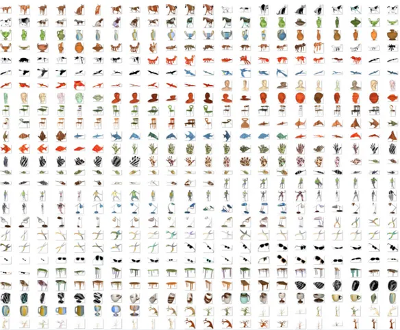
The dataset is made of 572 watertight mesh models, see Figure 1, grouped in 16 geometric classes of 32 or 36 instances. Each geometric class represents a type of ge-ometric shape (e.g., humans, birds, trees, etc). Besides the geometric classification, models are also classified in 12 texture classes. Each texture class is characterized by a precise pattern (e.g., marble, wood, mimetic, etc). The collection is built on top of a set of null models, that is, base meshes endowed with two or three different textures. All the other elements in the dataset come as the result of applying a shape transformation to one of the null shapes, so that a geometric and a texture deformation are randomly combined case by case.
The geometric deformations include the addition of Gaussian noise, mesh re-sampling, shape bending, shape stretching and other non-isometric transforma-tions that do not necessarily preserve the metric prop-erties of shapes (e.g. the Riemannian metric).
As for texture deformations, they include topolog-ical changing and scaling of texture patterns, as well as affine transformations in the RGB colour channels, resulting in, e.g., lighting and darkening effects, or in a sort of pattern blending. While the topological texture deformation has been applied manually, affine transfor-mations admit an analytic formulation. A numerical pa-rameter allows to tune each analytic formulation, thus making possible to automatically generate a family of texture deformations. In our dataset, texture transfor-mations are grouped in five families, each family being the result of three different parameter values.
Figure 2 illustrates some geometric and texture de-formations in action. The added value in working with a dataset built in this way is that particular weaknesses and strengths of algorithms can be better detected and analysed. Indeed, methods can be evaluated in specific tasks, for example retrieval against (simulated) illumi-nation changing or degradation of texture pattern. This is actually part of the proposed comparative study, see Section 5.1.1 for more details.
Together with the dataset, a training set made of 96 models classified according to both geometry (16 classes) and texture (12 classes) has been made avail-able for methods requiring a parameter tuning phase.
3.2 The retrieval and classification tasks
In our analysis we distinguished two tasks: retrieval and classification. For each task, at most three runs for each method have been considered for evaluation, being the result of either different parameter settings or more
sub-Fig. 1 The collection of textured 3D models used in the comparative study.
(a) (b) (c) (d) (e)
(f ) (g) (h) (i) (l)
Fig. 2 Two base models (a, f ) together with some purely geometric (b − e) and purely texture (g − l) modifications.
stantial method variations.
Retrieval task. Each model is used as a query against the rest of the dataset, with the goal of retrieving the most relevant objects. For a given query, a retrieved object is considered highly relevant if the two models share both geometry and texture; marginally relevant if they share only geometry; not relevant otherwise. For this task, a dissimilarity 572 × 572 matrix was required,
each element (i, j) recording the dissimilarity value be-tween models i and j in the whole dataset.
Classification task. The goal is to assign each query to both its geometric and texture class. To this aim, a nearest neighbour (1-NN) classifier has been derived from the dissimilarity matrices used in the retrieval task. For each run, the output consists of two classifica-tion matrices, a 572 × 16 one for the geometric
classifi-cation and a 572 × 12 one for the texture classificlassifi-cation. In these matrices, the element (i, j) is set to 1 if i is classified in class j (that is, the nearest neighbour of model i belongs to class j), and 0 otherwise.
3.3 The evaluation measures
The following measures have been used to evaluate the retrieval and classification performances of each method. 3.3.1 Retrieval evaluation measures
3D retrieval evaluation has been carried out according to standard measures, namely precision-recall curves, mean average precision, Nearest Neighbour, First Tier, Second Tier, Normalized Discounted Cumulated Gain and Average Dynamic Recall [76].
Precision-recall curves and mean average precision. Precision and recall are common measures to evaluate information retrieval systems. Precision is the fraction of retrieved items that are relevant to the query. Recall is the fraction of the items relevant to the query that are successfully retrieved. Being A the set of relevant objects and B the set of retrieved object,
Precision = |A ∩ B|
|B| , Recall =
|A ∩ B|
|A| .
Note that the two values always range from 0 to 1. For a visual interpretation of these quantities it is useful to plot a curve in the reference frame recall vs. preci-sion. We can interpret the resul as follows: the larger the area below such a curve, the better the performance un-der examination. In particular, the precision-recall plot of an ideal retrieval system would result in a constant curve equal to 1. As a compact index of precision vs. recall, we consider the mean average precision (mAP), which is the portion of area under a precision recall-curve: from the above considerations, it follows that the maximum mAP value is equal to 1.
Nearest Neighbour, First Tier and Second Tier. These evaluation measures aim at checking the fraction of models in the query’s class also appearing within the top k retrievals. Here, k can be 1, the size of the query’s class, or the double size of the query’s class. Specifically, for a class with |C| members, k = 1 for the nearest neighbour (NN), k = |C| − 1 for the first tier (FT), and k = 2(|C| − 1) for the second tier (ST). Note that all these values necessarily range from 0 to 1.
Average dynamic recall. The idea is to measure how many of the items that should have appeared before or
at a given position in the result list actually have ap-peared. The average dynamic recall (ADR) at a given position averages this measure up to that position. Pre-cisely, for a given query let A be the set of highly rel-evant (HR) items, and let B be the set of marginally relevant (MR) items. Obviously A ⊆ B. The ADR is computed as: ADR = 1 |B| |B| X i=1 ri, where ri is defined as ri=
(|{HR items in the first i retrieved items}|
i , if i ≤ |A|;
|{MR items in the first i retrieved items}|
i , if i > |A|.
Normalized discounted cumulated gain. It is first conve-nient to introduce the discounted cumulated gain (DCG). Its definition is based on two assumptions. First, highly relevant items are more useful if appearing earlier in a search engine result list (have higher ranks); second, highly relevant items are more useful than marginally relevant items, which are in turn more useful than not relevant items. Precisely, the DCG at a position p is defined as: DCGp= rel1+ p X i=2 reli log2(i) ,
with relithe graded relevance of the result at position i. Obviously, the DCG is query-dependent. To overcome this problem, we normalize the DCG to get the normal-ized discounted cumulated gain (NDCG). This is done by sorting elements of a retrieval list by relevance, pro-ducing the maximum possible DCG till position p, also called ideal DCG (IDCG) till that position. For a query, the NDCG is computed as
NDCGp=
DCGp
IDCGp .
It follows that, for an ideal retrieval system, we would have NDCGp= 1 for all p.
3.3.2 Classification performance measures.
We also consider a set of performance measures for clas-sification, namely confusion matrix, sensitivity, speci-ficity and the Mattews correlation coefficient [19, 49]. Confusion matrix. Each classification performance can be associated with a confusion matrix CM , that is, a square matrix whose order is equal to the number of classes (according to either the geometric or the tex-ture classification) in the dataset. For a row i in CM ,
the element CM (i, i) gives the number of items which have been correctly classified as elements of class i; sim-ilarly, elements CM (i, j), with j 6= i, count items which have been misclassified, resulting as elements of class j rather then elements of class i. Thus, the classification matrix CM of an ideal classification system should be a diagonal matrix, such that the element CM (i, i) equals the number of items belonging to the class i.
Sensitivity, specificity and Matthews correlation coeffi-cient. These statistical measures are classical tools for the evaluation of classification performances. Sensitiv-ity (also called the true positive rate) measures the pro-portion of true positives which are correctly identified as such (e.g. the percentage of cats correctly classified as cats). Specificity (also known as true negative rate) measures the proportion of true negatives which are cor-rectly identified as such (e.g. the percentage of non-cats correctly classified as non-cats). A perfect predictor is 100% sensitive and 100% specific.
The Matthews correlation coefficient takes into ac-count true and false positives and negatives and is gen-erally regarded as a balanced measure which can be used even if the classes are of very different sizes. The MCC is in essence a correlation coefficient between the observed and predicted classifications; it returns a value between -1 and 1. A coefficient of 1 represents a per-fect classification, 0 no better than random classifica-tion and -1 indicates total disagreement between clas-sification and observation.
4 Description of the methods
Six methods for textured 3D shape retrieval and clas-sification have been implemented. In this section we describe them in detail, focusing also on their possible variations and the choice of the parameters adopted to implement the runs used in our comparative evaluation. 1. Histograms of Area Projection Transform and Colour
Data and Joint Histograms of MAPT and RGB data (runs GG1,GG2,GG3), Section 4.1. These runs are based on a multi-scale geometric description able to capture local and global symmetries coupled with histograms of the normalized RGB channels; 2. Spectral geometry based methods for textured 3D
shape retrieval (runs LBG1, LBG2, LBG3 and LBGtxt), Section 4.2. These runs combine an in-trinsic, spectral descriptor with the concatenated histogram of the RGB values;
3. Colour + Shape descriptors (runs Ve1, Ve2, Ve3), Section 4.3. These runs adopt combinations (with different weights) of the histogram of the RGB
val-ues with a geometric descriptors represented by the eigenvalues of the geodesic distance matrix; 4. Textured shape distribution, joint histograms and
persistence (runs Gi1, Gi2, Gi3), Section 4.4. These runs combine several geometric, colourimetric and hybrid descriptors: namely, the spherical harmonics descriptor, the shape distributions of the geodesic distances weighted with the colourimetric attributes and a persistence-based description based on the CIELab space;
5. Multiresolution Representation Local Binary Pat-tern Histograms (run TAS), Section 4.5. This run captures the geometric information through the com-bination of a multi-view approach with local binary patterns and combines it with the concatenated his-tograms of the CIELab colour channels;
6. PHOG: Photometric and geometric functions for textured shape retrieval (runs BCGS1, BCGS2, BCGS3), Section 4.6. These runs combine a shape descriptor based on geometric functions; a persistence-based descriptor built on a generalized notion of geodesic distance that combines geometric and colouri-metric information; a purely colouricolouri-metric descrip-tor based on the CIELab colour space.
4.1 Histograms of Area Projection Transform and Colour Data and Joint Histograms of MAPT and RGB data (runs GG1-3)
Computing the similarity between textured meshes is achieved according to two different approaches based on histograms of Multiscale Area Projection Transform (MAPT) [25]. MAPT originates from the Area Projec-tion Transform (APT), a spatial map that measures the likelihood of the 3D points inside the shape of be-ing centres of spherical or cylindrical symmetry. For a shape S represented by a surface mesh S, the APT is computed at a 3D point x for a radius of interest r: APT(x, S, r, σ) = Area(Tr−1(kσ(x) ⊂ Tr(S, n))), where Tr(S, n) is the surface parallel to S shifted along the inward normal vector n for a distance r, and kσ(x) is a sphere of radius σ centred in x. APT values at different radii are normalized to have a scale-invariant behaviour, creating the Multiscale APT (MAPT): MAPT(x, S, r) = APT(x, S, r, σ(r))4πr2 ,
with σ(r) = c · r for 0 < c < 1.
A discrete version of the MAPT function is imple-mented following [25]. Roughly, the map is estimated on a grid of voxels with side length s and for a set of
corresponding sampled radius values r1, ..., rt. This grid partitions the mesh’s bounding box, but only the voxels belonging to the inner region of the mesh are considered when creating the histogram.
Histograms of MAPT are very good global shape descriptors, performing state of the art results on the SHREC 2011 non-rigid watertight contest dataset [43]. For that retrieval task, the MAPT function was com-puted using 8 different scales (radius values) and the map values were quantized in 12 bins; finally the 8 his-tograms were concatenated creating an unique descrip-tor of length 96. The voxel size and the radius values were chosen differently for each model, proportionally to the cube root of the object volume, in order to have the same descriptor for scaled versions of the same ge-ometry. The value of c was always set to 0.5.
To deal with textured meshes, the MAPT approach has been modified in two different ways, so to exploit also the colour information.
4.1.1 Histograms of MAPT and Colour Data
MAPT histograms are computed with the same radii and sampling grid values as in [25]: the isotropic sam-pling grid is proportional to the cube root of the volume V of each model, that is, of side length s = √3
V /30), and the sampled radii are integer multiples of s (10 values from 2s to 11s). The radius σ is taken, as in the original paper, equal to ri/2 for all the sampled ri. Fur-thermore, for each mesh the histogram of colour com-ponents is computed. With this procedure each mesh is described by two histograms, the first one representing the geometric information and the second one repre-senting the texture information. The total dissimilarity between two shapes S1, S2is then assessed using a con-vex combination of the two histogram distances: D(S1, S2) = γ dgeo(S1, S2) + (1 − γ) dclr(S1, S2), (1) where 0 ≤ γ ≤ 1 , dgeo(S1, S2) is the normalized Jeffrey divergence between the two MAPT histograms of S1 and S2, and dclr(S1, S2) corresponds to the normalized χ2-distance of the two colour histograms. The choice of γ in (1) allows the user to decide the relevance of colour information in the retrieval process.
Results shown in Section 5 are obtained by applying two different pre-processing steps to the RGB values, both adopted to have a colour representation that is invariant to illumination changes.
The first method, resulting in run GG1, is a simple contrast stretching for each RGB channel, mapping the min-max range of each channel to [0, 1]. In this case the colour quantization is set to 4 bins for each normalized RGB channels and γ is set to 0.6.
The second model, corresponding to run GG2, is the greyworld representation [20] in which each RGB value is divided by its corresponding channel mean value: (Rg = R/Ravg, Gg = G/Gavg, Bg = B/Bavg). Here, γ = 0.6 and the 4 histogram bins are centred in the mean value and are linearly distributed within a range of [0, 2] for each greyworld RGB channel.
4.1.2 Joint Histograms of MAPT and greyworld RGB data
To get run GG3, a new descriptor has been designed by concatenating the original APT histogram with those obtained from the 3 components of the selected (nor-malized) colour space. For each voxel, the APT is evalu-ated at a certain radius; the procedure is then repeevalu-ated for all the radius values (r1, ..., rt), and the t histograms are finally linearized and concatenated. In the present paper, a sampling grid with side length s = √3
V /18 has been used for each model, together with 9 sampled radii that are integer multiples of s (t = 9 values from 2s to 10s). The APT target set has been divided into 8 bins. As for the colour components, the above grey-world RGB representation has been adopted, and each channel has been quantized in 4 bins in the range [0, 2]. The dissimilarity between two meshes is obtained with the normalized Jeffrey divergence [15] between the two corresponding linearized and concatenated sets of joint histograms.
4.2 Spectral geometry – based methods for textured 3D shape retrieval (runs LBG1-3, LBGtxt)
This method is build on the spectral geometry-based framework proposed in [37], suitably adapted for tex-tured 3D shape representation and retrieval.
The spectral geometry approach, which is based on the eigendecomposition of the Laplace-Beltrami opera-tor (LBO), provides a rich set of eigenbases invariant to isometric transformations. Also, these eigenbases serve as ingredients for two further steps: feature extraction, detailed in Section 4.2.1, and spatial sensitive shape comparison via intrinsic spatial pyramid matching [39], discussed in Section 4.2.2. The cotangent weight scheme [14] was used to discretize LBO. The eigenvalues λiand associated eigenfunctions ϕi can be computed by solv-ing the generalized problem
Cϕi= λiAϕi, i = 1, 2, . . . , m,
where A is a positive-definite diagonal area matrix and C is a sparse symmetric weight matrix. In the proposed implementation, m is set to 200.
4.2.1 Feature extraction
The first step consists in the computation of an infor-mative descriptor at each vertex of a triangle mesh rep-resenting a shape. The spectral graph wavelet signa-ture [40] is used to capsigna-ture geometry information and colour histogram to encode texture information. Geometry information. In general, any of the spectral descriptors with the eigenfunction-squared form reviewed in [41] can be considered in this framework for isomet-ric invariant representation. Here, the spectral graph wavelet signature (SGWS) is adopted as local descrip-tor. SGWS provides a general and flexible interpreta-tion for the analysis and design of spectral descriptors. For a vertex x of a triangle mesh, it is defined as SGWSt(x) =
m X
i=1
g(t, λi)ϕ2i(x).
In a bid to capture both global and local geometry, a multi-resolution shape descriptor is derived by set-ting g(t, λi) as a cubic spline wavelet generating kernel and considering the scaling function (see [40, Eq. (20)] for a precise formulation of g). This leads to the multi-scale descriptor defined as SGWS(x) = {SGWSt(x), t = 1, . . . , T }, with T the chosen resolution and SGWSt(x) the shape signature at the resolution level t. In the pro-posed implementation T is set to 2.
Texture information. Colour histograms (CH) are used to characterize texture information on the surface. Each channel is discretized into 5 bins.
4.2.2 Shape comparison via intrinsic spatial pyramid matching
To incorporate the spatial information, the Intrinsic Spatial Pyramid Matching (ISPM) [39] is considered. ISPM can provably imitate the popular spatial pyra-mid matching (SPM) [35] to partition a mesh in a con-sistent and easy way. Then, Bag-of-Feature (BoF) and Locality-constrained Linear Coding (LLC) [78] can be used to characterize the partitioned regions.
The isocontours of the second eigenfunction (Fig-ure 3) are considered to partition the shape into R re-gions, with R = 2l−1 for the partition at a resolu-tion level l. Indeed, the second eigenfuncresolu-tion is the smoothest mapping from the manifold to the real line, making this intrinsic partition quite stable. Thus, the shape description is given by the concatenation of R sub-histograms of SGWS and CH along eigenfunction values in the real line. To consider the two-sign pos-sibilities in the concatenation, the histogram order is
inverted, and the scheme with the minimum cost is con-sidered as a better matching. Therefore, the descriptive power of SGWS and CH is enhanced by incorporating this spatial information.
Fig. 3 The isocontours of the second eigenfunction.
Given a SGWS+CH descriptor densely computed on each vertex on a mesh, quantization via the code-book model approach is adopted to obtain a compact histogram shape representation. The classical k-means method is used to learn a dictionary Q = {q1, . . . , qK}, where words are obtained as the K centroids of the k-means clusters. In the proposed implementation, K = 100. In order to assign the descriptor to a word in the vocabulary, approximated LLC is performed for fast en-coding, then max-pooling is applied to each region. Fi-nally, ISPM induced histograms for shape representa-tion are derived.
The dissimilarity between two shapes is given by L2 distance between the associated ISPM induced his-tograms. Geometry and texture information are han-dled separately, and the final dissimilarity score is a combination of the geometric and the texture distance.
4.2.3 The runs
The proposed approach has been implemented to derive three different runs for the retrieval task:
– LBG1 represents LCC strategy with partition level l = 1 for geometric information;
– LBG2 represents LCC strategy with partition level l = 3 for geometric information;
– LBG3 is a weighted combination of geometric and texture information, namely LCC strategy with par-tition level 3 for SGWS and parpar-tition level l = 5 for colour histograms, with coefficients 0.8 and 0.2, re-spectively.
For the classification task, two nearest neighbour classifiers are derived, a geometric one from LBG2 and a texture one from the texture contribution of LBG3. In what follows, the latter is referred to as LBGtxt.
4.3 Colour + Shape descriptors (runs Ve1-3)
This method is a modification of the “3D Shape + colour” descriptor proposed in [9]. To describe a tex-tured 3D shape S represented by a surface mesh S, two main steps are considered:
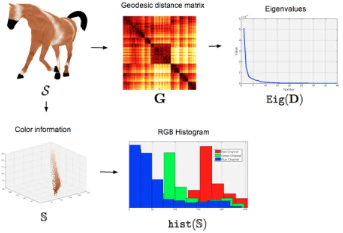
1. Let G be a n × n geodesic distance matrix, where n is the number of vertices in S and the element G(i, j) denotes the geodesic distance from the ver-tex i to verver-tex j on S. Building on G, the centralised geodesic matrix [50] is defined as D = G − 1nG − G1n+1nG1n, where 1ndenotes a n×n matrix hav-ing each component equal to 1/n. Followhav-ing [68], a spectral representation of the geodesic distance is finally adopted as shape descriptor, that is, a vector of eigenvalues Eig(D) = (λ1(D), . . . , λn(D)), where λi(D) is the ith largest eigenvalue. As in [9], the first 40 eigenvalues are used as shape descriptor. The vectors of eigenvalues Eig(D1), Eig(D2) associated with two shapes S1, S2 are compared through the mean normalized Manhattan distance, i.e.,
dgeo(S1, S2)) = 40 X k=1 2|λk(D1) − λk(D2)| λk(D1) + λk(D2) .
2. To incorporate texture information in the shape de-scriptor, the RGB colour histograms are considered as in [9]. Accordingly, the distance dclr(S1, S2)) be-tween the texture shape descriptors associated with S1, S2is given by the Earth mover’s distance (EMD) between the corresponding RGB colour histograms. For two histograms p and q, the EMD measures the minimum work that is required to move the region lying under p to that under q. Mathematically, it has been defined as the total flow that minimizes the transport from p to q. We refer keen readers to [63] for a comprehensive review of EMD formu-lation, and to [58] for an application to shape re-trieval. To concretely evaluate EMD, the fast im-plementation introduced by [56] has been used with a thresholded ground distance.
Last, the final distance between S1and S2 is defined as follows:
D(S1, S2) = (dgeo(S1, S2))p+ (dclr(S1, S2))1−p, where p is a parameter to control the trade-off between colour and shape information. In the experiments, p = 0.75 (run Ve1), p = 0.85 (run Ve2), and p = 0.95 (run Ve3), following the paradigm that geometric shape prop-erties should be more important than colourimetric ones in the way humans interpret similarity between shapes. An illustration of the proposed description for a tex-tured shape is given in Fig. 4.
Fig. 4 Proposed method includes a shape descriptor from the geodesic distance matrix and a colour descriptor from the histogram representation of RGB colour information. Details are included in section 4.3
4.4 Textured shape distribution, joint histograms and persistence (runs Gi1-3)
The CIELab colour space well represents how human eyes perceive colours. Indeed, uniform changes of co-ordinates in the CIELab space correspond to uniform changes in the colour perceived by the human eye. This does not happen with some other colour spaces, for ex-ample the RGB space. In the CIELab colour space, tones and colours are held separately: the L channel is used to specify the luminosity or the black and white tones, whereas the a channel specifies the colour as ei-ther a green or a magenta hue and the b channel spec-ifies the colour as either a blue or a yellow hue. Run Gi1. The Textured Shape Distribution (TSD) de-scriptor is a colour-aware variant on the classical Shape Distributions (SD) descriptor [53]. Indeed, TSD con-sists of the distribution of colour-aware geodesic dis-tances, which are computed between a number of sam-ple points scattered over the surface mesh representing the 3D model.
The surface mesh is embedded in the 3-dimensional CIELab colour space, so that each vertex has (L,a,b) co-ordinates. Then, in order to get colour-aware geodesic distances, a metric has to be defined in the embed-ding space. To this end, the length of an edge is de-fined as the distance between its endpoints, namely, the CIE94 distance defined for CIELab coordinates [18]. This distance is used here instead of a classical Eu-clidean distance as it was specifically defined for the CIELab space, and employs specific weights to respect perceptual uniformity [18]. The colour-aware geodesic distances are computed in the embedding space with
the metric induced by the CIE94 distance. The dis-tances are computed between pairs of points sampled over the surface mesh. A set of 1024 points was sampled in the current implementation, following a farthest-point criterion. The Dijkstra algorithm was used to compute colourimetric geodesic distances between pairs of sam-ples.
The final descriptor encodes the distribution of these distances. In the current implementation, the distribu-tion was discretized using a histogram of 64 bins. His-tograms were compared using the L2 norm. Therefore, the distance between two models is the distance be-tween their descriptors, namely the L2 norm between the corresponding histograms. TSD encodes the distri-bution of colour distances, yet it also takes into account the connectivity of the underlying model, as distances are computed by walking on the surface model. In this sense, TSD can be considered as a hybrid descriptor, taking into account both colourimetric and geometric information.
Run Gi2. Though TSD retains some information about the shape of 3D models, in terms of the connectivity of the mesh representing the object, it still loses most of the geometric information about the object, as it does not take into account the length of the edges in the Euclidean space. This geometric information can be re-covered by using a joint distribution, which takes into account both colourimetric geodesic distances and clas-sical geodesic distances computed on the surface em-bedded in the Euclidean space. In this run, the joint distribution has been discretized by computing a 16×16 bi-dimensional joint histogram (JH) for each 3D model. The L2-norm is used for comparison. The distance ma-trix is the sum of the distance mama-trix obtained using the TSD descriptor and the distance matrix obtained using the JH descriptor.
Run Gi3. In [5] the authors proposed a signature which combines geometric, colourimetric, and hybrid descrip-tors. In line with this idea, Run Gi3 combines TSD with a geometric descriptor, namely the popular Spherical Harmonic (SD) descriptor [29], and a colourimetric de-scriptor, namely the persistence-based descriptor of the PHOG signature in [5], using the CIELab colour space coordinates. The distance matrix corresponding to this run is the sum of the three distance matrices obtained using the TSD descriptor, the SH descriptor, and the persistence-based descriptor of PHOG, respectively.
4.5 Multi-resolution Representation Local Binary Pattern Histograms (run TAS)
The Multi-resolution Representation Local Binary Pat-tern Histograms (MRLBPH) is proposed here as a novel 3D model feature that captures textured features of rendered images from 3D models by analysing multi-resolution representations using Local Binary Pattern (LBP) [52].
Figure 5 illustrates the generation of MRLBPH. A 3D model is normalized via Point SVD [74] to be con-tained in a unit geodesic sphere. From each vertex of the sphere, depth and colour buffer images with 256 × 256 resolution are rendered; a total of 38 viewpoints are de-fined. A depth channel and each CIELab colour channel are then processed as detailed in what follows.
To obtain multi-resolution representations, a Gaus-sian filter is applied to an image with varying standard deviation parameters. The standard deviation param-eter σl at level l is evaluated by using the following equation involving the left factorial of l:
σl= σ0+ α·!l, l = 0, . . . , Λ
where σ0 is the initial value of the standard deviation parameter, and α is the incremental parameter. This equation has been derived from the optimal standard deviation parameters obtained through preliminary ex-periments. In the proposed implementation, σ0 = 0.8 and α = 0.6, while the number of levels Λ is set to 4.
For each scale image, a LBP histogram is evaluated. To incorporate spatial location information, the image is partitioned into 2 × 2 blocks and the LBP histogram at each block is computed. The LBP histogram of each scale image is obtained by concatenating the histograms of these blocks. Let gc denote the image value at arbi-trary pixel (u, v), and let g1, . . . , g8be the image values of each of the eight neighbourhood pixels. The LBP value is then calculated as
LBP(u, v) = 8 X
i=1
s(t, gi− gc) · 2i−1,
where s(t, g) is a threshold function defined as 0 if g < t and 1 otherwise. In the proposed implementation, the threshold value t is set to 0, and the LBP values are quantized into 64 bins.
An MRLBP histogram is generated by merging the histograms of scale images through the selection of the maximum value of each histogram bin. Let h(l)i be the ith LBP histogram element of a scale image at level l. The ith MRLBP histogram element hi is defined as hi = max
l h
(l)
L a b Max 3D model Depth images LBP histograms Multiresolution Representations MRLBP histogram ... ... ... ... Lab images
Fig. 5 Overview of our Multiresolution Representation Local Binary Pattern Histograms (MRLBPH)
The MRLBP histogram is finally normalized using the L1 norm.
The feature vector associated with a 3D model is obtained by calculating the MRLBP histogram of the depth and CIELab channel for each viewpoint.
To compare two shapes S1 and S2, the Hungarian method [34] is applied to all dissimilarities between the associated MRLBP histograms. In evaluating the final dissimilarity score, the histograms of the depth and CIELab channels are combined by calculating the weighted sum of each dissimilarity. Let dd, dL, da, and db denote the dissimilarity of each channel, and let wd, wL, wa, and wb be the weight of each channel. The dissimilarity D(S1, S2) is defined as the dissimilarity between the corresponding MRLBP histograms: D(S1, S2) = wddd(S1, S2) + wLdL(S1, S2)
+wada(S1, S2) + wbdb(S1, S2).
In this implementation, wdis set to 0.61, wLto 0.13, wa to 0.13, and wb to 0.13. For the dissimilarity between two histograms, the Jeffrey divergence is used [15].
4.6 PHOG: Photometric and geometric functions for textured shape retrieval (runs BCGS1-3)
The combination of colourimetric properties and ge-ometric properties represented in terms of scalar and multi-variate functions has been explored in PHOG [5], a shape signature consisting of three parts:
– A colourimetric descriptor. CIELab colour coordi-nates (normalized L, a, b channels) are seen as ei-ther scalar or multi-variate functions defined over the shape. The CIELab colour space is considered due the perceptual uniformity of this colour repre-sentation;
– A hybrid descriptor. Shape and texture are jointly analysed by opportunely weighting the colourimet-ric information (L, a, b channels) with respect to the underlying geometry and topology;
– A geometric description relying on a set of functions representing as many geometric shape properties.
Functions are first clustered; then, a representative function is chosen for each cluster. The goal here is to select functions that are mutually independent, thus complementing each other via the geometric information they carry with them.
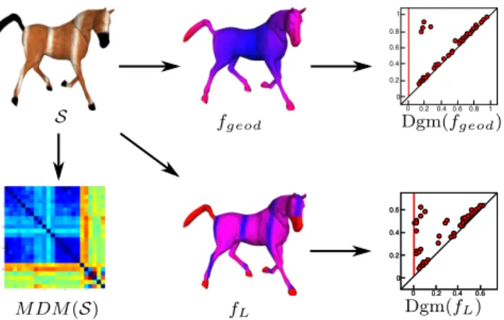
Figure 6 shows a pictorial representation for the gener-ation of a PHOG signature.
Run BCGS1. Following the PHOG original setting, the colourimetric description is included in the persis-tence framework. Indeed, the a, b coordinates are used to jointly define a bivariate function over a given shape, whereas L is used as a scalar function. In this way, colour and intensity are treated separately. Precisely, for a shape S represented by a triangle mesh S, the two functions fL: S → R and fa,b: S → R2are considered, the former taking each point x ∈ S to the L-channel value at x, the latter to the pair given by the a- and the b-channel values at x, respectively. The values of fLand fa,bare then normalized to range in the interval [0,1]. Last, S is associated with the 0th persistence dia-gram Dgm(fL) and the 0th persistence space Spc(fa,b): these descriptors encode the evolution of the connectiv-ity in the sublevel sets of fL and fa,b in terms of birth and death (i.e. merging) of connected components, see [5] for more details.
The hybrid description comes from a geodesic dis-tance fgeod : S → R defined in a higher dimensional embedding space, similarly to the approach proposed in [31, 33], and used as a real-valued function in the persistence framework to associate S with the persis-tence diagram Dgm(fgeod). The definition of the joint geometric and colourimetric integral geodesic distance is straightforward and implemented through the Dijk-stra’s algorithm, which is based on edge length.
The geometric description is based on the DBSCAN clustering technique [17]. Once a set of functions {fi : S → R} (from an original set of 70 geometric func-tions, see [5] for the complete list) is selected, a matrix M DM (S) with entries M DM (i, j) := 1 −Area(S)1 X t∈S < ∇ tf i k∇tf ik , ∇ tf j k∇tf jk >
is used to store the distances between all the possible couple of functions, with ∇tf
i, ∇tfj representing the gradient of fi and fj over the triangle t of the mesh S. To assess the similarity between two shapes S1 and S2, the corresponding colourimetric, hybrid and geo-metric descriptions are compared. In particular, the colourimetric distance dclr(S1, S2) is the normalized sum of the Hausdorff distance between the 0th persistence diagrams of fL and that between the 0th persistence
0 0.2 0.4 0.6 0 0.20.40.60.8 1 0.8 1 0 0.2 0.4 0.6 0 0.2 0.4 0.6 0 0.2 0.4 0.6 0 0.2 0.4 0.6 S fgeod Dgm(fgeod) M DM(S) fL Dgm(fL)
Fig. 6 Generating a PHOG signature. First row: A shape S (left), the function fgeod(center) and the corresponding
per-sistence diagram Dgm(fgeod). Second row: the mutual
dis-tance matrix M DM (S), the function fLand the
correspond-ing persistence diagram Dgm(fL).
spaces of fa,b; the hybrid distance dhbd(S1, S2) is the Hausdorff distance between the corresponding persis-tence diagrams of fgeod; the geometric distance dgeo(S1, S2) is computed as the Manhattan distance between the matrices M DM (S1) and M DM (S2). The final dissim-ilarity score between S1 and S2 is the normalized sum dclr(S1, S2) + dhbd(S1, S2) + dgeo(S1, S2).
Variations. Several variations of the PHOG framework are possible, for instance exploring the use of different distances between feature vectors or dealing with vari-ations of the three (colourimetric, hybrid, geometric) shape descriptions. For the current implementation the following changes have been proposed:
– run BCGS2. The original hybrid description is re-placed by a histogram-based representation of the geodesic distance. While getting rid of the addi-tional geometric contribution provided by persis-tence, the hybrid perspective is maintained as the considered geodesic distance takes into account both geometric and texture information.
– run BCGS3. The stability properties of persistence diagrams and spaces imply robustness against small variations in the L, a, b values. This also holds when colour perturbations are widely spread over the sur-face model, as in the case of slight illumination changes. On the other hand, colour histograms behave well against localized colourimetric noise, even if charac-terized by large variations in the L, a, b values. In-deed, in this case colour distribution is not altered greatly. In this view, the idea is to replace the hy-brid contribution with CIELab colour histograms, so to improve the robustness properties of the the persistence-based description. Histograms are
ob-tained as the concatenation of the L, a, b colour chan-nels.
In Runs BCGS2-3, histograms are compared through the Earth Mover’s distance (EMD). The DBSCAN clus-tering technique for selecting representative geometric functions is replaced by the one used in [8], which is based on the replicator dynamics technique [55]. The modified geometric descriptors are compared via the EMD as well, after converting the M DM matrices into feature vectors.
4.7 Taxonomy of the methods
The methods detailed above can be considered as repre-sentatives of the variety of 3D shape retrieval and clas-sification techniques overviewed in Section 2. Indeed, they range from local feature vector descriptions coded as histograms of geometric and/or colour properties, to spectral and topological based descriptions, including also a spatial pyramid matching framework. In what follows, we group the properties of these methods on the basis of the key characteristics they exhibit, e.g., the geometric and colourimetric structure they capture, at which scale level the shape description is formalized, or which colour space has been chosen for texture anal-ysis. These characteristics are briefly described in the following and summarized in Table 1.
Intrinsic vs. extrinsic. Studying the geometric shape of a 3D model relies on the definition of a suitable metric between its points. Among the possible options, two particular choices appear quite natural.
The first one is to consider the Euclidean distance, which in turn reflects the extrinsic geometry of a shape. Extrinsic shape properties are related to how the shape is laid out in an Euclidean space, and are therefore invariant to rigid transformations, namely rotations, translations an reflections.
A second choice is to measure the geodesic distance between points, that is, to consider the intrinsic geom-etry of a shape. Intrinsic shape properties are invariant to those transformations preserving the intrinsic metric, including rigid shape deformations but also non-rigid ones such as shape bendings.
Methods associated with runs GG(1-3), TAS and Gi3 are examples of extrinsic approaches; spectral meth-ods (runs LBG(1-3)) and those based on geodesic dis-tances (runs Ve(1-3) and Gi(1-2)) well represent in-trinsic approaches. The PHOG method (runs BCGS(1-3)) can be seen as a “mostly” intrinsic approach, be-ing based on a collection of geometric functions which
prevalently describe intrinsic shape properties.
Global vs. multi-scale. Shape descriptors generally en-code information about local or global shape properties. Local properties reflect the structure of a shape in the vicinity of a point of interest, and are usually unaffected by the geometry or the topology outside that neigh-bourhood. Global properties, on the other hand, cap-ture information about the whole struccap-ture of a shape. Another option is to deal with shape properties at different scales, thus providing a unifying interpretation of local and global shape description. Such an approach is usually referred to as multi-scale.
The methods presented in this contribution can be classified as global and multi-scale ones, both for geo-metric and texture information, see Table 1 for details. RGB vs. non-RGB. The more natural colour space to be used in the analysis of colourimetric shape prop-erties appears to be the RGB one. This was actually the choice carried on by methods associated with runs LBGtxt and Ve(1-3). However, other options are pos-sible. For instance, runs GG(1-3) are based on normal-ized and averaged RGB channels, while methods related to runs TAS, BCGS(1-3), Gi(1-3) study colourimet-ric shape properties in the CIELab colour space. Feature vectors vs. topology. Once geometric and tex-ture shape properties have been analysed and captex-tured, they have to be properly represented through suitable shape descriptors. The most popular approach is to use feature vectors [73], and most of the methods im-plemented in this paper actually adopt this descrip-tion framework. Feature vectors generally encode shape properties expressed by functions defined on the shape, and are usually represented as histograms. While be-ing very efficient to compute, histograms might forget part of the structural information about the consid-ered shape property. To overcome this limitation, it is possible to consider the shape connectivity directly at the function level, see for instance shape distributions (runs Gi1 and Gi2). Alternatively, one can move to more informative histogram variations: bi-dimensional histograms, such as the geodesic distance matrix used in runs Ve(1-3) and the mutual distance matrix adopted in runs BCGS(1-3), or concatenated histograms ob-tained at different resolution levels, as in the case of runs GG(1-3), LBG(1-3,txt) and TAS.
A different way to preserve the structure of geo-metric information is provided by descriptors rooted in topology (runs BCGS(1-3) and Gi3). Indeed, they keep track of the spatial distribution of a considered shape property, and possibly encode the mutual relation
among shape parts of interest, that is, regions that are highly characterized by the considered property. The reader is referred to Table 1 for details about the ap-proaches adopted by methods under evaluation. Hybrid vs. combined. Finally, methods can be distin-guished by the way the geometric and texture informa-tion are merged together. Typically, this can be done either a priori or a posteriori. The first case results in a hybrid shape descriptor, as for runs GG3 and par-tially for runs BCGS(1-3) and Gi(1-3). In the second case, a pure geometric and a pure texture descriptor are obtained and compared separately, while the final dissimilar score is a weighted combination of the two distances.
5 Comparative analysis
The methods detailed in Section 4 have been evaluated through a comparative study presented in what follows. Each run has been processed in terms of the output specified in Section 3.2 and according to the evaluation measures described in Sections 3.3.1 and 3.3.2.
5.1 Retrieval performances.
Following [76], the retrieval performance of each run has been evaluated according to the following relevance scale: if a retrieved object shares both shape and tex-ture with the query, then it is highly relevant; if it shares only shape, it is considered marginally relevant; other-wise, it is not relevant. Note that, because of the multi-level relevance assessment of each query, most of the evaluation measures have been split up as well. Highly relevant evaluation measures relate to the highly rele-vant items only, while relerele-vant evaluation measures are based on all the relevant items (highly relevant items + marginally relevant items).
5.1.1 Highly relevant evaluation.
In the highly relevant scenario, the main goal is to eval-uate the performance of algorithms when models vary by both geometric shape and texture.
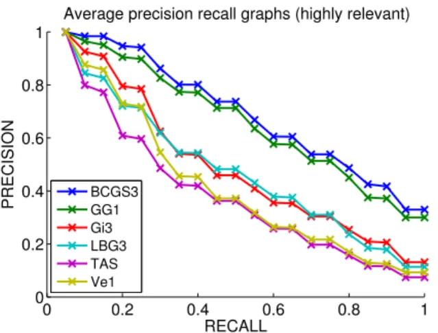
Figure 7 shows the performances of the six methods in terms of the average precision-recall curve, which is obtained as the average of the precision-recall curves computed over all the queries. To ease results visual-ization, the plot in Figure 7 includes only the best run for each method, that is, runs with the highest mean av-erage precision (mAP) score. We remind that, for ideal retrieval systems, the mAP score equals to 1.
0 0.2 0.4 0.6 0.8 1 0 0.2 0.4 0.6 0.8 1
Average precision recall graphs (highly relevant)
RECALL PRECISION BCGS3GG1 Gi3 LBG3 TAS Ve1
Fig. 7 Highly relevant precision-recall curves for the best run of each method.
The runs of Figure 7 have been analysed also in terms of the weighted average mAP score computed over the 48 classes that represent the highly relevant scenario, where weights are determined by the size of the classes, see the second column of Table 2. Moreover, we considered also the percentage of classes whose mAP score is larger that some threshold values, namely 0.40, 0.55, 0.70, 0.85, see columns (3-6) in Table 2.
Table 2 Highly relevant analysis for the runs in Figure 7: weighted average mAP score (first column), and how many of the 48 highly relevant classes have a mAP score exceeding values 0.40, 0.55, 0.70, 0.85 ((third - last column, respectively; results are reported in percentage points). The best two re-sults are in gold and silver text, respectively.
Runs mAP >(%)0.40 >(%)0.55 >(%)0.70 >(%)0.85 BCGS3 0.7225 100.00 79.17 52.08 27.08 GG1 0.6980 100.00 81.25 50.00 18.75 Gi3 0.5365 79.17 39.58 18.75 4.17 LBG3 0.5256 77.08 33.33 10.42 2.08 TAS 0.4380 64.58 12.50 2.08 0.00 Ve1 0.4671 68.75 29.17 4.17 0.00
To further analyse retrieval performances against texture deformations, we restrict the mAP analysis to each specific class of colourimetric transformations de-scribed in Section 3. More precisely, we first let the algorithms run exclusively on set of null models. Then, we add only those elements that come as a result of one of the five texture transformations used to generate the entire dataset. Note that, according to the procedure used to create the benchmark, each texture deforma-tion is always applied together with a geometric one, hence it still makes sense to apply the highly relevant
paradigm along the evaluation process. Table 3 sum-marizes the results.
Looking at how the performances degrade across the different families of transformations, it can be noted that all methods appear to be not too sensitive against transformations of type 2, while the worst results are distributed among transformations of type 1 (runs Gi3, LBG3, TAS and Ve2), and 3 (runs BCGS3 and GG1).
Table 4 reports the best highly relevant performances in terms of Nearest Neighbour, First Tier and Second Tier evaluation measures. Additionally, the last column of Table 4 records the ADR measures. All the scores, which range from 0 (worst case) to 1 (ideal perfor-mance), are averaged over all the models in the dataset.
Table 4 Best NN, FT, ST and ADR values for each method. Numbers in parenthesis indicate the run achieving the corre-sponding value. For each evaluation measure, the best two results are in gold and silver text, respectively.
Runs NN FT ST ADR BCGS 0.967(3) 0.620(3) 0.760(3) 0.496(3) GG 0.930(3) 0.600(1) 0.740(1) 0.478(1) Gi 0.894(2) 0.455(3) 0.590(3) 0.383(3) LBG 0.686(3) 0.440(3) 0.592(3) 0.369(3) TAS 0.558 0.375 0.527 0.318 Ve 0.735(1) 0.396(1) 0.539(1) 0.342(1)
Finally, Figure 8 shows the best run of each method according to the NDCG measure as a function of the rank p. In the present evaluation, the NDCG values for all queries are averaged to obtain a measure of the average performance for each submitted run. Remind that, for an ideal run, it would be NDCG ≡ 1.
0 100 200 300 400 500 0.4 0.5 0.6 0.7 0.8 0.9 1
Normalized discounted cumulated gain (NDCG)
rank p
NDCG at rank p (average on all queries)
BCGS3 GG1 Gi3 LBG3 TAS Ve1
Fig. 8 Performances of the best runs w.r.t. the NDCG mea-sure (run GG1 is almost totally covered by runs Gi3, LBG3 and TAS).
The NDCG measure takes geometric retrieval per-formances into larger account than texture ones.
In-deed, geometric shape similarity is involved in the def-inition of both relevant and highly relevant items. This means that runs characterized by moderate geometric retrieval performances will be more penalized than oth-ers (see also Section 5.1.2). This is the case of run GG1, which is indeed definitely tuned for the highly relevant rather then the relevant scenario.
Discussion. Trying to interpret the outcome of the highly relevant evaluation, we are led to the following consid-erations:
• The algorithm design associated with runs BCGS3 and Gi3 proposes a similar combination of geometric and texture information. Indeed, both methods rely on a hybrid shape description, in which texture con-tribution is in part based on a geometric–topological analysis of colourimetric properties and carried out in the CIELab colour space. In other words, a “struc-tured” analysis of the colour channels is paired with the choice of a colour space that better reflects, with respect to the RGB one, human colour perception. Moreover, the geometric–topological approach allows for keeping track of the underlying connectivity of 3D models, thus providing additional information about the spatial dis-tribution of colourimetric shape properties;
• Run GG1 represents a combined shape descrip-tor, whose texture contribution is based on considering a normalized version of the RGB colour space. Such a choice seems to imply a good robustness against texture affine transformations. Incidentally, it should be noted that, in spite of presenting only the best runs to ease readability and visualization of results, runs GG2 and GG3, which are based on the greyworld RGB chan-nels normalization, exhibit results which are compara-ble with those of run GG1;
• As for runs LBG and Ve, texture description is accomplished through standard histograms of RGB colour channels, although runs LBG incorporate some additional information as the result of considering a multi-resolution approach applied to shape sub-parts. However, it seems that dealing with colourimetric in-formation in other colour spaces, such as the CIELab one or variations of the RGB colour space, allows for a representation of colour that is more robust to the texture deformations proposed in this benchmark. 5.1.2 Relevant evaluation.
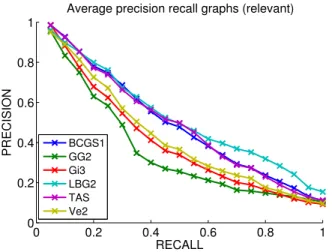
In this Section we analyse the performances of methods with respect to their capability of retrieving relevant items; in this case shape (dis)similarity depends only on geometric shape properties. In analogy to Section 5.1.1, Figure 9 shows the best runs for all methods in terms of
0 0.2 0.4 0.6 0.8 1 0 0.2 0.4 0.6 0.8 1
Average precision recall graphs (relevant)
RECALL PRECISION BCGS1GG2 Gi3 LBG2 TAS Ve2
Fig. 9 Relevant precison-recall curves for the best run of each method.
the average precision-recall curve. Table 5 reports the mAP scores of those runs, which are now averaged over the 16 geometric classes composing the dataset. Also in this case, we report for how many classes the mAP score exceeds values 0.40, 0.55, 0.70, 0.85.
Table 5 Relevant analysis for the runs in Figure 9: weighted average mAP score (first column), and how many of the 16 relevant classes have a mAP score exceeding values 0.40, 0.55, 0.70, 0.85 (third - last column, respectively; results are re-ported in percentage points). The best two results are in
gold and silver text, respectively.
Run mAP > .40 > .55 > .70 > .85 (%) (%) (%) (%) BCGS1 0.5181 81.25 37.50 6.25 0.00 GG2 0.3811 37.50 6.25 0.00 0.00 Gi3 0.4266 56.25 12.50 0.00 0.00 LBG2 0.5480 81.25 43.75 18.75 0.00 TAS 0.5158 81.25 37.50 12.50 0.00 Ve2 0.4479 56.25 25.00 12.50 0.00
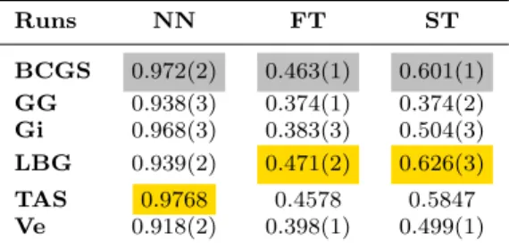
Table 6 reports the best relevant retrieval perfor-mances according to the Nearest Neighbour, First Tier and Second Tier evaluation measures. All scores are av-eraged over all the models in the dataset.
Discussion. Apart from the nearest neighbour scores (Table 6, first column), it seems that the overall rele-vant performance is still not ideal here. This is actu-ally not surprising, since most of methods considered for evaluation have been specifically tuned for dealing with both texture and geometric shape modifications. Nevertheless, the relevant evaluation can be used as a lever for further comments about the benchmark and the considered methods.
Table 6 Best NN, FT and ST values of each method. Num-bers in parenthesis indicate the run achieving the correspond-ing value. For each evaluation measure, the best two results are in gold and silver text, respectively.
Runs NN FT ST BCGS 0.972(2) 0.463(1) 0.601(1) GG 0.938(3) 0.374(1) 0.374(2) Gi 0.968(3) 0.383(3) 0.504(3) LBG 0.939(2) 0.471(2) 0.626(3) TAS 0.9768 0.4578 0.5847 Ve 0.918(2) 0.398(1) 0.499(1)
As an overall comment, it is worth mentioning that a large part of geometric shape modifications are not metric-preserving. Indeed, the geometric deformations used to create the benchmark alter both the extrinsic and the intrinsic properties of shapes. This suggests the need for the development of more general techniques for 3D shape analysis and comparison. This is actually one of the most recent trends in the field, see e.g. [60, 59].
More in detail, we observe that:
• The good performance of run LBG2 relies on two main motivations. First, this run is completely deter-mined by a geometric contribution, and therefore it is not affected by any other, possibly misleading, in-formation about texture shape properties. Second, the method represented by run LBG2 is spectral-based, and therefore is able to capture intrinsic shape prop-erties. As a consequence, it is invariant to rigid shape transformations, as well as some non-rigid deformations such as pose variations and bendings, which are all present in the dataset. Finally, differently from runs Gi3 and Ve2, whose geometric contribution is intrin-sic as well, the descriptive power of the spectral-based approach is improved by additional spatial information provided by the intrinsic spatial pyramid matching (see Section 4.2 for details);
• A similar reasoning about the invariance under rigid and non-rigid deformations also holds for run BCGS1, whose associated method can be considered as “mostly” intrinsic. Indeed, the geometric contribution relies in this case on a collection of descriptors which are mainly intrinsic, considering either spectral-based functions or geodesic distances or Gaussian curvature;
• The relatively good performance of run TAS can be explained by the fact that it mixes an extrinsic ap-proach with a “view-based” strategy that is widely ac-knowledged as the most powerful and practical approach for rigid 3D shape retrieval [67]. Even when a 3D model is articulated, non-uniformly deformed or partially oc-cluded, the number of views (38, actually) used in this
implementation should limit the noisy effect possibly generated in the images captured around an object;
• Run GG2 mainly focuses on radial and spherical local symmetries. While the approach appears to be robust when the analysis is restricted to a single class of geometric transformations, in the most general case (i.e. the whole dataset) results are affected by a non optimal trade-off between geometric and colourimetric contribution. In this way, the relevant retrieval perfor-mance is partially conditioned by the inter-class texture variations.
5.2 Classification performances.
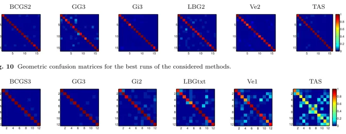
In the classification task, each run results in two classi-fication matrices, one for geometry and one for texture, which are derived from the 1-NN classifier associated with the dissimilarity matrices used for the retrieval task. Hence, for a classification matrix C, the element C(i, j) is set to 1 if model i is assigned to class j, mean-ing that j is the nearest neighbour of i, and 0 otherwise. Figures 10 and 11 represent the confusion matrices for the best runs of each method. For visual purposes, we have normalized the matrices with respect to the number of elements in each class, so that possible values range from 0 to 1.
Tables 7 and 8 provide a quantitative interpreta-tion of the visual informainterpreta-tion contained in the confu-sion matrices. Indeed, the true positive rate (TPR), the true negative rate (TNR) and the Matthews correlation coefficient (MCC) can be directly computed from the elements of a confusion matrix.
More precisely, given a confusion matrix CM and a class ¯ı, it is possible to derive the associated TPR, TNR and MCC as follows. It is first convenient to introduce the number of true positive TP, the number of false negative FN, the number of false positive FP and the number of true negative TN that are defined as TP = CM (¯ı.¯ı), FN = P
j6=¯ıCM (¯ı, j), FP = P
j6=¯ıCM (j, ¯ı),
TN =P
i,jCM (i, j) − (TP + TN + FP). Then, we get TPR, TNR and MCC by the relations
TPR = TP TP + FN, TNR = TN FP + TN, MCC = TP×TN−FP×FN p(TP+FP)(TP+FN)(TN +FP)(TN+FN). In Tables 7 and 8, the reported values are averaged over all the considered classes (16 geometric and 12 tex-tured ones).
Discussions. Dealing with 1-NN classifiers, the classifi-cation results resemble somehow the nearest neighbour performances registered in Tables 4 and 6. Note how-ever, that the dataset classifications considered in this
BCGS2 GG3 Gi3 LBG2 Ve2 TAS 5 10 15 5 10 15 5 10 15 5 10 15 5 10 15 5 10 15 5 10 15 5 10 15 5 10 15 5 10 15 5 10 15 5 10 15 0 0.2 0.4 0.6 0.8 1
Fig. 10 Geometric confusion matrices for the best runs of the considered methods.
BCGS3 GG3 Gi2 LBGtxt Ve1 TAS
2 4 6 8 10 12 2 4 6 8 10 12 2 4 6 8 10 12 2 4 6 8 10 12 2 4 6 8 10 12 2 4 6 8 10 12 2 4 6 8 10 12 2 4 6 8 10 12 2 4 6 8 10 12 2 4 6 8 10 12 2 4 6 8 10 12 2 4 6 8 10 12 0 0.2 0.4 0.6 0.8 1
Fig. 11 Texture confusion matrices for the best runs of the considered methods.
Table 7 Averaged geometric TPR, TNR and MCC for the best run of all considered methods. The best two results are in gold and silver text, respectively.
Run TPR TNR MCC BCGS2 0.9725 0.9988 0.9814 GG3 0.9371 0.9959 0.9341 Gi3 0.9685 0.9979 0.9668 LBG2 0.9388 0.9959 0.9355 TAS 0.9773 0.9985 0.9759 Ve2 0.9178 0.9945 0.9138
Table 8 Averaged texture TPR, TNR and MCC for the best run of all considered methods. The best two results are in
gold and silver text, respectively.
Run TPR TNR NCC BCGS3 0.9913 0.9992 0.9904 GG3 0.9860 0.9987 0.9847 Gi2 0.9161 0.9922 0.9093 LBGtxt 0.8811 0.9885 0.8714 TAS 0.5874 0.9621 0.5524 Ve1 0.8129 0.9820 0.7952
task are a purely geometric and a purely texture ones. In particular, the latter does not coincide with the clas-sification adopted in the highly relevant retrieval task, since geometric similarity is not involved. Also, results in Tables 7 and 8 are averaged on the dataset classes: this explains the slight discrepancy between the geo-metric TPR and the relevant NN measure that is aver-aged over all the elements in the dataset.
As shown by Figure 10, geometric confusion ma-trices reveal a good classification performance of the methods. Indeed, all matrices appear almost diagonal, meaning that almost all elements in the dataset should be correctly classified. This qualitative intuition is
con-firmed by the TPR scores reported in Table 7. Fur-thermore, TNR values are even higher, thus revealing that all methods are close to the optimal performance in detecting true negatives (e.g., “non-tables” correctly identified as such). As much in the same way, the MCC measure assigns scores very close to 1 for all methods.
Nevertheless, Figure 11 shows that, while the geo-metric classification of the considered runs are roughly comparable, in the texture scenario a sort of transition occurs, in such a way that three methods (BCGS3, GG3, Gi2) perform substantially better than the oth-ers. The numerical details in Table 8 highlight that the main differences are at the TPR and MCC level, reveal-ing that the confusion highlighted in Figure 11 is essen-tially in the localization of true positives (e.g., “tables” correctly identified as tables).
Finally, it is worth noting how, in the texture clas-sification task, best performances still come from those methods dealing with texture information in colour spaces which differ from the standard RGB one, that is, CIELab and the greyworld normalized RGB colour space.
6 Discussion and conclusions
In this paper, we have provided a detailed analysis and evaluation of state-of-the-art retrieval and classification algorithms dealing with an emerging type of content, namely textured 3D objects, which we believe deserve attention from the research community. The increasing availability of textured models in Computer Graphics, the advances in 3D shape acquisition technology which are able to acquire textured 3D shapes, the importance of colour features in 3D Shape Analysis applications together call for shape descriptors which take into con-sideration also colourimetric information.