HAL Id: hal-02343965
https://hal.archives-ouvertes.fr/hal-02343965
Submitted on 13 Nov 2019
HAL is a multi-disciplinary open access
archive for the deposit and dissemination of
sci-entific research documents, whether they are
pub-lished or not. The documents may come from
teaching and research institutions in France or
abroad, or from public or private research centers.
L’archive ouverte pluridisciplinaire HAL, est
destinée au dépôt et à la diffusion de documents
scientifiques de niveau recherche, publiés ou non,
émanant des établissements d’enseignement et de
recherche français ou étrangers, des laboratoires
publics ou privés.
Attribute profiles for satellite image time series
Caglayan Tuna, François Merciol, Sébastien Lefèvre
To cite this version:
Caglayan Tuna, François Merciol, Sébastien Lefèvre. Attribute profiles for satellite image time series.
IEEE International Geosciences and Remote Sensing Symposium (IGARSS), 2019, Yokohama, Japan.
�hal-02343965�
ATTRIBUTE PROFILES FOR SATELLITE IMAGE TIME SERIES
C
¸ aglayan Tuna, Franc¸ois Merciol, S´ebastien Lef`evre
IRISA - Universit´e Bretagne Sud, 56000 Vannes, France
{caglayan.tuna, francois.merciol, sebastien.lefevre}@irisa.fr
ABSTRACT
Morphological attribute profiles have been one of the most effective image features for spatial-spectral classification of remote sensing images during the last decade. The motiva-tion of this paper is to extend attribute profiles to satellite im-age time series, i.e. taking into account the temporal infor-mation. We introduce different approaches and report their performances for land cover mapping. Experiments are con-ducted on a Sentinel-2 dataset considering well-established supervised classification methods that are Random Forest and Support Vector Machines.
Index Terms— Attribute profiles, Satellite Image Time Series, Multiscale representation, Land cover mapping
1. INTRODUCTION
Analysis of Satellite Image Time Series (SITS) has gathered a growing interest due to the availability of high temporal frequency Earth Observation (EO) data provided by the new satellite missions (e.g. Sentinel). Therefore, analyzing EO time series is one of the significant trends in the remote sens-ing community. SITS have been used in many land use-land cover applications, land cover mapping being specifically a critical task [1]. Recently, using spatial features proved to be more efficient for classification purposes [2].
After the successful introduction of morphological pro-files [3] almost two decades ago, a significant progress was made ten years later with the more generic attribute profiles [4]. These profiles are made from successive applications of attribute filters, i.e. filters that operate on connected compo-nents of the level sets and that rely on some given attributes characterizing the image content (size, spectral or shape infor-mation). One of the reasons for the popularity of this frame-work is the efficient implementation that is achieved through the multiscale representation of an image, using morpholog-ical hierarchies (or trees) [5]. Indeed, processing nodes of a tree is much more efficient than dealing with the raw data. Each pixel of the image is then described by its so-called at-tribute profile, before a supervised or unsupervised classifi-cation is finally applied. The reader is referred to [6] for a
The authors wish to thank Centre National d’ ´Etudes Spatiales (CNES) and Collecte Localisation Satellites (CLS) for funding.
recent survey. Nevertheless, to the best of the authors’ knowl-edge, the application of such a framework to SITS remains particularly challenging. Thus, we explore in this paper var-ious strategies to do so, and conduct an experimental com-parison of these options. The rest of the paper is organized as follows. Section 2 provides mathematical background for morphological attribute profiles. In Section 3, we introduce several strategies to build such profiles on SITS. Experimen-tal results are reported in Section 4. Last, Section 5 concludes this paper with some future work hints.
2. MORPHOLOGICAL ATTRIBUTE PROFILES
Let I : Ω → V be a gray scale image with pixels defined on the spatial domain Ω ∈ N2and taking values in the finite
set V ∈ Z. An AP is obtained by filtering the image I with attribute operators using a predicate with increasing thresh-old values AP (I) = (IφλL, IφλL−1, ..., I, ..., IγλL−1, IγλL)
where φ and γ are thickening and thinning operators based on L ordered λ thresholds respectively. This attribute is cal-culated from the nodes, and examples include area, standard deviation, moment of inertia, etc [4]. AP can be efficiently computed through tree analysis, with min and max-tree used for thickening and thinning respectively. AP provides feature extraction in the spatial domain from images and gives useful results especially for classification.
AP relies on filtering through tree representations accord-ing to attributes in nodes. Filteraccord-ing simply consists in cuttaccord-ing the tree according to some predefined criteria, i.e. attribute thresholding. Filtering is straightforward in case of increasing attributes (whose value increase from leaves to root), while several strategies exist in case of non-increasing attributes [4] . We focus on two of the most common attributes: area, which is measured as the amount of pixels in a node, and moment of inertia that models the elongation of the node. While the former is increasing, the latter is not, and we consider here only the max-rule for the sake of simplicity.
3. TREES FOR SITS
The structure of a tree depends on a underlying hierarchy rule. In [5], two kinds of hierarchies are distinguished, namely
in-. in-. in-. in-.
. . . .
Spatial extent Tree for each date Spatial-temporal tree
Fig. 1: Proposed tree building approaches
clusion and partitioning trees. In this paper, we focus on the standard definition of the AP that relies on the min-tree and the max-tree, both being representative examples of the fam-ily of inclusion trees. Let us note that our work can be eas-ily adapted to the self-dual AP (SDAP) that is built from an-other inclusion tree called the tree of shapes [7]), but also to some other multiscale features extracted from partitioning trees. Min-tree and max-tree require to sort the elements of the image and group these elements in their nodes that consist of connected components.
In order to represent a SITS with a tree structure, we claim that different strategies can be followed. We consider here the following ones: building a tree for each image of the se-ries separately, building only one spatial-temporal tree for the whole time series and describing each pixel by a time series before constructing the corresponding tree. Figure 1 provides the three different tree representation ways for SITS.
3.1. Tree for each date
While AP have been initially defined for panchromatic im-ages, their extension to multi and hyperspectral images was rapidly considered with the so-called Extended Attribute Pro-file (EAP). They consist in computing an AP for each image channel (possibly after a dimension reduction step, e.g. PCA). This approach can be trivially applied to SITS, providing us with a baseline. To do so, we build one tree per date (see Fig. 1 center), from which a dedicated AP is derived in each pixel. For a given pixel, the AP obtained at all dates of the SITS are then stacked into a single feature vector.
3.2. Spatial-temporal tree
The SITS can also be seen as a spatial-temporal cube, where each date corresponds to one layer, the two other dimensions being the spatial ones. From this cube it is possible to build a spatial-temporal (ST) tree, i.e. a single tree that includes all information from the whole time series. However, building such a complex tree given a long time series is particularly challenging due to scalability issues.
While 3D data has received less attention than 2D, there have been a few works that were proposing to computer trees on such data, e.g. [8] for 3D computed tomography (CT) im-ages. The major difference from a still image is the change in terms of connectivity rule due to the extension to a third dimension. Conversely to a 2D image that comes with 4- and 8-adjacency (when neighbors share an edge, or an edge or ver-tex respectively), 3D cube offers us 6-, 10- and 26-adjacency (corresponding to neighbors sharing a plane, a plane or an edge, a plane or an edge or a vertex respectively).
3.3. Spatial extent tree
In order to counter the computational complexity issue that raises from the previous approach, we propose a third strategy that considers a SITS as a multivariate image, similarly to a multispectral or hyperspectral image. This was the strategy followed in Section 3.1 but here we aim to build a single tree for the whole SITS and not a tree per date. Conversely to the previous approach (Section 3.2), here the tree has only a spatial extent and not a spatial-temporal one. In other words,
every node of the tree has a spatial-only support (i.e. it is defined by its spatial coordinates).
We thus represent a SITS as a multivariate image whose dimensions (beyond the spatial ones) are made from the dif-ferent dates of the series. Neighboring pixels will then be compared based on the contents of their respective time se-ries. As already recalled, min-tree and max-tree structures re-quire to impose an ordering in the feature space. While such an ordering is straightforward for grayscale values, there is no universal solution when it comes to multivariate data [9]. We thus propose two different strategies to address this issue: defining a vector ordering or projecting the data into a single dimension for which the ordering is trivial.
3.3.1. Ordering
From a theoretical point of view, a total ordering is needed to be able to perform attribute filtering on multivariate data. In-deed, it is mandatory to be able to order each pair of pixels to determine the highest, but also to avoid ties if the input values are different. Otherwise, the choice of the time series that cor-responds to the retained component would be arbitrary. The most famous total ordering is lexicographical ordering. If we consider the dates in a chronological order, it consists in com-paring/ordering two components based on their value in the first image. In case of ties, the comparison is repeated on the second image, and so on if necessary.
The problem of the previous method is the highly unbal-anced behavior imposed by the lexicographical ordering or more generally speaking by any total ordering. One can then wonder if considering a pre-ordering (i.e. an ordering without the anti-symmetry constraint) could lead to satisfying results. A major drawback of such a strategy is the difficulty to re-construct the filtered image (or SITS here) since there could be several different vectors (or time series) being considered as equivalent and thus it is not possible to choose among these ties if they correspond to the retained maxima or minima. Nevertheless, we can avoid the reconstruction phase, simi-larly to the concept of feature profiles (FP) [10].
An example of pre-ordering is the reduced ordering in which vectors are reduced to scalar values, that are further compared to provide the ordering. Since time series are usu-ally compared with dissimilarity metrics such as Dynamic Time Warping (DTW), we can rely on such metrics to define the reduced ordering. To do so, we rank vectors according to their difference with a reference one (here a time series). Choosing the reference is a problem at hand and it can be re-placed by selecting a set of reference pixels from which aver-age distances to pixel time series are measured. Finally, these distances are ordered, leading for each pixel time series to a rank in the image. The rank information becomes the input data for computing the min- or max-tree.
3.3.2. Projection
The previous pre-ordering approach can be efficiently refor-mulated as follows. Two pixels (or times series) can be com-pared based on their respective 1D projections given a prede-fined transform. If each pixel is described by its projection instead of its time series, the SITS becomes a still image that offers several advantages: it is a compact representation, it greatly eases the ordering of the pixels. The projection func-tion could be user-defined depending on the applicafunc-tion (e.g. mean, median, standard deviation, range, etc). For the sake of illustration, we consider here the mean of the pixel time series (each pixel is then assigned its average intensity computed between the different dates). Let us note that we could have chosen a function leading to real values, since the tree-based framework is also able to deal with floating point values.
4. EXPERIMENTS
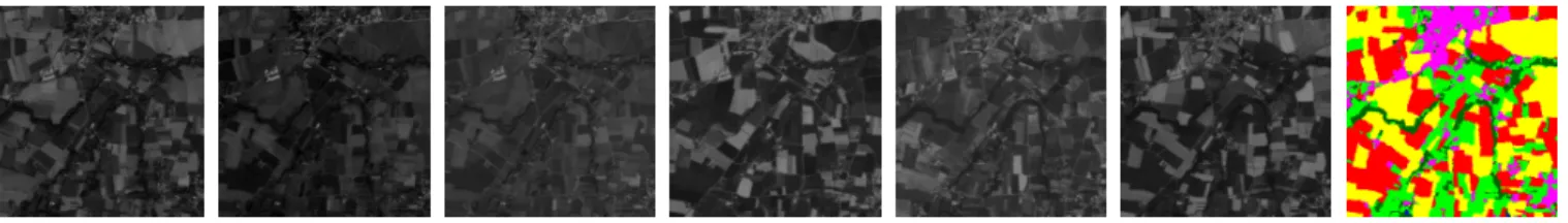
We illustrate the different strategies presented in Section 3 by some quantitative evaluation of land cover mapping. To do so, we consider the France Land Cover Map provided by [11] as a ground truth. More precisely, we give in Figure 2 (right color image) the cropped map that covers our sample SITS. The latter is made of 6 images acquired by Sentinel 2 over the west of France during 2017 within one month interval ap-proximately (shown chronologically on the left of Figure 2). The image size is 300 × 300 pixels and the spatial resolution is 10m. As already stated, we focus here on gray scale image so only one band was kept from the images. The region under study includes 5 land cover classes: summer crops (yellow), winter crops (red), urban area (pink), forest (dark green) and grasslands (light green). The min and max-trees are built us-ing iamxt [12], a Python open source toolbox.
For classification purpose, we randomly selected 100 pix-els from each class for training. The remaining pixpix-els were considered for testing. The thresholds related to the moment of inertia have been defined according to the literature as λ = (0.2, 0.3, 0.4). 3 area thresholds were randomly selected for every approach. As far as classification methods are con-cerned, we set the number of trees in RF to 100 and opt for the ’liner kernel’ in SVM. The 10-connectivity was used to build the spatial-temporal tree.
It is important to note that the length of the feature vec-tors depends on the size of the input data. While the two first strategies (tree for each date and spatial-temporal tree) led to 48 features per pixel, the third one (spatial extent tree) pro-vides only 13 features for each location.
We report in Table 1 the individual accuracies. The marginal approach (Section 3.1 and spatial-temporal model (Section 3.2 give better result, but at a higher cost in terms of feature length. Random Forest performs generally better than SVM. The preliminary results showed that AP increases the classification accuracy except when using the lexicographical
Fig. 2: From left to right: SITS frames and colored ground truth
ordering approach, illustrating the fact that the theoretical correctness does not always come with a practical usefulness.
Method RF-Area RF-Moment SVM-Area SVM-Moment
Without Tree 67 67 68 68 Marginal-AP 70 68 68 54 Spatial-Temporal AP 72 63 63 65 Lexicographic AP 59 63 54 59 DTW AP 68 68 59 61 Mean AP 67 68 62 61
Table 1: Comparison of overall classification accuracy
5. CONCLUSION
In this paper, we have proposed different approaches to adapt attribute profiles to satellite image time series. In order to deal with spatial information, we calculated area and moment of inertia attributes of the tree nodes. Experimental results show that proposed method give promising results for land cover mapping of SITS. Future work will deal with to take into account spectral information which increases the dimen-sion of information from three (2D spatial and temporal) to four. To produce feature profiles is another state-of-the-art strategy in MM. It could lead to better results for applications such as land cover classification. Besides, selection of opti-mal thresholds are needed for further works.
6. ACKNOWLEDGEMENT
The authors would like to thank Kalideos1 for providing the
Sentinel 2 dataset used in this study.
7. REFERENCES
[1] C. G´omez, J.C. White, and M.A. Wulder, “Optical re-motely sensed time series data for land cover classifica-tion: A review,” ISPRS J., vol. 116, pp. 55–72, 2016.
[2] P. Ghamisi, M. Dalla Mura, and J.A. Benediktsson, “A survey on spectral–spatial classification techniques based on attribute profiles,” IEEE TGRS, vol. 53, no. 5, pp. 2335–2353, 2015.
1https://bretagne.kalideos.fr
[3] M. Pesaresi and J.A. Benediktsson, “A new approach for the morphological segmentation of high-resolution satellite imagery,” IEEE TGRS, vol. 39, no. 2, pp. 309– 320, 2001.
[4] M. Dalla Mura, J.A. Benediktsson, B. Waske, and L. Bruzzone, “Morphological attribute profiles for the analysis of very high resolution images,” IEEE TGRS, vol. 48, no. 10, pp. 3747–3762, 2010.
[5] P. Bosilj, E. Kijak, and S. Lef`evre, “Partition and inclu-sion hierarchies of images: A comprehensive survey,” Journal of Imaging, vol. 4, no. 2, pp. 33, 2018.
[6] M.T. Pham, S. Lef`evre, E. Aptoula, and L. Bruzzone, “Recent developments from attribute profiles for remote sensing image classification,” in ICPRAI, 2018.
[7] G. Cavallaro, M. Dalla Mura, J.A. Benediktsson, and A. Plaza, “Remote sensing image classification using attribute filters defined over the tree of shapes,” IEEE TGRS, vol. 54, no. 7, pp. 3899–3911, 2016.
[8] M.A. Westenberg, J. Roerdink, and M.H.F. Wilkinson, “Volumetric attribute filtering and interactive visualiza-tion using the max-tree representavisualiza-tion,” IEEE TIP, vol. 16, no. 12, pp. 2943–2952, 2007.
[9] E. Aptoula and S. Lef`evre, “A comparative study on multivariate mathematical morphology,” Pattern Recog-nition, vol. 40, no. 11, pp. 2914–2929, 2007.
[10] M.T. Pham, E. Aptoula, and S. Lef`evre, “Feature pro-files from attribute filtering for classification of remote sensing images,” IEEE JSTARS, vol. 11, no. 1, pp. 249– 256, 2018.
[11] J. Inglada, A. Vincent, M. Arias, B. Tardy, D. Morin, and I. Rodes, “Operational high resolution land cover map production at the country scale using satellite image time series,” Remote Sensing, vol. 9, no. 1, pp. 95, 2017.
[12] R. Souza, L. Rittner, R. Machado, and R. Lotufo, “iamxt: Max-tree toolbox for image processing and analysis,” SoftwareX, vol. 6, pp. 81–84, 2017.