HAL Id: hal-00876194
https://hal.archives-ouvertes.fr/hal-00876194
Submitted on 24 Oct 2013
HAL is a multi-disciplinary open access
archive for the deposit and dissemination of
sci-entific research documents, whether they are
pub-lished or not. The documents may come from
teaching and research institutions in France or
abroad, or from public or private research centers.
L’archive ouverte pluridisciplinaire HAL, est
destinée au dépôt et à la diffusion de documents
scientifiques de niveau recherche, publiés ou non,
émanant des établissements d’enseignement et de
recherche français ou étrangers, des laboratoires
publics ou privés.
Fast Image Drift Compensation in Scanning Electron
Microscope using Image Registration.
Naresh Marturi, Sounkalo Dembélé, Nadine Piat
To cite this version:
Naresh Marturi, Sounkalo Dembélé, Nadine Piat. Fast Image Drift Compensation in Scanning
Elec-tron Microscope using Image Registration.. IEEE International Conference on Automation Science
and Engineering, CASE’13., Jan 2013, United States. pp.1-6. �hal-00876194�
Fast Image Drift Compensation in Scanning Electron Microscope Using
Image Registration
Naresh Marturi, Sounkalo Demb´el´e and Nadine Piat
Abstract— Scanning Electron Microscope (SEM) image ac-quisition is mostly affected by the time varying motion of pixel positions in the consecutive images, a phenomenon called drift. In order to perform accurate measurements using SEM, it is necessary to compensate this drift in advance. Most of the existing drift compensation methods were developed using the image correlation technique. In this paper, we present an image registration-based drift compensation method, where the correction on the distorted image is performed by computing the homography, using the keypoint correspondences between the images. Four keypoint detection algorithms have been used for this work. The obtained experimental results demonstrate the method’s performance and efficiency in comparison with the correlation technique.
I. INTRODUCTION
A SEM is a well-known tool for imaging the samples with submicrometer spatial dimensions. Apart from its nano-range imaging capabilities, a SEM can also be used in performing dynamic analysis and characterization of materials to recover their structural, mechanical, electrical and optical properties [1]. Besides material characterization, it is also used for sample preparation in desktop laboratories. Moreover, in vision-based autonomous micro-nanoassembling tasks, SEM images are used to provide dynamic visual feedback in assembling the microparts [2]. All these applications require long operational time and a varying magnification to fit the accuracy of measurements.
The SEM image acquisition process is heavily sensitive to time, especially at high magnifications. This is mainly due to the occurrence of drift in the images, that can be characterized as the evolution of pixel positions from time to time. Potential causes of this drift can be mechanical instability of the column or the sample support, thermal expansion and contraction of the microscope components, accumulation of the charges in the column, mechanical disturbances etc. However, in order to perform accurate measurements or manipulations using SEM, this drift has to be compensated beforehand.
In the literature, several methods have been proposed to es-timate and compensate the drift. A digital image correlation-based method for estimating the drift is used in [3], [4]. In This work is conducted with a financial support from the project NANOROBUST (ANR- 11-NANO-006) funded by the Agence Nationale de la Recherche (ANR), France. It is also performed in the framework of the Labex ACTION (ANR-11-LABX-01-01) and the Equipex ROBOTEX (contract ANR-10-EQPX-44-01) projects.
Naresh Marturi, Sounkalo Demb´el´e, and Nadine Piat are with Automatic control and Micro Mechatronic Systems (AS2M) depart-ment, Institute FEMTO-ST, Besanc¸on, France.naresh.marturi at femto-st.fr
[5], [6] and [7], a frequency domain phase correlation method is used. Cornille has proposed that the drift between pixels or between lines of an image is negligible; instead, the drift between the two images can be considered as a whole [3].
In general, two approaches are possible for drift com-pensation. The first one is based on estimating the drift directly from the current image by comparing it with a reference image and correcting the current image in real time [5], [7]. The second approach is based on develop-ing an empirical model of the drift that is then used to estimate and compensate the drift in real time [3], [4]. This approach is limited by its difficulty in computing a generic model. In this paper, using the first approach, the problem of drift compensation has been treated as an image registration problem between the images. It is performed using the keypoint detection methods and by computing the homography using the keypoint correspondences between the current and reference images.
The rest of the paper is organised as follows: Section II introduces to the problem of drift. Section III provides the details regarding the image registration using homography. The used methods to estimate the drift are presented in Sec-tion IV. Finally, the used experimental setup and the obtained results are presented in Sections V and VI respectively.
II. PROBLEM DESCRIPTION
In SEM, the images are formed by raster scanning the sample surface by means of a focused beam of electrons. When this beam interacts with the sample surface, the incident electrons are greatly scattered resulting in elastic and inelastic scattering [1]. Elastic scattering results in back scattered electrons (BSE) whereas inelastic scattering produces secondary electrons (SE), auger electrons and X-rays. The resulted electrons are recorded at their respective detectors and the gathered information is converted and saved as an image. The intensity value (I) of a pixel depends on the interaction position of the beam on the sample surface. For a scan length (N ) on the sample surface, the generation of one raster line (R) is given by (1).
Rn= N
X
i=1
I(xn, yi) (1)
where, n = [1 . . . M lines], x and y are the row and column indices of the interaction point. The total time taken (tn) to
produce one raster line is given by (2).
500 nm 500 nm
Fig. 1. Images of gold on carbon sample acquired at two different times. where, tp is the time to produce one pixel given by tD+ td,
tD is the dwell time i.e. the time taken by the beam to scan
one pixel, td is the time delay between the pixels and tld
is the line delay between two raster lines. At n = M , tn
becomes the time to produce one single scan image. The above equations hold well at ideal conditions.
However, in normal conditions, the instabilities present inside the SEM electron column add time-varying distortion (drift) and spatially-varying distortion to the images. The spa-tial distortion is constant in time and its calibration process is presented in [8]. On the other hand, drift occurs during the time of image acquisition and results in the pixel dis-placement. It is usually observed with consecutive scans even though there is no change in the device parameters. Most significantly, it affects the images at high magnifications. Fig. 1 shows two images of a gold on carbon sample acquired at different times at 18,000× magnifications, without changing any system parameters. By observing the two images, it is clear that the bright spot (inside the black rectangle) in the lower half of the first image is almost moved to the center position in the second image. This is the physical idea of the drift in x and y planes of the sample surface. Even though there exist the drift in z direction, it has a little impact on the image focus, so it is not considered in this paper.
III. IMAGE REGISTRATION
In image processing, image registration is the determi-nation of geometrical transformation to align two different images of a same view. Let I0and Itare two SE images of a
sample acquired at two different times t0and t1respectively.
Here, It has an unwanted motion (drift) with respect to
I0 and need to be compensated. Suppose, p0(x, y) ∈ I0
and p1(x0, y0) ∈ It are two pixels, one from each image,
the motion between them can be visually reflected by a homography (H) between both images and is given by (3). p0' Hp1 (3)
where, H is a 3×3 full rank matrix whose elements represent various degrees of freedom. By considering a non-zero value, ω, (3) is rewritten as in (4). ω x0 y0 1 = H11 H12 H13 H21 H22 H23 H31 H32 1 x y 1 (4)
Now, obtaining the corrected image ˆI, corresponds to the registration of Itwith respect to I0. This can be performed
in two ways: forward mapping and inverse mapping. Using forward mapping, for each pixel p1∈ It, the corrected pixel
Fig. 2. Experimental work flow diagram. ˆ
p ∈ ˆI is obtained directly by copying p1 using H as given
by (5).
ˆ
p = Hp1 (5)
In this case, some pixels in the corrected image might not get assigned, and would have to be interpolated. This problem could be solved using the second approach, inverse mapping given by (6).
p1= H−1ˆp (6)
Using this technique, the position of each corrected pixel ˆ
p is given and the mapping is performed by sampling the correct pixel p1 from the current image. In this work,
reverse mapping is used for the correction process. The block diagram depicting the overall process is shown in Fig. 2.
IV. DRIFT ESTIMATION A. Keypoints detection-based method
Keypoints detection and matching algorithms form the ba-sis for many computer vision problems like image stitching, data fusion, object recognition etc. The underlying idea with this technique is to extract distinctive features from each im-age, to match these features for global correspondence and to estimate the motion from the images. The overall task of drift compensation using this method is decomposed into four subtasks: keypoint detection, keypoint description, keypoint matching and homography estimation for correction.
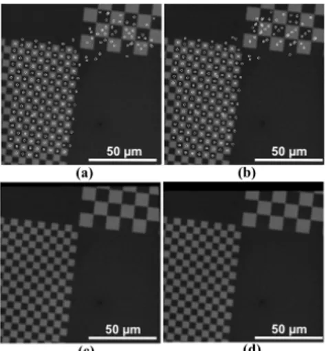
1) Keypoint detection: In this step, interest points are identified from both reference and current images such that the computed points should be same in both images. For this work, four keypoint detection algorithms (SURF, FAST, ORB and Dense) are used.
a) Speeded-up Robust Features (SURF) detector [9]: SURF detector is a Hessian-Laplacian-based detector. It detects the interest points by computing the Hessian matrix at various scales using box filters. This Hessian matrix corre-sponds to the Gaussian second order partial derivatives of the image. These points are then validated by the response of the determinant of Hessian matrix. Later, the scale and location of the points are refined using quadratic interpolation. Fig. 3(a) shows the keypoints detected using SURF detector.
b) FAST detector [10]: FAST is based on the corner points detection in the image. It computes keypoints directly on the image by searching for the pixels that are lying on the Bresenham circle with a selected radius. Then the absolute differences between these point intensities and the center pixel intensity of the circle are computed. The keypoints are the one having the difference greater than a selected threshold. Fig. 3(b) shows the detected keypoints. This method is known to be one of the fastest keypoint detection algorithms.
Fig. 3. Keypoints computed using (a) SURF (b) FAST (c) ORB and (d) Dense feature detectors applied on a microscale chessboard pattern.
c) Oriented FAST and Rotated BREIF (ORB) detector [11]: This detector is similar to FAST and a good alternative with an added orientation component. It uses a Harris corner measure to eliminate the edge response of the keypoints detected by FAST. Fig. 3(c) shows the detected keypoints.
d) Dense correspondence: Unlike the above keypoint detectors, this method uses dense sampling to produce a constant number of keypoints, covering the entire image (see Fig. 3(d)). An important disadvantage associated with this method is, it cannot achieve the level of repeatability in producing the same features as obtained by the other detectors.
2) Keypoint description: In this step, all the regions around the detected keypoints from the previous step are converted into compact and stable (invariant) descriptors, that can be matched against other descriptors. These descriptors contain information that can be used out of their respective regions. The output of this step is a feature vector s that will be used for matching. For this work, two keypoint descriptors, SURF and ORB are used.
a) SURF descriptor: This descriptor is used only with the keypoints identified using SURF detector. After identify-ing the keypoints, the detector assigns an orientation vector to each point. The descriptor is then constructed using this orientation vector and by dividing the region around each keypoint into subregions. For all these subregions, wavelet responses are computed and the sum of the horizontal and vertical responses produce the descriptor vector.
b) ORB descriptor: ORB descriptor is an extension technique of BRIEF descriptor. For the detected keypoints, assuming that the corner’s intensity has an offset from its center location, an orientation vector is computed from the corner’s center to the centroid. This vector is then assigned to the keypoint and used in producing the descriptor.
3) Keypoint matching: The next step is to match the corresponding features at different locations obtained from the above steps. One way is by computing the Euclidean distance d between the feature vectors s1and s2in the feature
space given by (7). d(s1, s2) = X i (s1i− s2i)2 !12 (7)
Having the Euclidean distance, matching is accomplished by setting a threshold and by returning all the matches less than this value in the images. However, using a large value for the threshold may result in false matches. The other way is to simply match the nearest neighbours (smallest d) in the images. This eliminates the problem associated with the previous method. In this work, nearest neighbour-based matching has been used.
4) Homography estimation: The final step is to estimate the drift using the information obtained from above step. After performing the matching, we get K keypoint corre-spondences in both images. In this situation, homography is estimated using an iterative method, random sample con-sensus (RANSAC) [12]. This method is summarized in the below steps.
1) Choose four random keypoint correspondences from the available ones.
2) Compute homography that maps the four points ex-actly to their corresponding points.
3) Find a consensus set for the computed homography by calculating the inliers i.e. find other keypoint corre-spondences such that their distances from the current model are small.
4) Repeat the step 3 for certain iterations fixed by a threshold and choose the homography (H) with largest consensus set (set of inliers).
5) Finally, recompute H using all the points in the con-sensus set.
Once H is computed, the correction is performed on the current image as mentioned earlier in Section III.
B. Phase correlation method
This is the most common approach for estimating the drift in SEM images. In this paper, we use this method for comparing the results obtained from the feature-based methods. The underlying idea behind this method is quite simple and is based on the Fourier shift property. It states that the shift in the coordinate frames of two images in the spatial domain can be realized as the linear phase differences in the Fourier domain. Assuming that I0(x, y) and It(x0, y0)
are two different SE images acquired at times t0 and t1
respectively and are shifted by (δx, δy).
It(x0, y0) = I0(x + δx, y + δy) (8)
The Fourier transforms for both images are given by F0(u, v)
and Ft(u0, v0) computed as shown in (9).
F0(u, v) = M −1 X x=0 N −1 X y=0 I0(x, y)e−j2π{ ux M+ vy N} (9)
where, M and N correspond to image dimensions, x and y are the pixel coordinates. Now, according to the Fourier shift property
Ft(u0, v0) = F0(u, v)e−j2π{
u
Mδx+Nvδy} (10)
The normalized cross power spectrum, R(u, v) can be com-puted using F0(u, v) and the complex conjugate Ft(u0, v0)
as given by (11).
R(u, v) = F0(u, v)Ft(u
0, v0)
| F0(u, v)Ft(u0, v0) |
= ej2π{Muδx+Nvδy} (11)
There are two ways to solve (11) for computing the drift (δx, δy). The first one is to directly work in the Fourier
domain by defining three axes (two frequency and one image phase difference) and solving for the slopes given by Muδx+
v
Nδy= 0 along the frequency axes. These slopes provide the
drift in the images. But this way is computationally complex. The second and more practical method that is used in this work is to find the inverse Fourier transform of (11), that results in a Dirac delta function G(δx, δy) given by (12).
G(δx, δy) = F−1{R(u, v)} (12)
Finally, the global drift (∆x, ∆y) is the maximum value of
(12). Again, the correction is performed using homography. In this case, the matrix H contains only the translation information and is given by (13).
H = 1 0 ∆x 0 1 ∆y 0 0 1 (13) This method of computing the drift has a remarkable advantage over the traditional cross-correlation techniques; that is its accuracy in finding the peak of correlation at the point of registration. However, this technique can be used only if the motion between two images is a pure translation. In case of rotation, phase correlation produces multiple peaks. Fig. 4 shows the phase correlation peak of the two images shown in Fig. 1.
V. EXPERIMENTAL SETUP
The experimental setup architecture used for this work is shown in Fig. 5. It consists of a JEOL JSM 820 SEM along with two computers. The SEM electron column consists of an electron gun with tungsten (W) filament, an anode, an objective aperture, a secondary electron (SE) detector, two scan coils, an objective lens and a vacuum chamber equipped with a movable platform to place the sample. The possible magnification with the SEM ranges from 10× to 100, 000×. The primary computer (Intel Pentium 4, CPU 2.24 GHz and 512 MB of RAM) is solely responsible for
Fig. 4. Phase correlation of the images shown in Fig. 1.
SEM control and it is connected to the SEM electronics and an image acquisition system (DISS5 from Point Electronic). The second PC (Intel Core 2 Duo, CPU 3.16 GHz, and 3.25 GB of RAM) is connected to the primary one using an Ethernet crossover cable. The communication between the two PCs is accomplished using a client - server model, where the server program runs on the primary computer. The server is mainly responsible for acquiring the images and transfer them to the client. On the other side, image client receives these images and performs the drift compensation.
VI. EXPERIMENTAL RESULTS
The experiments with the system are carried out using a standard gold on carbon sample with the particle size up to 500 nm (see Fig. 6(a)) and a microscale calibration rig (silicon) containing chessboard patterns (see Fig. 6(b)) designed at FEMTO-ST. The acceleration voltage used to produce the beam is 15 kV for gold on carbon sample and 10 kV for the calibration rig. The electronic working distance is set to 6.2 mm and 4.7 mm for both the samples respectively in order to keep the sample surface in focus. All tests are performed using SE images with a size of 512 × 512 pixels. The tD is set to 360 ns to get an image
acquisition speed of 2.1 frames per second. This speed could be increased, but at high scan speeds the image noise is more.
A. Methods evaluation
Initial experiments have been performed to evaluate the two different methods of drift compensation explained in section IV. The final goal of this test is to find a method that provides good accuracy and speed in compensating the drift. Gold on carbon sample images acquired after
900-Fig. 5. Experimental setup architecture.
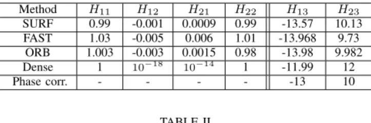
TABLE I
HOMOGRAPHY PARAMETERS COMPUTED AT10,000×MAGNIFICATIONS. Method H11 H12 H21 H22 H13 H23 SURF 0.99 -0.001 0.0009 0.99 -13.57 10.13 FAST 1.03 -0.005 0.006 1.01 -13.968 9.73 ORB 1.003 -0.003 0.0015 0.98 -13.98 9.982 Dense 1 10−18 10−14 1 -11.99 12 Phase corr. - - - - -13 10 TABLE II
HOMOGRAPHY PARAMETERS COMPUTED AT20,000×MAGNIFICATIONS. Method H11 H12 H21 H22 H13 H23 SURF 1.004 0.0009 0.001 0.99 1.003 10.54 FAST 0.99 0.004 0.002 0.99 0.73 10.66 ORB 0.97 0.001 0.002 0.94 0.98 10.49 Dense 1 10−16 10−12 1 2.0 11.51 Phase corr. - - - - 1 10
seconds from the reference image at 10, 000× and 20, 000× magnifications are used for the evaluation process.
Fig. 7(a) and Fig. 7(c) show the reference images acquired at 10, 000× and 20, 000× magnifications respectively. The drift compensation has been carried out using all the ex-plained methods. Fig. 7(b) and Fig. 7(d) show the corrected images at 10, 000× and 20, 000× magnifications respectively using ORB detector. The black region observed in the borders of the corrected images is due to the compensated drift. Table I and Table II shows the computed homography using all methods at 10, 000× and 20, 000× magnifications respec-tively. The first four columns (H11, H12, H21, H22) provide
the rotation information and the last two columns (H13, H23)
provide translation. The region of interest (ROI) within the black square shown in every image is used for computing the accuracy of drift correction i.e. to measure how close the corrected image is with the reference image. This is performed by calculating the mean square error (MSE) given by (14) between the reference and corrected ROIs.
EM SE = 1 M N X M X N (IROI− ˆIROI)2 (14)
where, IROI and ˆIROI are the regions of interest from
reference and current images respectively. The results are summarized in Table III. Fig. 8(a) and 8(b) show the disparity maps computed using the reference and corrected images ROI at 10,000× and 20,000× magnifications respectively. These maps provide the relative displacement between the pixels in two images after correction. The total time taken to estimate and correct the drift for one image is shown in Table. IV (implemented in c++).
Tests are also performed to compensate the drift in real time experiments using the calibration rig at 2000× magnifi-cations. Fig. 9(a) and Fig. 9(b) show the keypoints obtained from reference image and current image and Fig. 9(c) and Fig. 9(d) show corrected images at different times.
From the obtained results, ORB keypoint detector-based method shows good speed and accuracy over the other meth-ods in compensating the drift. Even though, SURF-based method also shows good accuracy in correcting the drift; it
TABLE III
MSEAT10,000×AND20,000×MAGNIFICATIONS. Method MSE 10,000× 20,000× SURF 7.1441 8.2584 FAST 7.7011 8.9798 ORB 7.1978 8.4198 Dense 34.9347 25.5286 Phase correlation 11.0914 17.3596 TABLE IV
TOTAL TIME TAKEN FOR DRIFT COMPENSATION. Method Time (ms) SURF 871 FAST 92 ORB 31 Dense 1469 Phase correlation 78
takes more time for computation. Thus, making it difficult to use with real-time applications. Moreover, all keypoint-based methods (except dense) show better performance than the phase correlation method. The major advantage associated with these methods is that the correction can be performed with subpixel accuracy in both rotation and translation. However, these methods are sensitive to the image noise. So the image quality is monitored continuously during the overall process using the method proposed in [13].
B. Computing the evolution of drift
Different tests have been performed to evaluate the path followed by the drift at various magnifications. For this test, a series of gold on carbon sample images are acquired for different magnifications ranging from 10,000× to 20,000× with a step change of 1000×. For each magnification, 30 images are acquired at a rate of one image for every 30-seconds. ORB detector-based method is used for this test. Fig. 10 and Fig. 11 show the evolution of drift (in pixels) with respect to x and y axes respectively at various magnifications. From the obtained results, it is observed that the drift
Fig. 7. (a) and (b) Reference and corrected images at 10K× magnification. (c) and (d) Reference and corrected images at 20K× magnification. Cor-rected using ORB detector method. The black square is the selected ROI. Black region on the borders is the drift displacement after 900s.
Fig. 8. Disparity maps computed using the reference and corrected image ROIs at (a)10,000× and (b)20,000× magnifications.
Fig. 9. (a) and (b) Keypoints computed from reference and current images (c) and (d) corrected images at different times using ORB method. produced in the images is only a translation in x and y axes and no rotation is involved (from Tables I and II). The path followed by the drift in x and y axes can be approximated with a linear motion. It is also observed that the velocity of drift increases with time as the number of pixels evolving is more at higher times. It is assumed that this drift is a result of the motion produced by the sample stage motors because of the thermal variations inside the chamber over time. However, rotation in the drift can be observed only when there is a change in the focus which is a result of the variations in electromagnetic field produced by the lens. This type of drift can be characterized as the motion in z axis, because the focus can be varied by displacing the sample stage in z direction.
VII. CONCLUSIONS
In this paper, a new image registration-based drift compen-sation method has been implemented utilizing the keypoints detection and matching technique. Four keypoint detection algorithms have been tried in this work and out of all, ORB detector showed the better speed and accuracy in computing the drift. Later, the drift correction has been performed on the distorted image using the homography computed from the keypoint correspondences. Unlike the classical correlation based methods, the implemented method has an ability to correct the rotation, shear and scaling. Besides, from the obtained results, we conclude that the drift corresponds to an inter-frame translation and no rotation is involved.
As part of future work, this study will be continued by analyzing the impact of change in SEM parameters like beam tilt, spot size etc. towards drift.
Fig. 10. Motion of the drift in x-axis at different magnifications.
Fig. 11. Motion of the drift in y-axis at different magnifications. REFERENCES
[1] J. Goldstein, D. E. Newbury, D. C. Joy, C. E. Lyman, P. Echlin, E. Lifshin, L. Sawyer, and J. R. Michael, Scanning electron microscopy and X-ray microanalysis. Springer, 2003.
[2] S. Fatikow, C. Dahmen, T. Wortmann, and R. Tunnell, “Visual feed-back methods for nanohandling automation,” International Journal of Information Acquisition, vol. 6, no. 03, pp. 159–169, 2009. [3] N. Cornille, “Accurate 3d shape and displacement measurement using
a scanning electron microscope,” Ph.D. dissertation, University of South Carolina, 2006.
[4] M. Sutton, N. Li, D. Joy, A. Reynolds, and X. Li, “Scanning electron microscopy for quantitative small and large deformation measurements part i: Sem imaging at magnifications from 200 to 10,000,” Experi-mental Mechanics, vol. 47, no. 6, pp. 775–787, 2007.
[5] A. C. Malti, S. Demb´el´e, N. Piat, C. Arnoult, and N. Marturi, “Toward fast calibration of global drift in scanning electron microscopes with respect to time and magnification,” International Journal of Optomechatronics, vol. 6, no. 1, pp. 1–16, 2012.
[6] Q. Yang, S. Jagannathan, and E. Bohannan, “Automatic drift compen-sation using phase correlation method for nanomanipulation,” IEEE Transactions on Nanotechnology, vol. 7, no. 2, pp. 209–216, 2008. [7] P. Cizmar, A. E. Vlad´ar, and M. T. Postek, “Real-time scanning
charged-particle microscope image composition with correction of drift,” Microscopy and Microanalysis, vol. 17, no. 2, p. 302, 2010. [8] A. C. Malti, S. Demb´el´e, N. Le Fort-Piat, P. Rougeot, and R. Salut,
“Magnification-continuous static calibration model of a scanning-electron microscope,” Journal of Electronic Imaging, vol. 21, no. 3, pp. 033 020–1, 2012.
[9] H. Bay, A. Ess, T. Tuytelaars, and L. Van Gool, “Speeded-up robust features (surf),” Computer vision and image understanding, vol. 110, no. 3, pp. 346–359, 2008.
[10] E. Rosten and T. Drummond, “Fusing points and lines for high performance tracking,” in Tenth IEEE International Conference on Computer Vision, vol. 2. IEEE, 2005, pp. 1508–1515.
[11] E. Rublee, V. Rabaud, K. Konolige, and G. Bradski, “Orb: an efficient alternative to sift or surf,” in IEEE International Conference on Computer Vision. IEEE, 2011, pp. 2564–2571.
[12] R. Hartley and A. Zisserman, Multiple view geometry in computer vision. Cambridge Univ Press, 2000, vol. 2.
[13] N. Marturi, S. Demb´el´e, and N. Piat, “Performance evaluation of scan-ning electron microscopes using signal-to-noise ratio.” International Workshop on MicroFactories, pp. 1–6, 2012.