A pattern reordering approach based on ambiguity detection for on-line category learning

Titre:

Title: A Pattern Reordering Approach Based on Ambiguity Detection for On-Line Category Learning Auteurs:

Authors: Éric Granger, Yvon Savaria et Pierre Lavoie Date: 2002

Type: Rapport / Report Référence:

Citation:

Granger, Éric, Savaria, Yvon et Lavoie, Pierre (2002). A pattern reordering approach based on ambiguity detection for on-line category learning. Rapport technique. EPM-RT-2001-02.

Document en libre accès dans PolyPublie Open Access document in PolyPublie

URL de PolyPublie:

PolyPublie URL: http://publications.polymtl.ca/2593/

Version: Version officielle de l'éditeur / Published version_{Non révisé par les pairs / Unrefereed} Conditions d’utilisation:

Terms of Use: Autre / Other

Document publié chez l’éditeur officiel Document issued by the official publisher

Maison d’édition:

Publisher: École Polytechnique de Montréal

URL officiel:

Official URL: http://publications.polymtl.ca/2593/

Mention légale:

Legal notice: Tous droits réservés / All rights reserved

Ce fichier a été téléchargé à partir de PolyPublie, le dépôt institutionnel de Polytechnique Montréal

This file has been downloaded from PolyPublie, the institutional repository of Polytechnique Montréal

EPIWRT-0 1/02

A Pattem Reordering Approach Based on Ambiguity Detection for On-Line Category Learning

Éric Granger Yvon Savaria Pierre Lavoie

Département de génie électrique

02001-09

Éric Granger, Yvon Savaria, Pierre Lavoie Tous droits réservés

Dépôt légal :

Bibliothèque nationale du Québec, 2001 Bibliothèque nationale du Canada, 200 1 EPM-RT-O 1/02

A Pattern Reordering Approach Based on Ambigu@ Detection for On-Line Category Learning

par : Éric Granger, Yvon Savaria et Pierre Lavoie Département de génie électrique

Ecole Polytechnique de Montréal

Toute reproduction de ce document à des fins d’étude personnelle ou de recherche est autorisée à la condition que la citation ci-dessus y soit mentionnée.

Tout autre usage doit faire l’objet d’une autorisation écrite des auteurs. Les demandes peuvent être adressées directement aux auteurs (consulter le bottin sur le site http://www.polymtl.ca) ou par l’entremise de la Bibliothèque :

École Polytechnique de Montréal

Bibliothèque - Service de fourniture de documents Case postale 6079, Succursale « Centre-ville » Montréal (Québec)

Canada H3C 3A7

Téléphone : (5 14) 340-4846

Télécopie : (5 14) 340-4026

Courrier électronique : biblio.peb@,courriel.polvmtl.ca

Pour se procurer une copie de ce rapport, s’adresser à la Bibliothèque de l’École Polytechnique. Prix : 25.00$ (sujet à changement sans préavis)

Régler par chèque ou mandat poste au nom de l’École Polytechnique de Montréal.

Toute commande doit être accompagnée d’un paiement sauf en cas d’entente préalable avec des établissements d’enseignement, des sociétés et des organismes canadiens.

A Pattern Reordering Approach Based on Ambiguity

Detection for On-Line Category Learning

Eric Granger

, Yvon Savaria

and Pierre Lavoie

1

_{Defence Research Establishment Ottawa}

Dept. of National Defence

Ottawa, Ontario, Canada

2

_{Dept. of Electrical and Computer Eng.}

´Ecole Polytechnique de Montr´eal

Montreal, Quebec, Canada

reject option.

Abstract

Pattern reordering is proposed as an alternative to sequential and batch processing for on-line category learning. Upon detecting that the categorization of a new input is ambiguous, the input is postponed for a predefine time, after which it is reexamined and categorized for good. This approach is shown to improve the categorization performance over purely sequen-tial processing, while yielding a shorter response time, or latency than batch processing. The latency of a typical implementation is derived and compared to lower bounds. Gaussian and softmax models are derived from reject option theory, and are considered for detecting ambi-guity and triggering pattern postponement. The latency and Rand Adjusted score of reordered, sequential and batch processing are compared through computer simulation with Gaussian and Iris data sets.

3_{Corresponding author: Defence Research Establishment Ottawa, 3701 Carling Ave., Ottawa, Ontario, K1A 0Z4,}

1 Introduction

A number of pattern recognition applications involve high throughput category learning from con-tinuous streams of input patterns. In pattern recognition literature, partitional clustering tech-niques [2] [11], such as on-line versions of the k-means [34] and leader [25] algorithms, are pro-posed for on-line category learning. Other algorithms include on-line versions of adaptive vector quantization (AVQ) [18] [20] (e.g., generalized Lloyd [33] and Linde-Buzo-Gray (LBG) [31] algo-rithms) in communication theory, and unsupervised competitive learning (UCL) [21] [22] [23] [30] (e.g., standard UCL networks [1] [10] [35] and Adaptive Resonance Theory (ART) networks [5]) in neural network theory. These algorithms learn input patterns autonomously on the fl , some without prior knowledge of the number and characteristics of categories. The above algorithms do not require long-term storage of input patterns, and lend themselves well to high throughput, parallel implementation.

A common trait of these algorithms is their sequential processing of input patterns. When an input pattern is presented, it is compared to the prototype of every category. The category with the best matching prototype (according to some similarity measure) is assigned to the input, and the prototype of this category adapts to novel characteristics of the input. Over a succession of inputs, category prototypes become tuned to different parts of the input space, and implicitly defin inter-category decision boundaries. Therefore, the unknown probability density function of the data source is progressively estimated using a finit number of prototypes.

With sequential processing, a fina decision is taken upon presentation of every input. This implies that, for each decision, only information from prior input patterns is available. In addition, the fact that prototypes are stored rather than prior input patterns implies that learning — the

consequence of each decision — is irreversible. Information is therefore lost in the process. Limitations of sequential processing are obvious, particularly if the structure of input data clusters tends to be scattered and/or overlapping. For instance, if upon its presentation, an input pattern lies in proximity to a decision boundary separating two or more categories, the clusterer is forced to make a fina decision, despite the ambiguity. Irreversible learning for such decisions gives rise to different category structures, and diverging decision boundaries that vary significantl according to the pattern presentation order. Thus, clustering quality depends largely on the context.

The quality of results is generally improved with batch processing. It consists of collecting and storing one batch of patterns from the input stream, while the clusterer converges iteratively, over several epochs, on a previously-accumulated batch of patterns. An epoch is one complete presentation of the fi ed-size batch of data, one pattern at a time, to the clusterer. Convergence is attained when the prototypes remain constant for two successive epochs. Batch processing can diminish or eliminate sensitivity to the input presentation order by allowing the clusterer, for example, to recover from some early miss-assignments caused by exposure to ambiguity. Although this approach can yield better results, it entails delays caused by the accumulation of patterns to form batches, and requires data buffering to account for the variability of the computational effort. In this paper, an alternative called reordered processing is proposed for on-line category learn-ing. As a clusterer assigns categories to input patterns, it is granted the ability to postpone, or delay, the categorization (category assignment and learning) when it detects an ambiguity. Delayed pat-terns are queued, and their categorization is deferred for some fi ed time. The overall effect is a modificatio to the order in which inputs are categorized. Aside from allowing to control the maximum response time, pattern postponement offers the opportunity to circumvent learning for

ambiguous decisions.

The rest of this paper is organized as follows. In Section 2, lower bounds on the latency re-quired for on-line category learning are developed for sequential, batch and reordered processing. Then, practical issues are discussed, and high-level architectures are proposed to implement batch and reordered processing. Elements of reject option theory are developed for the detection of am-biguous category assignment in Section 4. The experimental methodology, and proof-of-concept computer simulations using three neural networks are presented and discussed in Section 5. It is shown that the proportion of patterns that are declared ambiguous is a good indicator of poor clustering quality; and that modifying the order in which input patterns are processed, based on ambiguity detection, can enhance clustering quality for a moderate increase in latency. Finally, reordered processing offers an interesting alternative to batch processing in terms of trading off clustering quality versus response time.

2 Latency in on-line category learning

On-line category learning of a continuous stream of input patterns is performed by a clusterer (e.g., an on-line k-means algorithm) which is exploited through one of several data processing schemes. Given our focus on high throughput applications, the input response time incurred by adopting a data processing scheme is a critical consideration. Let input patterns to be categorized arrive one at a time from some source that provides them at a rate that need not be constant. The latency L of

the category learning is define as the number of input patterns subsequent to an input a that are

necessary before a fina decision (category)y a can be assigned to a. By neglecting the response

characterized. Lower bounds on the minimum, maximum and average latency required for three data processing schemes — sequential, batch and reordered — are now examined.

A basic approach to learning a continuous data stream is through sequential processing. Upon

observation of each input patterna, a category can be assigned to a without waiting for subsequent

patterns.

Batch processing consists in categorizing the input patterns a in fi ed-size batches of k

pat-terns. Incoming patterns are accumulated until a group of k successive patterns has been formed. The following patterns are buffered while the previous k patterns are being learned. Batches of incoming data are learned iteratively, over several epochs, until convergence is attained. The

cat-egory assigned to each patterna in a batch is produced once convergence has been detected, i.e.,

upon the last one of these epochs.

Reordered processing consists in postponing the learning of input patternsa for which category

assignment is deemed ambiguous. Each postponed pattern is queued, and categorized following a fi ed latency of d patterns. To bound the latency of reordered patterns, a given pattern can only be postponed once.

The minimum latency Lmin for all three data processing schemes must satisfy:

Lmin 0 (1)

being postponed with reordered processing. The maximum latency Lmax must satisfy: Lmax 0 ; sequential processing, k 1 ; batch processing, d ; reordered processing, (2)

where k is the number of patterns per batch, and d is the user-define queue size. This lower bound

corresponds toa being the firs pattern in a batch with batch processing, or a being postponed with

reordered processing. Lastly, it is straightforward to show that the average latency L is:

L 0 ; sequential processing, 1 k k i 1 k i ; batch processing, pr a d ; reordered processing, (3)

where pr a is the pattern rejection, or postponement rate. This rate depends on the data structure

and the rejection criterion.

Reordered processing constitutes a compromise between sequential processing and batch

pro-cessing. Notice that if d k 1 and pr a 50%, then the lower bounds on Lmax and L are

equal for batch and reordered processing. If, on the other hand, d 0, then reordered processing reduces to sequential processing.

3 Practical clustering systems

In order to characterize the latency of clustering systems for on-line category learning, assume from

clusterer embedded within this system, the reported latency characterizes the overhead required with a data processing scheme. The rest of this section raises practical issues involved with the implementation of clustering systems, and describes high level architectures that can accommodate batch and reordered processing.

(a) batch processing architecture. (b) reordered processing architecture.

Figure 1: High level architectures of clustering systems for on-line clustering.

3.1 An architecture for batch processing

Batch processing involves incremental convergence over several batch epochs — the number of successive presentations of a batch of k patterns to the clusterer for convergence. The number of batch epochs required to attain the state of convergence varies from one batch to the next, according to the queue length k, as well as the structure of the specifi data patterns in the batch. The computational effort is therefore variable and somewhat unpredictable. The requirement for convergence is also costly, because at least one whole batch epoch of overhead is required to

detect the state of convergence, thus 2. Finally, accumulation of incoming data occurs until

the clusterer has converged for the current batch of patterns.

two identical fi ed-length queues of k registers that operate concurrently, and a clusterer that can

process each pattern within a fi ed time c. Using two parallel queues eliminates the clusterer’s

delay for accessing a new batch of data. Each queue alternates between a collection (A) and a processing (B) mode. While one of the queues temporarily buffers k incoming patterns from the input stream (A), the other queue stores a batch of k patterns being learned by the clusterer (B).

To circumvent the delay required for detection of convergence, the number of batch epochs,

, can be bound to a constant value across batches, 2. A fina decisiony a can be produced

immediately after processing ofa, as part of the last epoch. The processing rate must satisfy:

c a (4)

which imposes a processing rate constraint on the clusterer that is proportional to the number of batch epochs , and prevents overfl ws of the queue operating in collection mode.

Immediately after a queue is switched to the collection mode (A), a pattern a from the input

stream is stored every aseconds inside its registers. After k aseconds, the registers are full, and

the queue is switched into processing mode (B). In this mode, patterns are shifted right through

the clusterer every cseconds. A feedback loop allows repeated presentations. After epochs, the

registers are reset prior to switching back to collection mode. The latency of the batch processing architecture of Figure 1(a) is the sum of the delays incurred in both modes. In the best case, when

a is the last of a batch,

Lmin k (5)

and in the worst case, whena is the firs of a batch,

The average latency of this architecture is: L 1 k k i 1 k i 1 k i ₍₇₎

It is easily verifie that (5), (6) and (7) satisfy but do not meet the lower bounds (1), (2) and (3).

3.2 An architecture for reordered processing

With a clustering system that uses reordered processing, a pattern having been postponed by d patterns has priority over a pattern from the input stream. This ensures a fi ed worst-case response time of d patterns, but leads to the accumulation of up to d incoming patterns at the clustering system’s input. Also, a clusterer embedded within this system requires additional circuitry to detect ambiguity.

One possible architecture to implement reordered processing is shown in Figure 1(b). It con-sists of a fi ed-length queue composed of d registers, and a clusterer capable of detecting

ambigu-ous category assignments. If an input pattern a is deemed ambiguous, it is diverted towards the

queue and labeled a . Shifting this pattern through the queue is equivalent to a fi ed delay that

changes the presentation order.

Each pattern b that is processed by the clusterer is either a new input pattern, b a, or a

previously-rejected and therefore delayed pattern,b a . A simple way to schedule processing is

to assume that the clusterer’s processing time is partitioned into two equal time slices: one slice

reserved to process input patterns a, and the other slice reserved to process previously-rejected

patternsa . To allow alternating between the two sources, the augmented clusterer must be able to

process a patternb within a fi ed time of cthat satisfies

This speed constraint is similar to that of batch processing with 2. With proper synchronization, the need for an input buffer is avoided. With this architecture, the lower bounds (1), (2) and (3) are met.

4 Ambiguity in competitive learning assignments

With sequential processing, each input patterna that is presented to the clusterer is compared to the

prototypewjrepresenting category j, for j 1 2 N. The category j J with the best matching

prototype is assigned to inputa. Two forms of uncertainty can influenc this assignment.

Intra-category uncertainty accounts for the degree of mismatch between a and prototype wJ

of category J. For clusterers in which the number of categories N is fi ed (e.g., on-line k-means algorithm), this uncertainty can be reduced at the outset by using greater N values. By contrast, other clusterers (e.g., leader algorithm) regulate the maximum tolerable amount of intra-category uncertainty by imposing a minimum degree of match per assignment. If assignment of category J toa does not satisfy the matching threshold, then a new category is initialized to represent a.

Inter-category uncertainty or ambiguity accounts for the degree of match between a and the

prototypes of all N categories. Ambiguity grows asa lies closer to a decision boundary between

category J and any other category j 1 2 N, j J. The symptom of this is multiple prototypes

wjhaving an almost equal degree of match witha.

With reordered processing, ambiguity is employed as a criterion for postponing pattern catego-rization. The clusterer is equipped with the ability to detect ambiguity during category assignment (i.e., before prototype adjustment). The rest of this section concerns the measurement, from a statistical standpoint, of ambiguity. Given the focus on high throughput clustering, particular

em-phasis is placed on measures with low computational complexity.

4.1 Bayes decision theory and the reject option

In statistical pattern recognition, the reject option [7] [8] [16] provides a framework for detecting the ambiguous assignment of a class to an input pattern. By exercising an option to reject, a recognition system can abstain from making a meaningless classification and submit the rejected input pattern for exceptional handling such as manual inspection.

If the underlying statistics of the pattern recognition problem are fully known, the Bayes

deci-sion procedure assigns 1-out-of-N possible classes to input patterna using the maximum a

poste-riori probability decision rule:

J argmax p j a : j 1 2 N (9)

where 0 p j a 1 and N

j 1p j a 1. The a posteriori probability p j a that class j

generated inputa is computed according to the Bayes theorem:

p j a Pj p_p a j_{a N}Pj p a j

k 1Pk p a k ; j 1 2 N (10)

where Pjis the a priori probability of class j, with 0 Pj 1 and N_{j 1}Pj 1, p a j is the

condi-tional probability density function (p.d.f.) of the inputa given class j, and p a N

j 1Pj p a j

is the unconditional p.d.f. of inputa (mixture density function). Eq. (9) define decision boundaries

that yield the minimum probability of miss-classificatio [3] [13] [17].

The degree of ambiguity regarding the decision rule of Eq. (9) can be measured in terms of the

conditional error given inputa [7] [8] [12] [16]:

1 p J a N

j 1 j J p j a (11)

Assignment of class J to inputa is define to be ambiguous if rJ a is greater than or equal to a

rejection threshold 0 1 : rJ a (12) From Eq. (10): N j 1 j J Pj p a j N j 1 Pj p a j 1 PJ p a J N j 1 j J Pj p a j (13)

Since the conditional error givena ranges from rJ a 0 (the assignment is completely

unambigu-ous, with p J a 1) to rJ a N 1_N (the assignment is completely ambiguous or random, with

p J a 1

N), the rejection threshold must satisfy 0 N 1N to be consistent with Eq. (13).

Eq. (13) define a region of ambiguity, Lr a : rJ a , of the input space, that is, where

class assignments are considered to be ambiguous. The size of this region grows as is decreased.

For a given , the size of the region also depends on the shape of rJ a at the decision boundary of

class J, and hence on the class distribution in the input space. The rate of rejection is:

pr a

Lr p a da (14)

The option to reject patterns that fall in Lr provides a means of reducing the number of

classificatio errors. Patterns that would have been correctly classifie may also be rejected. The performance level of a pattern recognition system with reject option is therefore characterized by the trade-off between error and rejection rates [8] [16] [24].

4.2 Extensions for on-line category learning

In practical applications, the probabilities required to implement the reject option are usually un-known. They must be estimated based on a clusterer’s response to input patterns. A clusterer may be subjected to different environments, with more or less prior information on the underlying data structure. Two environments are now considered. In the first clusters of data are obtained from sources having identically distributed Gaussian distributions, where all variables are independent

and have equal variance 2_{. In the second, no prior assumption is made about the underlying input}

data structure, and data clusters are modeled implicitly. Eq. (13) is now developed for each one of these environments.

4.2.1 Gaussian rejection model

The result of on-line category learning can be interpreted as a model of the statistical distribution

of the input data. Assume that the probability distribution of the data p a can be modeled as a

mixture of conditional density functions p a j for j 1 2 N: p a N

j 1Pj p a j [3] [13].

Each component p a j corresponds to the probability of input a, given category j, whereas

mixing parameter Pj corresponds to the a priori probability of category j.

Assuming that the noise is Gaussian, the conditional density functions p a j are define by

independent normal distribution functions. In an M-dimensional space, the multivariate normal probability distribution is:

p a j 1

2 M2 _j 12 exp

1

2 a j T j1 a j (15)

where jand jare the mean vector and covariance matrix for category j. Therefore each category

If the data clusters are generated by sources with the same Gaussian noise, and all categories

have equal covariance matrices ( j for j 1 2 N), then the decision boundaries are

hy-perplanar. If all variables are statistically independent and have equal variance 2_{, then is a}

diagonal matrix ( 2_{I, where I is the identity matrix, and} M

i 1 2i 2M), and

distribu-tions are hyperspherical. Lastly, if all categories have equal a priori probabilities (Pj 1 N for

j 1 2 N), then the maximum a posteriori probability decision rule given in Eq. (9) reduces

to template matching: J argmax 1 N 2 2 M2 exp 1 2 a j T j1 a j : j 1 2 N argmax 1₂ M i 1 ai ji ji 2 : j 1 2 N argmin a j 2: j 1 2 N (16)

where a j is the Euclidean distance. Data clusters are therefore modeled explicitly as

hyper-spherical normal distributions, which constitute estimates of the conditional probabilities p a

j : j 1 2 N .

In light of the previous assumptions, the reject option of Eq. (13) is reduced to:

1 N 2 12 M2 exp 1 2 a J T J1 a J N j 1 j J_{N 2}1_{2 M2} exp 12 a j T j1 a j exp 1₂ M i 1 ai JiJi 2 N j 1 j Jexp 12 Mi 1 ai _jiji 2 exp a J 2 2 2 N j 1 j Jexp a2 2j 2 (17) Eq. (17) is define as the Gaussian rejection model for detecting ambiguous category assignments.

prior knowledge or on-line estimation. The Euclidean distance is a core component of the pro-totype matching function commonly used by clusterers when propro-totypes represent mean patterns. Assessing the ambiguity of category assignments with Eq. (17) is thus relatively straightforward.

4.2.2 Softmax rejection model

If no assumption is made regarding the underlying data distribution, Eq. (12) can be used for direct ambiguity detection. During on-line category learning, the prototype matching function provides

the response strength for each category with respect to an inputa. The match strength jbetween

inputa and prototype wj can be interpreted as an estimate of the a posteriori probability p j a .

To ensure that the j values are valid probabilities (i.e., sum up to 1 and range from 0 to 1),

the softmax activation function [4] from neural network literature is applied. In contrast to the winner-take-all (“hard max”) activation function:

yj

1; if j argmax k: k 1 2 N

0; otherwise

(18) the softmax activation function is expressed as:

yj _Nexp j

k 1exp k (19)

Assuming that yj can be used as an estimate of p j a , it follows that rJ a 1 yJ, the

rejection rule of Eq. (12) can be expressed in a form similar to that of Eq. (13):

1 _Nexp J

j 1exp j

1 exp J

N

j 1 j Jexp j (20)

5 Simulation results and discussion

5.1 Experimental methodology

For computer simulation, unsupervised competitive learning (UCL) neural networks were used as clusterers with sequential, batch, and reordered processing. In order to compare the performance of these clustering systems, computer simulations were repeated over several independent trials with different presentation orders. Prior to each trial, a fi ed-length data set was normalized using a linear transformation such that the values of every feature ranged from 0 to 1. The normalized patterns were then shuffle into a random presentation order (i.e., random permutations of the patterns, regardless of cluster), and then learned by the clustering system under test. After every trial, clustering quality was measured. This subsection describes the clustering quality measure, the UCL neural networks, and the data sets used.

5.1.1 Rand Adjusted measure of similarity

A partition of n patterns into K groups define a clustering. This can be represented as a set

A a1 a2 an , where ah 1 2 K is the category label assigned to pattern h. The degree

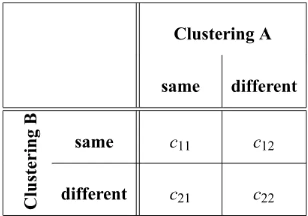
of match between two clusterings, A and B, may be compared by constructing a contingency table

(refer to Figure 1). In this table, c11(c22) is the number of pattern pairs that are in a same (different)

cluster in both partitions. The value c21 is the number of pattern pairs that are placed in a same

cluster by A, but in different clusters by B. The value c12 reflect the converse situation. The four

variables within the contingency table have been used to derive measures of similarity between two clusterings A and B [2] [11]. These measures are known in pattern recognition literature as external criterion indices, and used for evaluating the capacity to recover the true cluster structure.

Table 1: Contingency table used to compare two clusterings. Clustering A same different same c11 c12 Clustering B different c21 c22

Of these measures, the Rand Adjusted [27], define by:

SRA A B 2 c11c22 c12c21

2c11c22 c11 c22 c12 c21 c2₁₂ c2₂₁ (21)

has been selected to assess clustering quality in this paper.

Since correct classificatio results are known for the data sets used, their patterns are all accom-panied by category labels. These labels are withheld from the network under test, but they provide a reference clustering, R, with which a clustering produced by computer simulation, A, may be

compared. In this context, variables c11 and c22 represent the number of pattern pairs which are

properly clustered together and apart, respectively, while c12 and c21 indicate the improperly

clus-tered pairs. Eq. (21) now represents a score, SRA A R , that describes the quality of the clustering

produced by the network. The Rand Adjusted score ranges from 0 to 1, where 0 denotes maximum dissimilarity (worst), and 1 denotes equivalence (best).

5.1.2 Unsupervised competitive learning neural networks

Self-organizing neural networks use unsupervised learning to discover relationships of interest (correlations, categories, etc.) that may exist in the input data [26] [32]. Unsupervised competitive

learning (UCL) [21] [22] [23] [30] [35] [36] refers to a family of self-organizing neural networks, typically applied to adaptive vector quantization [18] [20] [31] for, e.g., data compression, or to discover clusters in unlabeled data [2] [11] [25].

Structurally, a basic UCL neural network consists of a layer of identical output neurons, each one fully connected to the input neurons (one per input feature) with feedforward weights. A category label is associated with each output neuron, and a prototype — the numerical values of the set of weights connecting an output neuron to all input neurons — represents a category’s features. When an input pattern is presented to the network’s input neurons, signals are propagated through the feedforward weight connections, and the output neurons compete among themselves for winner-take-all activation. The output neuron that is active after the competition is the one whose prototype most closely resembles the input pattern. This neuron is declared the winner, its category is assigned to the input, and then it is allowed to adapt its prototype. From a succession of input patterns, output neurons learn to specialize for regions of the input space [26] [35].

An UCL network applied to high throughput category learning for the two types of environ-ments considered in this paper should deliver a rapid category assignment and prototype adap-tation in response to each input pattern. The network’s behavior should also be independent of

the distribution of input patterns among categories1_{. Finally, the network should learn}

incremen-tally, and remain adaptive or plastic to new information which may arise at any time in a non-stationary data stream. Plasticity to new information may cause instability or amnesia in standard UCL networks, since weights can erode over time [23]. Variants such as the Self-Organizing

1_{Independence of behavior to the mixture of patterns assigned to categories precludes the use of a series of UCL}

extensions, such as the Conscience Method [10] [29] and Frequency Sensitive Competitive Learning [1], that apply a conscience principle [21] [22] to overcome an output neuron under-utilization problem.

Feature Map (SOFM) [30] can achieve stability by monotonic reduction of the learning rate and neighborhood function as learning progresses. In contrast, Adaptive Resonance Theory (ART) networks [5] [21] [22] [23] can develop stable recognition capability on-line. They categorize fa-miliar inputs into previously learned adaptive categories, and create new categories dynamically for inputs different enough from those previously seen. Their weights remain stable, yet plastic in response to new events because they can create new categories, while keeping formerly learned weights intact [22]. A vigilance parameter is used to regulate the maximum tolerable difference between any two input patterns to which a category is assigned.

The UCL neural networks selected for computer simulations are (1) standard UCL with Mal-halanobis distance, (2) ART2A-E [15], and (3) fuzzy ART [6]. Networks (1) and (2) are well suited for the firs type of environment (described in Sections 4.4.2), where clusters are explicitly modeled as mean vectors. Networks (2) and (3) are appropriate for the second type of environ-ment, where clusters are modeled implicitly. Appendix A highlights the main architectural and algorithmic characteristics of these three neural networks.

Programs emulating these neural networks were written in the Matlab language for all three data processing schemes. For reordered processing, each network was granted the capacity to de-tect ambiguity. The Gaussian rejection model (refer to Eq. (17) was used in (1) standard UCL and (2) ART2A-E networks. The softmax rejection model (refer to Eq. (20) was used in (3) ART2A-E

and (4) fuzzy ART networks. For standard UCL, j dj, for j 1 2 N, was substituted into

Eq. (20). For ART2A-E or fuzzy ART, j Tj, for j such that the vigilance test is passed was

5.1.3 Data sets

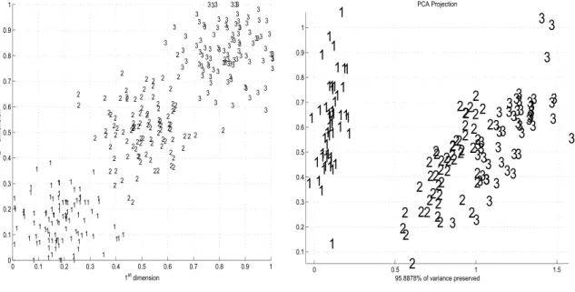
Two data sets were employed: Gaussian and Iris. The Gaussian data set represents the firs type of on-line clustering environment considered in this paper. It is mostly targeted towards clustering systems based on the standard UCL and ART2A-E networks with the Gaussian rejection model. The Iris data set represents the second type of on-line clustering environment. It is targeted towards clustering systems based on the ART2A-E and fuzzy ART networks with the softmax rejection model.

(a) Gaussian data: The Gaussian data set consists of 3 clusters with mean vectors 1 1 1 ,

2 3 3 and 3 5 5 . Each cluster j 1 2 3 is formed by the random generation of 100

patterns from a normal spherical distribution centered at j, with standard deviation 0 6. A

new Gaussian data set was artificiall generated for each simulation trial. Figure 2(a) shows a typical Gaussian data set after normalization.

(b) Iris data: The well-known Iris data set [14] contains parameters from 150 fl wers, each

one belonging to one of three species of iris fl wers — satosa, versicolor and virginica. Fifty fl wers belong to each species, and each fl wer is characterized by its petal and sepal length and width (4 features). Figure 2(b) shows a two-dimensional principal component analysis (PCA) projection of the Iris data set after normalization. Data clusters are scattered, and two of them overlap considerably.

0 0.1 0.2 0.3 0.4 0.5 0.6 0.7 0.8 0.9 1 0 0.1 0.2 0.3 0.4 0.5 0.6 0.7 0.8 0.9 1 1 1 1 1 1 1 1 1 1 1 1 1 1 111 1 1 1 11 1 1 1 11 1 1 1 1 1 1 1 1 ₁ 1 ₁ 1 1 1 1 1 1 1 1 1 ₁ 1 1 1 1 1 1 1 1 1 1 1 1 1 1 1 1 1 1 1 1 1 11 1 1 1 1 1 1 1 1 1 1 1 1 1 1 1 1 1 1 1 1 1 1 1 1 1 1 1 1 1 1 2 2 2 2 2 2 2 2 2 2 2 2 2 2 2 2 2 2 2 2 2 2 2 2 2 2 2 2 2 2 2 2 2 2 2 2 2 ₂2 2 2 2 2 2 2 2 2 2 2 2 2 2 2 2 2 2 2 2 2 2 2 2 2 2 2 2 2 2 2 2 2 2 2 2 2 ₂ 2 2 2 2 2 2 2 2 2 2 2 2 2 2 2₂ 2 2 2 2 2 22 2 3 3 3 3₃ 3 3 3 3 3 3 ₃ 3 3 3 3 ₃ 3 ₃ 3 3 3 3 3 3 3 3 3 3 3 3 ₃₃ 3 3 3 3 3 3 3 3 3 3 3 3 3 3 3 3 3 3 3 3 3 3 3 3 3 3 3 3 3 3 3 3 3 3 3 3 3 3 3 3 3 3 3 3 3 3 3 3 3 3 3 3 3 3 3 3 3 3 3 3 3 3 3 3 3 3 3 1st dimension 2 nd dimension

(a) Gaussian data.

0 0.5 1 1.5 0.1 0.2 0.3 0.4 0.5 0.6 0.7 0.8 0.9 1 1 1 1 1 1 1 11 1 1 1 1 1 1 1 1 1 1 1 1 1 1 1 1 1 1 1 11 11 1 11 1 1 1 1 1 11 1 1 1 1 1 1 1 1 1 2 2 2 2 2 2 2 2 2 2 2 2 2 2 2 2 2 2 2 2 2 2 2 22 2 2 2 2 2 2 2 2 2 2 2 2 2 2 22 2 2 2 2 22 2 2 2 3 3 3 3 3 3 3 3 3 3 3 3 3 3 3 3 3 3 3 3 3 3 3 3 33 3 3 3 3 3 3 3 3 3 3 3 3 3 3 33 3 33 3 3 3 3 3 PCA Projection 95.8878% of variance preserved

(b) PCA projection of the Iris data.

Figure 2: The two data sets used for computer simulations.

5.2 Correlation of ambiguity with clustering quality

The clustering quality achieved by UCL networks is now examined in relation with the degree of ambiguity observed in their category assignments. Patterns from the Gaussian and Iris data sets were categorized by UCL neural networks using reordered processing. Regular network param-eters like the learning rate were fi ed a priori, for each data set, to values that produce a high

Rand Adjusted score SRA A R using sequential processing.

For a same randomly-selected presentation order, the rejection threshold was varied from

trial to trial, in the range from 0 to 1. Patternsa leading to ambiguous category assignments were

detected, yet processed without delay (the mechanism to postpone patterns was deactivated). After

each trial, the score SRA A R , and the empirical rejection rate ˆprwere computed and stored. The

0 0.1 0.2 0.3 0.4 0.5 0.6 0.7 0.8 0.9 1 0

correlation coefficient

rejection threshold ( )

UCL w/ Gaussian rejection fuzzy ART w/ softmax rejection

(a) Gaussian data set.

0 0.1 0.2 0.3 0.4 0.5 0.6 0.7 0.8 0.9 1

0

correlation coefficient

rejection threshold ( )

fuzzy ART w/ softmax rejection

(b) Iris data set.

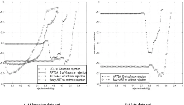
Figure 3: Correlation between the Rand Adjusted score, SRA R A , and the empirical rejection rate,

ˆpr, for three clusterers, two rejection criteria and two data sets. Notice that Iris data simulations

do not apply when UCL networks are augmented with Gaussian rejection, since category spread information ( ) is unavailable.

patterns (the size of the data set). As mentioned in Section 4.3, the number of rejections generally decreases as the threshold is increased. In the context of on-line category learning, the number of rejections varies according to the order in which data are presented. This number also varies with

different random generations of Gaussian data. The linear correlation between scores SRA A R

and respective rates ˆpr was computed from a series of 1000 independent presentation orders, with

ranging from 0 to 1.

The linear correlation coefficient obtained with the Gaussian and Iris data sets are shown in Figure 3(a) and (b), respectively. Table 2 documents the peak negative correlation coefficien

values in Figure 3 for future reference. Results reveal that, for all the clustering systems, and for

both data sets, there is a significan negative correlation between ˆpr and SRA A R . From one trial

to the next, and for a given threshold value , an increase in the number of ambiguous category assignments corresponds to a decline of the clustering score.

The four clustering systems display strong negative correlations, albeit in different ranges of values for the threshold . In simulations involving the Gaussian data, the Gaussian rejection define relatively thin ambiguity regions owing to the explicit use of category spread information

( 2 _{0 36 in Eq. (17)). The conditional error function r}

J a associated with the Gaussian rejection

criterion Eq. (11), which define the ambiguity region, declines relatively quickly at the decision boundary of category J. Consequently, the two UCL networks that use Gaussian rejection achieve

strong negative correlations at low threshold values ( 0 4).

In contrast, softmax rejection does not use category variance information, and thus define

rel-atively wide ambiguity regions. The conditional error function rJ a associated with the softmax

rejection criterion (Eq. (20)) declines relatively slowly at the decision boundary of category J. Fur-thermore, the ART networks have a tendency to create more than three categories to represent the data clusters in Gaussian and Iris sets. Consequently, ART2A-E achieves strong negative

correla-tions at high threshold values ( 0 55 0 70 ) for both data sets. It is interesting to note that,

despite making abstraction of information, softmax rejection can provide a negative correlation almost equivalent in strength to that obtained with Gaussian rejection.

Table 2: Peak ne gati ve correlation coef ficien values associated with Figure 3. The rejection threshold value ,empirical rejection rate ˆpr (with standard error in parentheses) and parameter settings that correspond to these peak correlations are also sho wn.

Corr

elation

Coefficien

Neural

Netw

orks

Fuzzy ART using the softmax rejection model displays strong negative correlation across a wide range of threshold values. Its ability to assess ambiguity appears less sensitive to input data structure, as it provides consistently strong negative correlations for both data sets. This can be explained by the fact that fuzzy ART is the most susceptible of the three UCL networks to ambiguity. Indeed, fuzzy ART is unable to forget, and hence recover from category miss-assignments.

5.3 Clustering quality obtained using reordered processing

Having shown that the Gaussian and softmax rejection models detect ambiguous category assign-ments, and that these assignments lead to poor clustering performance, the effect of delaying such assignments is now examined.

For a same randomly-selected presentation order, the rejection threshold was varied from 0 to 1, over successive trials. During each trial, patterns from either the Gaussian or Iris data set were presented to a clustering system used with reordered processing. As in Subsection 4.5.2,

the network parameters were fi ed a priori to provide high Rand Adjusted scores SRA R A using

sequential processing. Rejected patterns were delayed by d patterns. Two different delay values,

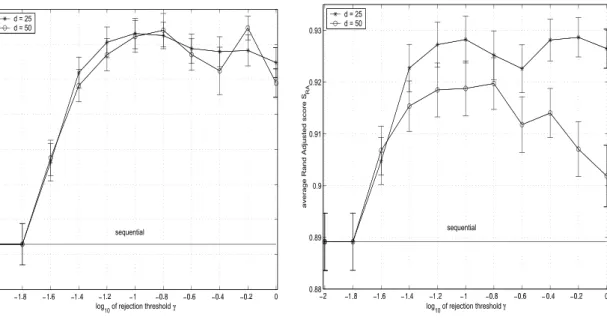
d 25 and 50, were tried. After each trial, the score, SRA A R and empirical rejection rate, ˆpr,

were computed and stored. Average SRA A R and ˆpr values were obtained from a series of 20

independent presentation orders, with ranging from 0 to 1.

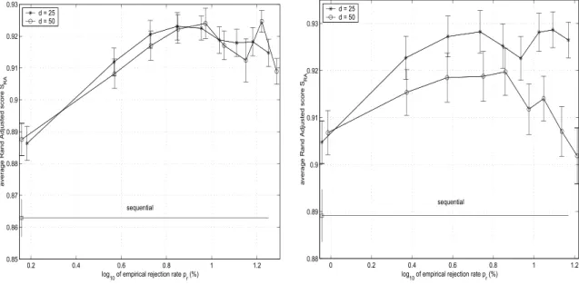
Figure 4 shows the average SRA A R as a function of for four different cases — standard UCL

and ART2A-E on Gaussian data, and ART2A-E and fuzzy ART on Iris data. Figure 5 shows the

0 0.85 0.86 0.87 0.88 0.89 0.9 0.91 0.92 0.93

log₁₀ of rejection threshold

average Rand Adjusted score S

RA

d = 25 d = 50

sequential

(a) standard UCL on Gaussian data.

0 0.88 0.89 0.9 0.91 0.92 0.93

log₁₀ of rejection threshold

average Rand Adjusted score S

RA

d = 25 d = 50

sequential

(b) ART2A-E on Gaussian data.

0 0.1 0.2 0.3 0.4 0.5 0.6 0.7 0.8 0.9 1 0.6 0.61 0.62 0.63 0.64 0.65 0.66 rejection threshold

average Rand Adjusted score S

RA

d = 25 d = 50

sequential

(c) ART2A-E on Iris data.

0 0.1 0.2 0.3 0.4 0.5 0.6 0.7 0.8 0.9 1 0.46 0.47 0.48 0.49 0.5 0.51 0.52 0.53 0.54 0.55 rejection threshold

average Rand Adjusted score S

RA

d = 25 d = 50

sequential

(d) fuzzy ART on Iris data.

Figure 4: Average Rand Adjusted scores SRA A R versus rejection threshold for simulations

0.2 0.4 0.6 0.8 1 1.2 0.85 0.86 0.87 0.88 0.89 0.9 0.91 0.92 0.93

log₁₀ of empirical rejection rate p_r (%)

average Rand Adjusted score S

RA

d = 25 d = 50

sequential

(a) standard UCL on Gaussian data.

0 0.2 0.4 0.6 0.8 1 1.2 0.88 0.89 0.9 0.91 0.92 0.93

log₁₀ of empirical rejection rate p_r (%)

average Rand Adjusted score S

RA

d = 25 d = 50

sequential

(b) ART2A-E on Gaussian data.

0 5 10 15 20 25 30 35 40 0.6 0.61 0.62 0.63 0.64 0.65 0.66

empirical rejection rate p_r (%)

average Rand Adjusted score S

RA

d = 25 d = 50

sequential

(c) ART2A-E on Iris data.

0 10 20 30 40 50 0.46 0.47 0.48 0.49 0.5 0.51 0.52 0.53 0.54 0.55

empirical rejection rate p_r (%)

average Rand Adjusted score S

RA

d = 25 d = 50

sequential

(d) fuzzy ART on Iris data.

Figure 5: Average Rand Adjusted scores SRA A R versus empirical rejection rate ˆpr for

simula-tions with Gaussian and Iris data. (Error bars are standard error.) The standard error for values of

the clustering score significantlyover sequential processing alone. For example, if pattems from

theIris dataare presentedtotheclusteringsystem withfuzzy ARTand d = 50,thenreordered

sequential processing improves the score Sm(A,R) by about 13%. Clustering improvements are

achieved over a wide range of y values. Inthe example given above (fuzzy ART onthe Iris data),

the maximum score ofSM(A,R) 2 0.538is obtained fory~ [0.5,0.8], correspondingtoPr g 55%

in Figure 5. For 0 2 y < 0.5, the performance tends towards that of sequential processing since

Pr + 0%. With y > 0.8,the performance also tendsto decline because ofthelarge number of

rejections. Noticethatimprovementsto SM (A, R)occur when there is a strong negative cor-relation

between Pr andSu (A, R).

Ofthefourcases,reordered processingappears most beneficialtoaclusteringsystem with

fuzzy ART, where irreversible leaming has the strongest impact. TOensure stability, fuzzy ART

weights are adjusted such thateach category hyperrectanglecan only grow or remainthesame. In

contrast, standard UCL andART2A-E representcategories asmean vectors, and obtaintheir best

performance at slower leaming rates, which allow to “forget” some category miss-assignments due

to ambiguity.

5.4 C

luster

ing qua

l

ity and

latency

For fast on-line clustering applications, the quality of results must be balanced with the response

time needed to produce the results. The performance of different clustering systems is now

com-paredinterms of clustering quality andlatency.

Fora same randomly-selected presentation order, the queue lengths k and d were varied

be-tween 5 pattems and halfthe number of pattemsinthe data set, over successivetrials. This range

guarantees at least two batches of k patterns for batch processing, and limits the amount of pat-terns being postponed at any given time for reordered processing. During each trial, patpat-terns from either the Gaussian or Iris data set were presented to the batch and reordered processing architec-tures. With the batch processing architecture, the UCL network was left to converge for successive batches of k patterns, until prototype weights were identical for two consecutive epochs. Regular

network parameters were fi ed a priori to provide high Rand Adjusted scores SRA R A with batch

processing when k is one half the data set size. With the reordered processing architecture, a dif-ferent rejection threshold value was selected for each UCL network. Regular network parameters

were fi ed a priori to provide high scores SRA R A with sequential processing. Rejected input

patterns were delayed for d patterns. After each trial, the score SRA R A , the lower bound on the

average latency L (Eq. (3)), and the average latency L of the considered architectures (Eq. (7) for

the batch case) were computed. The empirical rejection rate, ˆpr, provides a fi ed estimate of the

variable rejection rate pr a , and was substituted into Eq. (3). Simulations were repeated 20 times

for every k and d value in order to yield representative results.

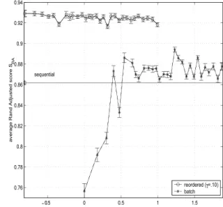
The average scores SRA A R as a function of the lower bounds on average latency L are shown

in Figure 6 for four different cases — standard UCL and E on Gaussian data, and ART2A-E and fuzzy ART on Iris data. Both batch and reordered processing achieve significantl higher scores than sequential processing. However, reordered processing achieves the improvement at a much lower average latency than batch processing. For example, with fuzzy ART on the Iris data,

reordered processing with 0 65 yields a score of SRA A R 0 534 for an average latency of

L 6 4 patterns. This corresponds to ˆpr 42 5% and d 15. By comparison, batch processing

0 0.5 1 1.5 0.74 0.76 0.78 0.8 0.82 0.84 0.86 0.88 0.9 0.92 0.94

log₁₀ of the lower bound on average latency L (patterns)

average Rand Adjusted score S

RA

reordered ( =.10) batch sequential

(a) standard UCL on Gaussian data.

0 0.5 1 1.5 0.76 0.78 0.8 0.82 0.84 0.86 0.88 0.9 0.92 0.94

log₁₀ of the lower bound on average latency L (patterns)

average Rand Adjusted score S

RA

reordered ( =.10) batch sequential

(b) ART2A-E on Gaussian data.

0 5 10 15 20 25 30 35 0.54 0.56 0.58 0.6 0.62 0.64

lower bound on average latency L (patterns)

average Rand Adjusted score S

RA

reordered ( =.50) batch sequential

(c) ART2A-E on Iris data.

0 5 10 15 20 25 30 35 0.44 0.46 0.48 0.5 0.52 0.54 0.56

lower bound on average latency L (patterns)

average Rand Adjusted score S

RA

reordered ( =.65) batch sequential

(d) fuzzy ART on Iris data.

Figure 6: Average Rand Adjusted scores SRA A R versus lower bound on average latency L for

0 0.5 1 1.5 2 0.74 0.76 0.78 0.8 0.82 0.84 0.86 0.88 0.9 0.92 0.94

log₁₀ of lower bound on average latency L (patterns)

average Rand Adjusted score S

RA

reordered architecture ( =.10) batch architecture sequential

(a) standard UCL on Gaussian data.

0 0.5 1 1.5 2 0.76 0.78 0.8 0.82 0.84 0.86 0.88 0.9 0.92 0.94

log₁₀ of lower bound on average latency L (patterns)

average Rand Adjusted score S

RA

reordered architecture ( =.10) batch architecture sequential

(b) ART2A-E on Gaussian data.

0 10 20 30 40 50 60 70 80 90 100 0.54 0.56 0.58 0.6 0.62 0.64

lower bound on average latency L (patterns)

average Rand Adjusted score S

RA

reordered architecture ( =.50) batch architecture sequential

(c) ART2A-E on Iris data.

0 20 40 60 80 100 0.44 0.46 0.48 0.5 0.52 0.54 0.56

lower bound on average latency L (patterns)

average Rand Adjusted score S

RA

reordered architecture ( =.65) batch architecture sequential

(d) fuzzy ART on Iris data.

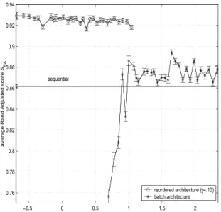
Figure 7: Average Rand Adjusted scores SRA A R versus average latency L of the batch and

Results in Figure 6 reveal that the performance obtained with batch processing increases with

k until a peak value. Peak performance with reordered processing sometimes exceed that of batch

processing. It often occurs for relatively small values of d, indicating that it is suitable for high speed applications. Beyond this peak, increasing d does not necessarily deliver a greater score

SRA A R . This is due to our emulation of an infinit data stream with a fi ed-sized data set. If an

inputa to be processed is among the last d patterns of a data set, and it is rejected by the clusterer,

then it is postponed to the end of the data set (following any other previously-rejected patterns),

and may be postponed for less than d patterns. Asa is located closer to the end of the data set, and

as and d grow, it is more likely fora to be postponed by less than d patterns. Clustering quality

accordingly converges towards that of sequential processing.

The average scores SRA A R as a function of the average latency L for the batch and reordered

architectures are shown in Figure 7. With the batch architecture, there is a substantial difference between the curves obtained with L and those obtained with the lower bound on L. Indeed, using the batch processing architecture requires between 2 and 5 epochs for convergence on each batch of patterns. Assuming that the techniques used to assess ambiguity have a relatively low computa-tional complexity, the average latency of the reordered architecture compares favorably to that of the batch architecture.

6 Conclusions

Both clustering quality and response time are critical in many on-line category learning applica-tions. A clustering system targeted for high throughput applications would traditionally consist of a clusterer that processes input patterns sequentially. Despite the fast response time obtained when

using this data processing scheme, the quality and consistency of the results remain an issue. By contrast, batch processing yields higher clustering quality, but incurs longer delays.

In this paper, an alternative called reordered processing has been presented. It consists in post-poning for a fi ed time the learning of patterns for which category assignments are ambiguous. Ambiguity occurs when the clusterer lacks the information needed to take a fir decision in fa-vor of a single category. The reject option from statistical pattern recognition literature has been extended for the detection of ambiguous category assignments. Reordered processing alters the original pattern presentation order in an attempt to avoid ambiguous decisions. In addition, it pro-vides control of the maximum response time of a clustering system. Latency of on-line category learning has been define and used to compare sequential, batch or reordered processing. In order to reveal some of the practical considerations of implementing batch and reordered processing, the latency of two high level architectures have also been described.

Computer simulations were performed by presenting patterns from two data sets to several neural networks with sequential, batch and reordered processing. Results of these simulations indicate that (1) the number of category assignments detected as ambiguous is correlated with poor clustering quality; (2) reordered processing improves clustering quality over sequential processing alone and sometimes over batch processing; and (3) it offers an interesting alternative to batch processing in terms of trading off clustering quality for response time.

Acknowledgements

This research was supported in part by the Fonds pour la Formation de Chercheurs et l’Aide `a la Recherche du Qu´ebec, and the Natural Sciences and Engineering Research Council of Canada.

References

[1] Ahalt, S. C., Krishnamurthy, A. K., Chen, P., and Melton, D. E., “Competitive Learning

Algorithms for Vector Quantization,” Neural Networks,3, 277-290, 1990.

[2] Anderberg, M. R., Cluster Analysis for Applications, London, UK: Academic Press, 1973. [3] Bishop, C., Neural Networks for Pattern Recognition, Oxford, UK: Clarendon Press, 1995. [4] Bridle, J. S., “Probabilistic Interpretation of Feedforward Classificatio Network Outputs,

with Relationships to Statistical Pattern Recognition,” in Neurocomputing – Algorithms,

Ar-chitectures and Applications, eds., Fogelman-Souli´e, F., H´erault, J., NATO ASI Series F68,

Berlin: Springer-Verlag, 227-236, 1989.

[5] Carpenter, G. A. and Grossberg, S., “A Massively Parallel Architecture for a Self-Organizing Neural Pattern Recognition Machine,” Computer, Vision, Graphics and Image Processing,

37, 54-115, 1987.

[6] Carpenter, G. A., Grossberg, S., and Rosen, D. B., “Fuzzy ART: Fast Stable Learning and

Categorization of Analog Patterns by an Adaptive Resonance System,” Neural Networks,4:6,

759-771, 1991.

[7] Chow, C. K., “An Optimum Character Recognition System Using Decision Functions,” IRE

Trans. Electronic Computers,6, 247-254, 1957.

[8] Chow, C. K., “On Optimum Recognition Error and Reject Tradeoff,” IEEE Trans.

[9] Davies, C. L. and Hollands, P., “Automatic Processing for ESM,” Proc. IEE,129:3 (F),

164-171, June 1982.

[10] DeSieno, D., “Adding a Conscience to Competitive Learning,” Proc. IEEE Int’l Conf. Neural

Networks, 1117-1124, San Diego, June 1988.

[11] Dubes, R. C. and Jain, A. K., Algorithms for Clustering Data, Englewood Cliffs, NJ:Prentice Hall, 1988.

[12] Dubuisson, B. and Masson, M., “A Statistical Decison Rule with Incomplete Knowledge

About Classes,” Pattern Recognition,26:1, 155-165, 1993.

[13] Duda, R. O., and Hart, P. E., Pattern Classificatio and Scene Analysis, John Weiley & Sons, 1973.

[14] Fisher, R. A., “The Use of Multiple Measurements in Taxonomic Problems,” Annals of

Eu-genics,7, 1936.

[15] Frank, T., Kraiss, K.-F., and Kuhlan, T., “Comparative Analysis of Fuzzy ART and ART-2A

Network Clustering Performance,” IEEE Trans. Neural Networks,9:3, 544-559, 1998.

[16] Fukunaga, K. and Kessell, D. L., “Application of Optimal Error-Reject Functions,” IEEE

Trans. Information Theory, 814-817, November 1972.

[17] K. Fukunaga, Introduction to Statistical Pattern Recognition, Academic Press, 2nd ed., 1990.

[18] Gersho, A., “On the Structure of Vector Quantizers,” IEEE Trans. Information Theory,28:2,

[19] Granger, E., Savaria, Y., Lavoie P., and Cantin, M.-A., “A Comparison of Self-Organizing

Neural Networks for Fast Clustering of Radar Pulses,” Signal Processing, 64:3, 249-269,

1998.

[20] Gray, R. M., “Vector Quantization,” IEEE ASSP Magazine,1:2, 4-29, 1984.

[21] Grossberg, S., “Adaptive Pattern Classificatio and Universal Recoding: I. Parallel

Develop-ment and Coding of Neural Detectors,” Biological Cybernetics,23, 121-134, 1976.

[22] Grossberg, S., “Adaptive Pattern Classificatio and Universal Recoding: II. Feedback,

Oscil-lation, Olfaction, and Illusions,” Biological Cybernetics,23, 187-207, 1976.

[23] Grossberg, S., “Competitive Learning: From Interactive Activation to Adaptive Resonance,”

Cognitive Science,11, 23-63, 1987.

[24] Ha, T. M., “The Optimal Class-Selective Rejection Rule,” IEEE Trans. Pattern Analysis and

Machine Intelligence,19:6, 608-615, 1997.

[25] Hartigan, J. A., Clustering Algorithms, New York, NY: Wiley, 1975.

[26] Haykin, S., Neural Networks: A Comprehensive Foundation, Macmillan College Press, 1994.

[27] Hubert, L. and Arabie, P., “Comparing Partitions,” Journal of Classificatio , 2, 193-218,

1985.

[28] Hellman, M. E., “The Nearest Neighbor Classificatio Rule with Reject Option,” IEEE Trans.

Systems Science and Cybernetics,6:3, 179-185, 1970.

[29] Hecht-Nielsen, R., “Applications of Counterpropagation Networks,” Neural Networks, 1,

[30] Kohonen, T., Self-Organization and Associative Memory, Springer-Verlag, 3rd ed., 1989. [31] Linde, Y., Buzo, A., and Gray, R. M., “An Algorithm for Vector Quantizer Design,” IEEE

Trans. Communications,28:1, 84-95, 1980.

[32] Lin, C.-T. and George Lee, C. S., Neural Fuzzy Systems: A Neuro-fuzzy Synergism to

Intelli-gent Systems, Prentice-Hall, 1995.

[33] Lloyd, S. P., “Least-square Quantization in PCM,” IEEE Trans. Information Theory, 28:2,

129-137, 1982.

[34] MacQueen, J., “Some Methods for Classificatio Analysis of Multivariate Observations,”

Proc. 5th Berkley Symposium on Mathematical Statistics and Probability, 281-297, 1967.

[35] Rumelhart, D. E. and Zipser, D., “Feature Discovery by Competitive Learning,” Cognitive

Science,9, 75-112, 1985.

[36] Von der Malsberg, C., “Self-Organizating of Orientation Sensitive Cells of the Striate

A Summary of UCL neural networks

A.1 Neural network structure

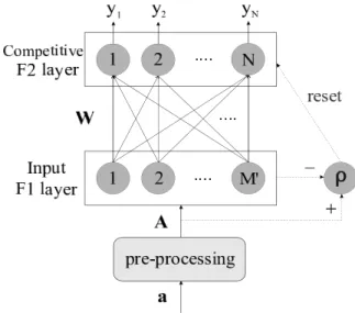
A simplifie UCL neural network (refer to Figure 8) consists of two layers of neurons that are fully

connected: an M neuron input layer, F1, and an N neuron output or competitive layer, F2. Each

F1neuron i is associated with an input feature, whereas every F2neuron j represents a category in

the input space. A set of adaptive weightsW wi j : i 1 2 M; j 1 2 N is associated

with the F1-to-F2layer connections. Weight value wi j is represented as a real in the interval [0,1].

Finally, as shown in the shaded parts of Figure 8, ART networks also require circuitry to perform vigilance testing (refer to Section 4.A.2).

For each neuron j of F2, the prototype wj w1 j w2 j wM j define the characteristics of

category j. With standard UCL and ART2A-E networks, each prototype represents a center point in the input scene (computed from patterns assigned to that category). In this respect, fuzzy ART differs significantl from the other two, since prototype vectors represent fuzzy set hyperrectangles.

A.2 Algorithmic description

Neural network processing can be define in terms of algorithmic steps. The following algorithm describes the operation of the UCL networks in general terms. Table 3 provides the specifi equa-tions that extend this general description to the standard UCL with Malhalobis distance, ART2A-E and fuzzy ART networks.

1. Weights and parameters initialization: An F2 neuron j is labeled as committed after being

assigned to an m-dimensional input patterna a1 a2 am . With standard UCL networks, a

fi ed number N of F2 neurons is committed in advance. Respective prototypes wj are preset to

the value of N randomly-selected input vectorsa. With ART networks, all F2neurons are initially

uncommitted, but the number of committed F2neurons grows progressively. The learning rate ,

vigilance and choice parameters are define at this step.

2. Input preprocessing: When a new input vector a is presented to the network, it may undergo

a preliminary coding, such as normalization. With fuzzy ART, a transformation called complement

coding doubles the number of components in the input pattern (M 2m), which becomes A = a;ac _{= a1 a2 am;a}c

1 ac2 acm , where aci 1 ai . With complement coding, fuzzy ART

represents category j as a hyperrectangle that just encloses the training set patternsa to which it

has been assigned. That is, a M-dimensional prototypewj w1 j w2 j wM j records the largest

and smallest component values of training set patternsa placed in the jth category.

3. Category assignment: Input pattern A activates layer F1and is propagated through weighted

choice function. The F2layer produces a binary, winner-take-all pattern of activityy y1 y2 yN ,

where only the neuron j J with the greatest activation value remains active (yJ 1). If the

great-est activation value is obtained by two or more neurons, the one with the smallgreat-est index j wins. In addition, the winning neuron J is subjected to a vigilance test in ART networks. If this test is passed, then neuron J remains active and resonance occurs. Otherwise, the network inhibits the

active F2neuron and searches for another neuron J that passes the vigilance test. If such a neuron

does not exist, an uncommitted F2neuron becomes active and undergoes prototype update.

4. Prototype learning: The prototype wJof the winning neuron J is adjusted to account for input A. The algorithm can be set to slow learning, with 0 1, or to fast learning, with 1. Once prototype update is performed, the network is ready to process another input pattern (at Step 2).

Table 3: Distincti ve equations used by standard UCL, AR T2A-E and fuzzy AR T netw orks. Operator is the L1 norm, wj M i1 wij ,whereas is the Euclidean distance or L2 norm, A wj M i1 Ai wji 2.W ith fuzzy AR T, is the fuzzy AND operator , A wj i min Ai wij .

Neural

Netw

ork

Algorithmic

Step