DOI:10.1051/0004-6361/201526983
c
ESO 2016
Astrophysics
&
Radiative rates for forbidden M1 and E2 transitions
of astrophysical interest in doubly ionized iron-peak elements
V. Fivet
1, P. Quinet
1,2, and M. A. Bautista
31 Physique Atomique et Astrophysique, Université de Mons – UMONS, 7000 Mons, Belgium e-mail: vanessa.fivet@gmail.com
2 IPNAS, Université de Liège, 4000 Liège, Belgium
3 Department of Physics, Western Michigan University, Kalamazoo, MI 49008, USA
Received 17 July 2015/ Accepted 11 September 2015
ABSTRACT
Aims.Accurate and reliable atomic data for lowly ionized Fe-peak species (Sc, Ti, V, Cr, Mn, Fe, Co, and Ni) are of paramount impor-tance for analyzing the high-resolution astrophysical spectra currently available. The third spectra of several iron group elements have been observed in different galactic sources, such as Herbig-Haro objects in the Orion Nebula and stars like Eta Carinae. However, for-bidden M1 and E2 transitions between low-lying metastable levels of doubly charged iron-peak ions have been investigated very little so far, and radiative rates for those lines remain sparse or nonexistent. We attempt to fill that gap and provide transition probabilities for the most important forbidden lines of all doubly ionized iron-peak elements.
Methods.We carried out a systematic study of the electronic structure of doubly ionized Fe-peak species. The magnetic dipole (M1) and electric quadrupole (E2) transition probabilities were computed using the pseudo-relativistic Hartree-Fock (HFR) code of Cowan and the central Thomas-Fermi-Dirac-Amaldi potential approximation implemented in AUTOSTRUCTURE. This multiplatform ap-proach allowed for consistency checks and intercomparison and has proven very useful in many previous works for estimating the uncertainties affecting the radiative data.
Results.We present transition probabilities for the M1 and E2 forbidden lines depopulating the metastable even levels belonging to the 3dkand 3dk−14s configurations in Sc III (k= 1), Ti III (k = 2), V III (k = 3), Cr III (k = 4), Mn III (k = 5), Fe III (k = 6), Co III (k= 7), and Ni III (k = 8).
Key words.atomic data – atomic processes
1. Introduction
In relation to their high cosmic abundance, accurate and reli-able atomic data for the iron-peak elements are crucial in as-trophysics. The advent of high-resolution astrophysical spec-troscopy has led to observing these elements in low-ionization stages in various astronomical objects. Emission lines of dou-bly ionized Fe-peak species have been observed in several nebular environments. Recent Hubble Space Telescope/Space Telescope Imaging Spectograph (HST/STIS) observations from the Weigelt blobs of Eta Carinae (η Car) have revealed several forbidden lines of Fe III and Ni III (Zethson et al. 2012). Lines of doubly ionized species have also been detected in various galac-tic sources, such as Herbig-Haro objects in the Orion Nebula (Mesa-Delgado et al. 2009) and extragalactic objects, includ-ing active galactic nuclei (Vestergaard & Wilkes 2001). Reliable radiative data are therefore essential for interpreting these ob-servations and obtaining a diagnostic of the physical conditions in the astrophysical plasma. However, our knowledge of doubly charged iron-peak ions is still incomplete, in particular when it comes to forbidden transitions between the low-lying metastable states.
Atomic data calculations for iron-peak elements are very challenging owing to the complexity of these systems due to the open 3d subshell. In particular, transition probabilities for mag-netic dipole (M1) and electric quadrupole (E2) lines are very
difficult to compute due to their extreme sensitivity to config-uration interaction and level mixing. Forbidden radiative rates were only available for selected transitions in five ions of the doubly ionized Fe peak. As the simplest atomic structure con-sidered in this work, doubly ionized scandium has been investi-gated extensively byAli & Kim(1988) using the multiconfigura-tional Dirac-Fock (MCDF) method, byZeippen(1990) with the SUPERSTRUCTURE code, and more recently bySahoo et al. (2008) andNandy et al. (2011), both using an all-order, per-turbative, relativistic many-body approach, i.e. the relativistic coupled-cluster (RCC) method.
Biémont et al.(1992) published a list of ab initio transition probabilities of M1 and E2 transitions within the 3d2 configura-tion of Ti III using the Relativistic Hatree-Fock (HFR) approach and the SUPERSTRUCTURE code.Raassen & Uylings(1997) also performed fully-relativistic multiconfiguration Dirac-Fock (MCDF) calculations for all the metastable levels of this ion. Irimia (2007) published theoretical lifetimes for the 33 lev-els belonging to the low-lying metastable terms of V III us-ing the multiconfiguration Hartree-Fock (MCHF) method with Breit-Pauli (BP) corrections to a non-relativistic Hamiltonian. Selected transition probabilities were also presented in this pa-per. Radiative rates have been computed for the astrophysically important Fe III ion byQuinet(1996) using the HFR approach, byDeb & Hibbert(2009) with the CIV3 code, and more recently byBautista et al.(2010) using the same theoretical methods as
Table 1. Scaling parameters of the Thomas-Fermi-Dirac-Amaldi potential for all the doubly-ionized iron-peak ions considered in this work.
λnl Sc III Ti III V III Cr III Mn III Fe III Co III Ni III
1s, 2s, 2p, 3s and 3p 1.1012 1.0980 1.0867 1.0729 1.0607 1.0350 1.0604 1.0107 3d 1.0908 1.1062 1.1019 1.0912 1.0814 1.0562 1.0190 1.0300 4s 1.1221 1.1115 1.0818 1.0688 1.0533 1.0629 1.1045 1.0342 4p 1.0995 1.1070 1.1040 1.0933 1.0755 1.0511 1.0651 1.0273 4d 1.0905 1.0603 1.1253 1.1084 1.1828 1.0986 1.1420 1.0948 5s 1.1483 1.2782 1.7940 1.7839 1.7728 1.0517 1.6776 1.0384
those presented in this work. Transition rates have also been published for forbidden lines in the 3d7ground configuration of Co III byHansen et al.(1984) using a parametric approach.
When computing forbidden radiative rates, it is common to assess the quality of the results by comparing them with a few metastable lifetime measurements performed with a storage ring (see, e.g.,Lundin et al. 2007). When experimental data are miss-ing, information on the accuracy of the radiative rates can be obtained by comparing calculations using different independent theoretical approaches. The agreement observed between the sets of results allows us to perform consistency checks and es-timate the uncertainties affecting the data. This is the approach adopted in the present work for computing E2 and M1 transi-tion probabilities where we compare the results of two di ffer-ent theoretical methods with each other, together with previous results when available. Since the odd levels can be de-excited by E1 transitions (several orders of magnitude stronger than E2 and M1 transitions) to the even states, odd-odd forbidden transi-tions are of little or no interest because they are very unlikely to be observed in an experimental and/or astrophysical spectrum. Therefore, we chose to limit our work to the even metastable states.
2. Theoretical models
The first theoretical approach used in this work is the pseudo-relativistic Hartree-Fock (HFR) method implemented in Cowan’s chain of computer codes (Cowan 1981). In our calcula-tions, configuration interactions were considered by including the configurations of the type 3dk, 3dk−14s, 3dk−15s, 3dk−14d, 3dk−24s2, 3dk−24p2, 3dk−24d2, 3dk−24s4d, 3dk−24s5s, 3s3p63dk+1,
3s3p63dk4s, and 3s3p63dk−14s2with k= 1 (Sc III), k = 2 (Ti III), k= 3 (V III), k = 4 (Cr III), k = 5 (Mn III), k = 6 (Fe III), k = 7 (Co III), and k = 8 (Ni III). This method was then combined with a least-squares optimization routine that minimizes the dif-ferences between the calculated and available experimental en-ergy levels belonging to the low-lying even configurations 3dk
and 3dk−14s. For Sc III, Ti III, V III, Mn III, Co III, and Ni III, the
experimental data used in this semi-empirical process were taken from the NIST compilation (Kramida et al. 2013), which is ex-clusively based on the previous compilation bySugar & Corliss (1985).
For Cr III and Fe III, we used more recent data fromEkberg (1997) and Ekberg(1993), respectively. We also calculated ra-diative transition rates for M1 and E2 forbidden transitions using the atomic structure code AUTOSTRUCTURE (Badnell 1988). This code is based on the program SUPERSTRUCTURE orig-inally developed by Eissner et al.(1974). In this approach the wavefunctions are written as a configuration interaction expan-sion of the type
ψi=
X
cjiφi, (1)
where the coefficients cji are chosen so as to diagonalize
hψj| H |ψii, where H is the Breit-Pauli Hamiltonian and the
ba-sic functions φjare constructed from one-electron orbitals
gen-erated using the Thomas-Fermi-Dirac-Amaldi model potential (Eissner & Nussbaumer 1969).
The Breit-Pauli Hamiltonian for an N-electron system is given by
Hbp= Hnr+ H1b+ H2b (2)
where Hnris the usual non-relativistic Hamiltonian, and H1band
H2bare the one-body and two-body operators. The one-body
rel-ativistic operator H1b= N X n=1 fn(mass)+ fn(d)+ fn(SO) (3)
represents the spin-orbit interaction fn(SO), the non-fine
struc-ture mass variation fn(mass), and the one-body Darwin fn(d)
corrections. The two-body corrections H2b=
X
n>m
gnm(SO)+ gnm(SS)+ gnm(CSS)+ gnm(d)+ gnm(OO),
(4) usually referred to as the Breit interaction, include, on one hand, the fine-structure terms gnm(SO) (spin-other-orbit and mutual
spin-orbit) and gnm(SS) (spin-spin). On the other hand, they
inclue the non-fine structure terms: gnm(CSS) (spin-spin
con-tact), gnm(d) (Darwin), and gnm(OO) (orbit-orbit). The scaling
parameters λnlfor each nl orbital are optimized by minimizing a
weighted sum of the energies for all the metastable terms belong-ing to the 3dkand 3dk−14s configurations. Instead of optimizing each scaling parameter individually, we chose to optimize the core orbitals 1s, 2s, 2p, 3s, and 3p together to simulate the effect of missing open-core configurations in our model. Table1gives the values of the λnlfor all the ions considered in this work.
The set of configurations used in the AUTOSTRUCTURE model is the same as the one used for the HFR calculations with the addition of 3dk−14p and 3dk−24s4p to ensure a better repre-sentation of the 4p orbital. Semi-empirical corrections take the form of term energy corrections (TEC). By considering the rela-tivistic wavefunction,ψr
i in a perturbation expansion of the
non-relativistic functions ψnri ψr i = ψ nr i + X j,i ψnr i + hψnr j| H1b+ H2b|ψ nr i i Enri − Enrj (5)
where H1b and H2b are, respectively, the one- and two-body
parts of both fine-structure and non-fine-structure Hamiltonians. A modified non-relativistic Hamiltonian is constructed with im-proved estimates of the differences Enr
i − E nr
j so as to adjust
the centers of gravity of the spectroscopic terms to the avail-able experimental values. Term energy corrections (TEC) have
V. Fivet et al.: Radiative rates for forbidden transitions in doubly ionized iron-peak elements
been applied to all the metastable terms considered in this work. TablesA.1toA.8compare, respectively, the level energies (in cm−1), which were obtained before applying the TEC, for all the metastable levels of Sc III, Ti III, VIII, Cr III, Mn III, Fe III, Co III, and Ni III along with the corresponding TEC. The aver-age TEC along the sequence are about 10% or less of the cal-culated energies. For the manganese ion, we were not able to apply TEC to all the metastable terms because this resulted in a switch in the energies and an incorrect representation of the ground state. Therefore, we kept the ab initio term energies for the 3d5c2D1, 3d4(3D)4s c4D, and 3d4(1S2)4s b2S.
3. Forbidden M1 and E2 transition probabilities
In this section, we discuss the radiative data calculations for each ion considered in this work. Transition probabilities can be found in TablesA.9toA.17for all the forbidden lines depopu-lating the metastable levels belonging to the 3dkand the 3dk−14s
configurations. The lack of space means that only the total A-values (M1+E2) contributing more than 10% to the total de-excitation of each level are presented here. The weakest tran-sition probabilities are available upon request to the authors.
3.1. Scandium (Z = 21)
Only three metastable levels arise from 3d and 4s configurations in Sc III. This gives three spectral lines for which we computed the magnetic dipole (M1) and electric quadrupole (E2) contribu-tions. In TableA.9, our HFR and AUTOSTRUCTURE results are compared to the calculations previously published byAli & Kim (1988),Zeippen (1990),Sahoo et al. (2008), and Nandy et al.(2011). As seen from this table, the agreement between all sets of data is excellent (within 10%).
3.2. Titanium (Z = 22)
In TableA.10and Fig.1, we compare our present HFR transi-tion probabilities for M1 and E2 lines involving the levels of 3d2
and 3d4s configurations in Ti III with our AUTOSTRUCTURE results and the previous data published by Biémont et al. (1992) and Raassen & Uylings (1997). Very good agreement (within 5%) is observed between our HFR radiative rates and the MCDF results fromRaassen & Uylings(1997). We also note that our present AUTOSTRUCTURE calculations agree within 15% with both our HFR and Raassen & Uylings’ results for tran-sitions with A values greater than 10−2 s−1, such as 3d2 3F
3–
3d2 1G
4 (λ = 703.55 nm), 3d2 3F4–3d2 1G4 (λ = 715.33 nm),
3d2 3F2–3d2 1D2 (λ = 1180.65 nm), and 3d2 3F3–3d2 1D2
(λ= 1206.31 nm). Despite a systematic discrepancy between the SUPERSTRUCTURE transition probabilities ofBiémont et al. (1992) and all the other sets of results, the overall agreement is still reasonable (within 25%).
3.3. Vanadium (Z = 23)
Computed transition probabilities as obtained in the present work for forbidden lines arising from 3d3 and 3d24s
configu-rations in V III are reported in Table A.11 and compared in Fig.2. We can see that our HFR and AUTOSTRUCTURE data are in excellent agreement (within 5%) for the strongest tran-sitions, while larger discrepancies are observed for some weak lines, in particular for those depopulating the 3d3 2G,2P, 2D2, and2H terms. When comparing the lifetimes of the eight
lev-els corresponding to the last terms (see TableA.12), we find an
O th e r A -v al u e s (s -1) 0 10 20 30 40 50 0 10 20 30 40 50 HFR A-values (s-1) 0 10 20 30 40 50 0 10 20 30 40 50 AUTOS present SST Biémont et al. 1992 MCDF Raassen & Uylings 1997
Fig. 1. Comparison between our present HFR and AUTOS
calcula-tions with the previous results of Biémont et al. (1992) and Raassen & Uylings (1997) for forbidden transitions in Ti III. The straight line of equality has been drawn, and the two dashed lines represent a 10% deviation from equality.
A U T O S A -v al u e s (s -1) 0 20 40 60 80 100 0 20 40 60 80 100 HFR A-values (s-1) 0 20 40 60 80 100 0 20 40 60 80 100
Fig. 2.Comparison between our present HFR and AUTOS calculations
for V III. The straight line of equality has been drawn, and the two dashed lines represent a 10% deviation from equality.
average dispersion of about 30% between our two sets of results. This disagreement is even greater (up to several orders of mag-nitude) when comparing our new theoretical data with those ob-tained byIrimia(2007) using a multiconfiguration Hartree-Fock approach that includes Breit-Pauli corrections. Such weak tran-sitions are extremely sensitive and dependent upon the physical model and the configuration expansion considered in the calcula-tions, but in view of the satisfactory agreement between our HFR and AUTOSTRUCTURE results, we can reasonably expect the A values obtained in the present work for those lines to be more reliable than the data published byIrimia(2007).
3.4. Chromium (Z = 24)
The two lowest configurations of doubly ionized chromium (Cr III) are 3d4 and 3d34s. Transition probabilities obtained in the present work for forbidden lines involving levels of these last configurations are reported in Table A.13 and com-pared in Fig. 3. It is clearly seen that both our HFR and AUTOSTRUCTURE models give results in very good agree-ment (within 15–20%), if we except the E2 transition 3d4 1G4–
3d34s1D
2located at 201.41 nm. For this transition the A value
computed with AUTOSTRUCTURE (A= 1.29×10²s−1) is 65% higher than the result obtained with HFR (A= 7.78 × 101 s−1).
This discrepancy could be explained by the sensitive mixing of the lower level at 25 137.91 cm−1composed of 64% 3d4 a1G
4
and 35% 3d4b1G 4.
A&A 585, A121 (2016) A U T O S A -v al u e s (s -1) 50 100 150 200 50 100 150 200 HFR A-values (s-1) 0 50 100 150 200 0 50 100 150 200
Fig. 3.Comparison between our present HFR and AUTOS calculations
in Cr III. The straight line of equality has been drawn, and the two dashed lines represent a 10% deviation from equality.
A U T O S A -v al u e s (s -1) 0 20 40 60 80 100 120 140 0 20 40 60 80 100 120 140 HFR A-values (s-1) 0 20 40 60 80 100 120 140 0 20 40 60 80 100 120 140
Fig. 4.Comparison between our present HFR and AUTOS calculations
in Mn III. The straight line of equality has been drawn, and the two dashed lines represent a 10% deviation from equality.
3.5. Manganese (Z = 25)
Mn III is characterized by the ground configuration with a half-filled 3d subshell (3d5), which is well known to be rather
com-plicated to deal with theoretically. This complexity affects the calculations of forbidden transition probabilities performed in the present work and reported in TableA.14. Although an over-all agreement of 20% is observed when comparing the results obtained with the HFR and AUTOSTRUCTURE approaches for the strongest lines, some rather large discrepancies appear for transitions depopulating highly excited levels. This is illustrated in Fig.4, which shows a slightly wider scatter in the results than observed in the other ions Sc III, Ti III, V III, and Cr III. This seems to indicate that the A values obtained in this work for forbidden lines in Mn III are probably affected by larger uncer-tainties in the range of 20–30% for the strongest transitions.
3.6. Iron (Z = 26)
Extensive calculations were carried out recently for Fe III for-bidden transitions by Bautista et al. (2010) using similar the-oretical approaches to those employed in this work. If their HFR model was the same as the one considered in the present study, their AUTOSTRUCTURE multiconfiguration expansions would include a total of 40 configurations. Figure 5compares our present HFR and AUTOSTRUCTURE results to the data of Bautista et al.(2010). Although a slight systematic discrepancy is observed with the HFR A values (15 to 20%), the agreement between the two different AUTOSTRUCTURE calculations is
O th e r A -v al u e s (s -1) 0 50 100 150 0 50 100 150 HFR A-values (s-1) 0 50 100 150 0 50 100 150
AUTOS this work Bautista et al (2010)
Fig. 5.Comparison between our present HFR and AUTOS calculations
in Fe III. The straight line of equality has been drawn, and the two dashed lines represent a 10% deviation from equality.
O th e r A -v al u e s (s -1) 0 2 4 6 8 10 0 2 4 6 8 10 HFR A-values (s-1) 0 2 4 6 8 10 0 2 4 6 8 10
AUTOS this work
Parametric calc Hansen et al (1984)
Fig. 6.Comparison between our present HFR and AUTOS calculations
in Co III and the results ofHansen et al.(1984). The straight line of equality has been drawn, and the two dashed lines represent a 10% de-viation from equality.
really good (often within a few percentage points), indicating that our configuration expansion is sufficient for an accurate cal-culation of the A- values. The new A values obtained in this work are compared in TableA.15.
3.7. Cobalt (Z = 27)
In Fig.6, we compare our HFR and AUTOSTRUCTURE re-sults with the calculations published byHansen et al.(1984) for forbidden lines in Co III. Only A values that correspond to tran-sitions within the 3d7 ground configuration are shown in this figure sinceHansen et al.(1984) only used a single-configuration model in their computations. Overall good agreement is ob-served between the three sets of data, but in view of the much larger multiconfiguration bases used in our models and the very good agreement (within 10%) reached between Co III forbidden transition probabilities obtained with these two models, the new data reported in TableA.16 are expected to be more accurate than those ofHansen et al.(1984).
3.8. Nickel (Z = 28)
Transition probabilities for forbidden lines involving the 3d8
and 3d74s configurations of Ni III are listed in TableA.17, while a comparison between HFR and AUTOSTRUCTURE results is illustrated in Fig. 7. Even if the AUTOSTRUCTURE A val-ues seem to be systematically smaller than the HFR ones, we observe an overall satisfactory agreement on the order of 20%
V. Fivet et al.: Radiative rates for forbidden transitions in doubly ionized iron-peak elements A U T O S A -v al u e s (s -1) 0 100 200 300 400 500 0 100 200 300 400 500 HFR A-values (s-1) 0 100 200 300 400 500 0 100 200 300 400 500
Fig. 7.Comparison between our present HFR and AUTOS calculations
in Ni III. The straight line of equality has been drawn, and the two dashed lines represent a 10% deviation from equality.
for the most intense transitions (A ≥ 102 s−1) if we except the E2 line at 127.71 nm (3d8 3F
4–3d74s3P2), for which the HFR
approach gives a transition probability (A= 3.76 × 10²s−1) that
is a factor of 1.50 greater than the AUTOSTRUCTURE result (A= 2.55 × 10²s−1).
We noticed a slight systematic shift in the A values for several ions considered in this work (Mn III, Fe III, Co III, and Ni III) and found the AUTOSTRUCTURE calculations to be very sensitive to the configuration expansion, to the opti-mization procedure of the scaling parameters λnl, and to the
TEC applied to the metastable states. To assess the sensitiv-ity of our AUTOSTRUCTURE results to the optimization of the scaling parameters, we performed a second calculation in Ni III where we optimized the λnl on the terms belonging to
the 3d8, 3d74s and 3d74p configurations instead of limiting our-selves to the terms of 3d8and 3d74s metastable configurations,
While the scaling parameters for the 4s and 4p orbitals only var-ied by about 10%, we observed a general shift in the A values of about 15% between the two AUTOSTRUCTURE calcu-lations, bringing the disagreement between the HFR and the new AUTOSTRUCTURE calculations to 30% instead of 18%. Therefore, the HFR results are expected to carry a much smaller uncertainty than the AUTOSTRUCTURE A values.
4. Conclusions
Detailed and systematic calculations were carried out for magnetic dipole and electric quadrupole transitions in doubly-ionized iron peak elements from Sc III to Ni III. Using two inde-pendent methods based on the pseudo-relativistic Hartree-Fock (HFR) approach and the Thomas-Fermi-Dirac-Amaldi potential approximation implemented in the AUTOSTRUCTURE code allowed us to estimate the uncertainties on the radiative tran-sition probabilities obtained in the present work. For most of
the strongest lines, we observed a general agreement of 20% or better between both sets of data. This is consistent with the usual uncertainty expected when considering radiative parameters for forbidden lines. Transition probabilities for some of the weakest lines were found to be affected by larger uncertainties because of their higher sensitivity to level mixing and configuration in-teraction. These faint lines can also be affected by cancellation effects in the line strength calculation. However, in most cases those lines do not contribute much to the total de-excitation of a level and are, therefore, not listed in the tables reported in this paper.
The overall good agreement obtained in the present work be-tween transition probabilities computed with two different meth-ods indicates that the new results should be reliable. They repre-sent the most comprehensive and consistent study of forbidden lines available to date for doubly-charged ions belonging to the iron group. It is expected that these new data will help astro-physicists with interpreting numerous stellar spectra in which such lines are detected.
Acknowledgements. We acknowledge financial support from the NASA Astronomy and Physics Research and Analysis Program (award NNX10AU60G), the National Science Foundation (award 1313265), and the Belgian F.R.S.-FNRS where P.Q. is a Research Director. V.F. is currently a post-doctoral researcher of the Return Grant program of the Belgian Scientific Policy (BELSPO).
References
Ali, M. A., & Kim, Y. K. 1988,Phys. Rev. A, 38, 3992
Badnell, N. R. 1988,J. Phys. B, 30, 1
Bautista, M. A., Ballance, C., & Quinet, P. 2010,ApJ, 718, L189
Biémont, E., Hansen, J. E., Quinet, P., & Zeippen, C. J. 1992,J. Phys. B, 25, 5029
Cowan, R. D. 1981, The Theory of Atomic Structure and Spectra (Berkeley: Univ. California Press)
Deb, N. C., & Hibbert, A. 2009,J. Phys. B, 42, 065003
Eissner, W., & Nussbaumer, H. 1969,J. Phys. B, 2, 1028
Eissner, W., Jones, M., & Nussbaumer, H. 1974,Comput. Phys. Commun., 8, 270
Ekberg, J. O. 1993,A&A, 101, 1
Ekberg, J. O. 1997,Phys. Scr., 56, 141
Hansen, J. E., Raassen, A. J. J., & Uylings, P. H. M. 1984,ApJ, 277, 435
Irimia, A. 2007,JApA, 28, 157
Kramida, A., Ralchenko, Y., & Reader, J. 2013,http://www.nist.gov/pml/ data/asd.cfm
Lundin, P., Gurell, J., Norlin, L.-O., et al. 2007,Phys. Rev. Lett., 99, 213001
Mesa-Delgado, A., Esteban, C., & García-Rojas, J. 2009, MNRAS, 395, 855
Nandy, D. K., Yashpal, S., Sahoo, K., & Li, C. 2011,J. Phys. B, 44, 225701
Quinet, P. 1996,A&AS, 123, 147
Raassen, A. J. J., & Uylings, P. H. M. 1997,A&AS, 116, 573
Sahoo, B. K., Nataraj, H. S., & Das, B. P. 2008,J. Phys. B, 41, 055702
Sugar, J., & Corliss, C. 1985,J. Phys. Chem. Ref. data, 14, 2
Vestergaard, M., & Wilkes, B. J. 2001,ApJS, 134, 1
Zeippen, C. J. 1990,A&A, 229, 248
Appendix A: Additional tables
Table A.1. Level energies and term energy corrections (TEC) as used in the final AUTOSTRUCTURE calculation for Sc III.
Configuration Term J Energy (cm−1) Energy (cm−1) TEC (cm−1)
expa AUTOS this work
3d 2D 3/2 0.00 0.00
5/2 197.64 207.51
4s 2S 1/2 25 539.32 25 428.55 –8
References.(a)Kramida et al.(2013).
Table A.2. Level energies and TEC as used in the final AUTOSTRUCTURE calculation for Ti III.
Configuration Term J Energy (cm−1) Energy (cm−1) TEC (cm−1)
expa AUTOS this work
3d2 3F 2 0.00 0.00 3 184.90 219.91 4 420.40 500.40 3d2 1D 2 8473.50 10 388.06 –2160 3d2 3P 0 10 538.40 12 385.72 –2118 1 10 603.60 12 463.52 2 10 721.20 12 610.57 3d2 1G 4 14 397.60 17 224.37 –3070 3d2 1S 0 32 475.50 41 310.72 –9081 3d4s 3D 1 38 064.35 37 401.98 418 2 38 198.95 37 540.25 3 38 425.99 37 765.43 3d4s 1D 2 41 704.27 42 374.51 –916
Table A.3. Level energies and TEC as used in the final AUTOSTRUCTURE calculation for V III.
Configuration Term J Energy (cm−1) Energy (cm−1) TEC (cm−1)
expa AUTOS this work
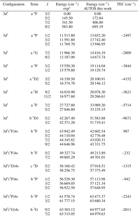
3d3 a4F 3/2 0.00 0.00 5/2 145.50 172.84 7/2 341.50 406.80 9/2 583.80 695.19 3d3 a4P 1/2 11 513.80 13 652.20 –2497 3/2 11 591.80 13 742.40 5/2 11 769.70 13 946.95 3d3 a2G 7/2 11 966.30 14 416.19 –2809 9/2 12 187.00 14 673.74 3d3 a2P 3/2 15 550.30 19 114.04 –3844 1/2 15 579.80 19 129.74 3d3 a2D2 3/2 16 330.50 20 100.91 –4152 5/2 16 374.70 20 146.12 3d3 a2H 9/2 16 810.90 20 078.30 –3621 11/2 16 977.60 20 266.61 3d3 a2F 7/2 27 727.80 33 089.20 –5714 5/2 27 846.80 33 235.15 3d3 b2D1 5/2 42 267.40 51 583.88 –9671 3/2 42 371.20 51 719.41 3d2(3F)4s b4F 3/2 43 942.49 42 602.54 987 5/2 44 110.04 42 776.48 7/2 44 345.82 43 020.31 9/2 44 646.96 43 331.75 3d2(3F)4s b2F 5/2 49 327.74 49 213.89 –232 7/2 49 805.29 49 701.01 3d2(1D)4s c2D 5/2 56 160.42 57 018.51 –1315 3/2 56 256.75 57 375.49 3d2(3P)4s b4P 1/2 56 529.30 57 113.98 –942 3/2 56 669.05 57 121.34 5/2 56 922.50 57 648.95 3d2(3P)4s b2P 1/2 61 578.74 63 473.37 –2243 3/2 61 777.15 63 680.34 3d2(1G)4s b2G 9/2 63 303.12 64 977.65 –2011 7/2 63 315.05 64 979.63
Table A.4. Level energies and TEC as used in the final AUTOSTRUCTURE calculation for Cr III.
Configuration Term J Energy (cm−1) Energy (cm−1) TEC (cm−1)
expa AUTOS this work
3d4 5D 0 0.00 0.00 1 61.76 72.10 2 182.44 212.23 3 356.00 413.38 4 575.73 667.53 3d4 3P2 0 16 770.26 21 192.58 –4915.57 1 17 167.54 21 662.36 2 17 850.13 22 471.78 3d4 3H 4 17 272.67 20 687.35 –3777.27 5 17 395.84 20 820.46 6 17 529.68 20 965.53 3d4 3F2 2 18 451.06 22 668.10 –4562.99 3 18 510.09 22 715.40 4 18 582.39 22 781.68 3d4 3G 3 20 702.45 24 870.64 –4539.61 4 20 851.87 25 036.46 5 20 995.16 25 180.98 3d4 1G2 4 25 137.91 30 614.62 –5849.22 3d4 3D 3 25 725.24 30 942.41 –5587.49 2 25 779.72 31 020.76 1 25 847.28 31 103.39 3d4 1I 6 26 014.10 31 029.76 –5375.59 3d4 1S2 0 27 371.30 33 703.73 –6697.38 3d4 1D2 2 32 150.53 39 577.20 –7791.24 3d4 1F 3 37 004.38 44 667.58 –8017.08 3d4 3F 1 4 43 285.81 52 959.22 –10 056.77 2 43 303.26 53 021.44 3 43 321.22 53 023.09 3d4 3P1 2 43 440.85 53 197.24 –10 169.68 1 43 915.56 53 778.08 0 44 140.06 54 054.51 3d3(4F)4s 5F 1 49 491.59 47 953.66 1164.64 2 49 627.27 48 093.91 3 49 828.04 48 301.53 4 50 090.28 48 573.13 5 50 409.28 48 903.99 3d4 1G1 4 49 767.47 60 658.94 –11 253.34 3d3(4F)4s 3F 2 56 650.51 56 473.01 –183.70 3 56 992.24 56 820.55 4 57 422.53 57 260.48 3d3(4P)4s 5P 1 63 044.61 63 794.02 –1103.74 2 63 173.17 63 925.05 3 63 420.87 64 170.86 3d4 1D1 2 65 762.08 79 930.56 –14 372.18
Table A.4. continued.
Configuration Term J Energy (cm−1) Energy (cm−1) TEC (cm−1)
expa AUTOS this work
3d3(2G)4s 3G 3 65 891.35 67 025.35 –1499.78 4 66 028.88 67 171.85 5 66 224.05 67 374.97 3d3(4P)4s 3P 0 69 600.40 71 852.36 –2565.55 1 69 780.80 72 045.17 2 70 291.77 72 414.33 3d3(2G)4s 1G 4 69 658.70 71 443.26 –2139.88 3d3(2P)4s 3P 2 70 189.89 72 689.00 –2714.90 1 70 344.55 72 680.44 0 70 485.87 72 797.09 3d3(2D2)4s 3D 1 70 980.15 73 670.82 –3080.44 3 71 321.98 74 026.92 2 71 322.09 73 991.69 3d3(2H)4s 3H 4 71 676.22 73 529.26 –2219.33 5 71 736.45 73 594.55 6 71 869.19 73 734.03 3d3(2P)4s 1P 1 73 880.42 77 033.83 –3537.93 3d3(2D2)4s 1D 2 74 787.89 78 006.10 –3721.63 3d3(2H)4s 1H 5 75 350.49 77 850.82 –2860.30 3d3(2F)4s 3F 4 84 372.87 88 718.77 –4706.52 3 84 483.43 88 830.70 2 84 571.41 88 919.37 3d3(2F)4s 1F 3 87 769.57 92 899.43 –5490.82
Table A.5. Level energies and TEC as used in the final AUTOSTRUCTURE calculation for Mn III.
Configuration Term J Energy (cm−1) Energy (cm−1) TEC (cm−1)
expa AUTOS this work
3d5 a6S 5/2 0.00 0.00 3d5 a4G 11/2 26 824.40 31 472.00 –4668 9/2 26 851.10 31 519.63 7/2 26 859.90 31 542.56 5/2 26 857.80 31 550.46 3d5 a4P 5/2 29 167.70 35 329.05 –6203 3/2 29 207.30 35 395.22 1/2 29 241.40 35 458.43 3d5 a4D 7/2 32 307.30 38 202.30 –5927 1/2 32 368.90 38 316.75 5/2 32 383.70 38 338.04 3/2 32 384.70 38 347.26 3d5 a2I 11/2 39 174.40 45 778.12 –6592 13/2 39 176.50 45 761.33 3d5 a2D3 5/2 41 238.10 49 473.09 3/2 41 569.80 49 849.49 3d5 a2F1 7/2 42 606.50 51 118.38 –8339
Table A.5. continued.
Configuration Term J Energy (cm−1) Energy (cm−1) TEC (cm−1)
expa AUTOS this work
5/2 43 105.40 51 705.69 3d5 a4F 9/2 43 573.16 52 018.22 –8479 7/2 43 602.50 52 095.26 5/2 43 668.84 52 219.81 3/2 43 674.70 52 226.94 3d5 a2H 9/2 46 515.90 55 354.79 –8973 11/2 46 670.70 55 574.70 3d5 a2G2 7/2 47 842.00 56 423.52 33 838 9/2 48 005.20 56 662.09 3d5 b2F2 5/2 51 002.70 60 322.59 –9396 7/2 51 059.70 60 413.02 3d5 a2S 1/2 55 677.70 66 087.97 10 419 3d5 b2D2 3/2 61 580.20 73 621.88 12 064 5/2 61 603.80 73 660.83 3d4(5D)4s a6D 1/2 62 456.99 61 319.67 1120 3/2 62 568.08 61 434.01 5/2 62 747.50 61 619.69 7/2 62 988.92 61 870.11 9/2 63 285.37 62 177.59 3d5 b2G1 7/2 68 892.00 81 837.14 89 9/2 68 899.20 81 802.79 3d4(5D)4s b4D 1/2 71 395.27 71 298.74 –4582 3/2 71 564.21 71 471.25 5/2 71 831.98 71 745.70 7/2 72 183.33 72 107.28 3d5 a2P 3/2 83 176.00 99 257.61 12 083 1/2 83 229.00 99 260.35 3d4(3P2)4s b4P 1/2 84 610.53 88 342.26 –3837 3/2 85 173.88 88 931.66 5/2 86 051.50 89 857.40 3d4(3H)4s a4H 7/2 84 981.63 87 328.94 –2346 9/2 85 077.09 87 427.16 11/2 85 200.76 87 550.50 13/2 85 346.72 87 695.80 3d4(3F2)4s b4F 3/2 86 486.77 89 842.48 –3347 5/2 86 520.94 89 868.81 7/2 86 578.24 89 915.78 9/2 86 654.07 89 985.57 3d4(3G)4s b4G 5/2 88 880.08 92 197.22 –3322 7/2 89 052.44 92 370.06 9/2 89 204.69 92 516.55 11/2 89 307.22 92 601.16 3d5 c2D1 5/2 89 496.30 10 7883.18 3/2 89 543.40 10 7937.61 3d4(3P2)4s b2P 1/2 90 233.50 94 577.75 –8322 3/2 91 308.30 95 704.86 3d4(3H)4s b2H 9/2 90 440.50 93 416.51 –2960
Table A.5. continued.
Configuration Term J Energy (cm−1) Energy (cm−1) TEC (cm−1)
expa AUTOS this work
11/2 90 746.06 93 716.86 3d4(3F2)4s c2F 5/2 91 906.10 95 885.05 –3970 7/2 91 948.30 95 904.47 3d4(3G)4s c2G 7/2 94 397.20 98 347.99 –3938 9/2 94 707.20 98 627.28 3d4(3D)4s c4D 7/2 94 697.85 99 265.73 5/2 94 771.47 99 351.54 3/2 94 850.66 99 438.56 1/2 94 906.45 99 496.18 3d4(1G2)4s d2G 9/2 96 430.40 10 1217.41 –4810 7/2 96 487.50 10 1254.17 3d4(1I)4s b2I 13/2 97 239.86 10 1268.32 –4029 11/2 97 271.76 10 1280.94 3d4(1S2)4s b2S 1/2 98 960.70 10 4949.13 3d4(3D)4s d2D 5/2 10 0001.30 10 5131.19 –5162 3/2 10 0085.20 10 5255.19 3d4(1D2)4s e2D 5/2 10 4470.80 11 1409.59 –6947 3/2 10 4517.90 11 1436.58 3d4(1F)4s d2F 7/2 10 9861.35 11 7115.27 –7280 5/2 10 9864.40 11 7119.66
Table A.6. Level energies and TEC as used in the final AUTOSTRUCTURE calculation for Fe III.
Configuration Term J Energy (cm−1) Energy (cm−1) TEC (cm−1)
expa AUTOS this work
3d6 5D 4 0.00 0.00 3 435.80 507.10 2 738.55 862.97 1 932.06 1091.89 0 1027.00 1204.04 3d6 3P2 2 19 404.19 23 647.18 –4737 1 20 687.78 25 059.72 0 21 207.76 25 649.67 3d6 3H 6 20 051.10 23 394.24 –3802 5 20 300.32 23 698.76 4 20 481.58 23 931.40 3d6 3F2 4 21 461.67 25 801.21 –4791 3 21 699.44 26 073.14 2 21 856.76 26 252.78 3d6 3G 5 24 558.25 29 192.43 –5133 4 24 940.95 29 644.65 3 25 142.00 29 894.20 3d5(6S)4s 7S 3 30 089.42 30 029.61 –366 3d6 1I 6 30 355.52 35 454.70 –5534 3d6 3D 2 30 715.68 37 203.58 –6915
Table A.6. continued.
Configuration Term J Energy (cm−1) Energy (cm−1) TEC (cm−1)
expa AUTOS this work
1 30 725.34 37 219.16 3 30 857.32 37 341.52 3d6 1G2 4 30 886.01 37 173.51 –6742 3d6 1S2 0 34 811.74 43 025.47 –8668 3d6 1D2 2 35 802.99 42 863.72 –7500 3d5(6S)4s 5S 2 41 000.09 42 950.74 –2376 3d6 1F 3 42 896.90 51 453.84 –8975 3d6 3P1 0 49 149.27 60 520.89 –11 839 1 49 576.82 60 964.56 2 50 411.69 61 828.63 3d6 3F1 2 50 184.65 61 680.59 –11 882 4 50 275.84 61 681.47 3 50 294.89 61 742.81 3d6 1G1 4 57 221.01 69 422.01 –12 637 3d5(4G)4s 5G 6 63 425.49 68 373.14 –5395 5 63 466.67 68 421.76 4 63 487.08 68 450.62 3 63 494.38 68 466.20 2 63 494.58 68 473.44 3d5(4P)4s 5P 3 66 464.80 73 367.40 –7365 2 66 523.02 73 432.03 1 66 591.78 73 514.33 3d5(4D)4s 5D 4 69 695.89 76 285.20 –7040 0 69 747.69 76 369.37 1 69 788.23 76 412.83 3 69 836.89 76 453.43 2 69 837.89 76 463.09 3d5(4G)4s 3G 5 70 694.17 76 977.86 –6742 3 70 725.22 77 054.02 4 70 728.93 77 034.71 3d5(4P)4s 3P 2 73 727.79 81 960.38 –8711 1 73 849.13 82 093.60 0 73 936.03 82 194.55 3d5(4D)4s 3D 3 76 956.76 84 898.92 –8401 1 77 075.39 85 060.78 2 77 102.41 85 079.33 3d6 1D 2 77 044.53 94 090.72 –17 060 3d5(2I)4s 3I 7 79 840.19 86 694.22 –7300 6 79 844.83 86 706.95 5 79 860.50 86 725.28
Table A.7. Level energies and TEC as used in the final AUTOSTRUCTURE calculation for Co III.
Configuration Term J Energy (cm−1) Energy (cm−1) TEC (cm−1)
expa AUTOS this work
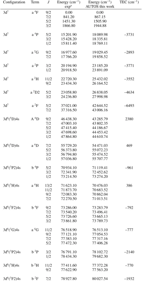
3d7 a4F 9/2 0.00 0.00 7/2 841.20 867.15 5/2 1451.30 1505.90 3/2 1866.80 1944.88 3d7 a4P 5/2 15 201.90 18 089.98 –3731 3/2 15 428.20 18 335.81 1/2 15 811.40 18 769.11 3d7 a2G 9/2 16 977.60 19 029.45 –2893 7/2 17 766.20 19 858.52 3d7 a2P 3/2 20 194.90 23 185.20 –3771 1/2 20 918.50 23 891.09 3d7 a2H 11/2 22 720.30 25 432.02 –3552 9/2 23 434.30 26 164.52 3d7 a2D2 5/2 23 058.80 26 838.05 –4634 3/2 24 236.80 27 998.98 3d7 a2F 5/2 37 021.00 42 644.52 –6493 7/2 37 316.50 43 006.16 3d6(5D)4s A6D 9/2 46 438.30 43 285.79 2380 7/2 47 003.10 43 802.35 5/2 47 415.40 44 186.67 3/2 47 698.60 44 453.42 1/2 47 864.80 44 610.74 3d6(5D)4s a4D 7/2 55 729.20 54 471.03 469 5/2 56 373.80 55 072.23 3/2 56 794.80 55 474.52 1/2 57 036.80 55 707.77 3d6(3P2)4s b4P 5/2 70 934.10 71 119.41 –961 3/2 72 341.90 72 452.62 1/2 73 214.50 73 274.20 3d6(3H)4s a4H 13/2 71 623.10 70 476.03 386 11/2 71 873.70 70 683.52 9/2 72 083.30 70 862.04 7/2 72 270.50 71 013.51 3d6(3F2)4s b4F 9/2 73 286.00 73 283.79 –792 7/2 73 540.20 73 496.41 5/2 73 726.60 73 665.13 3/2 73 861.80 73 789.73 3d6(3G)4s a4G 11/2 76 518.90 76 513.10 –777 9/2 77 121.10 77 054.53 7/2 77 383.10 77 317.16 5/2 77 472.30 77 406.28 3d6(3P2)4s b2P 3/2 76 791.10 78 102.72 –2140 1/2 78 434.30 79 682.30 3d6(3H)4s b2H 11/2 77 411.60 77 372.28 –770 9/2 77 622.90 77 563.20 3d6(3F2)4s b2F 7/2 78 927.80 80 027.54 –1932
Table A.7. continued.
Configuration Term J Energy (cm−1) Energy (cm−1) TEC (cm−1)
expa AUTOS this work
5/2 79 425.30 80 467.23 3d6(3G)4s b2G 9/2 82 363.30 83 470.73 –1933 7/2 82 920.70 83 997.43 3d6(3D)4s b4D 3/2 83 773.40 85 489.81 –2561 1/2 83 789.30 85 483.39 5/2 83 799.60 85 535.53 7/2 83 938.90 85 665.80 3d6(1I)4s a2I 13/2 85 474.10 85 538.64 –879 11/2 85 517.30 85 553.50 3d6(1G2)4s c2G 9/2 86 283.80 87 559.33 –2110 7/2 86 327.10 87 584.76
Table A.8. Level energies and TEC as used in the final AUTOSTRUCTURE calculation for Ni III.
Configuration Term J Energy (cm−1) Energy (cm−1) TEC (cm−1)
expa AUTOS this work
3d8 3F 4 0.00 0.00 3 1360.70 1472.24 2 2269.60 2468.98 3d8 1D 2 14 031.60 16 842.26 –3666 3d8 3P 2 16 661.60 20 528.23 –5035 1 16 977.80 21 006.68 0 17 230.70 21 293.86 3d8 1G 4 23 108.70 27 445.30 –5340 3d8 1S 0 52 532.00 65 278.00 –13 764 3d7(4F)4s 5F 5 53 703.93 53 005.75 –296 4 54 657.83 53 960.13 3 55 406.29 54 711.95 2 55 952.21 55 263.92 1 56 308.24 55 625.51 3d7(4F)4s 3F 4 61 338.58 61 734.69 –1404 3 62 605.58 63 016.75 2 63 471.93 63 906.28 3d7(4P)4s 5P 3 71 067.35 74 699.72 –4635 2 71 384.10 75 018.39 1 71 842.42 75 482.14 3d7(2G)4s 3G 5 75 123.65 77 321.56 –3178 4 75 646.61 77 843.80 3 76 237.25 78 411.25 3d7(4P)4s 3P 2 78 303.54 82 010.96 –4545 1 78 482.43 82 367.83 0 78 657.55 82 466.04 3d7(2P)4s 3P 2 79 143.01 83 532.03 –5487 1 79 749.22 83 850.82 0 80 621.10 84 804.55 3d7(2G)4s 1G 4 79 250.11 82 004.38 –3749
Table A.8. continued.
Configuration Term J Energy (cm−1) Energy (cm−1) TEC (cm−1)
expa AUTOS this work
3d7(2H)4s 3H 6 81 686.80 84 968.06 –4274 5 82 193.80 85 463.96 4 82 826.40 86 063.23 3d7(2D)4s 3D 3 82 172.60 86 627.94 –5479 1 82 277.26 88 786.80 2 83 033.45 87 434.51 3d7(2P)4s 1P 1 84 604.10 86 420.10 –4696 3d7(2H)4s 1H 5 85 834.20 89 665.91 –4850 3d7(2D)4s 1D 2 86 645.88 91 555.04 –5963 3d7(2F)4s 3F 2 97 841.60 10 5278.78 –8437 3 97 995.81 10 5430.55 4 98 237.93 10 5657.60 3d7(2F)4s 1F 3 10 1954.90 10 9886.32 –8942
Table A.9. Comparison of transition probabilities for M1 and E2 lines from our calculations (HFR and AUTOS) and previous works in Sc III. A[B] denotes A × 10B.
Lower level Upper level λ (nm) A(M1+E2) (s−1)
Type HFR AUTOS Others
3d2D 3/2 3d2D5/2 50 597.04 M1+E2 8.36[–05] 8.33[–05] 8.32[–05]a, 8.32[-05]b, 8.24[–05]c,8.33[–05]d 3d2D 3/2 4s2S1/2 391.55 M1+E2 7.67 8.71 8.21a, 7.95b, 7.86c, 7.83d 3d2D 5/2 4s2S1/2 394.61 E2 11.07 12.56 11.9a, 11.5b, 11.41c, 11.40d References.(a)Ali & Kim(1988);(b)Zeippen(1990);(c)Sahoo et al.(2008) and(d)Nandy et al.(2011).
Table A.10. Comparison of total (M1+E2) transition probabilities from our calculations (HFR and AUTOS) and previous works in Ti III. A[B] denotes A × 10B.
Lower level Upper level λ (nm) A(M1+E2) (s−1)
Config. Term J Config. Term J HFR AUTOS SSTa MCDFb
3d2 3F 3 3d4s 3D 3 261.49 1.24[+01] 1.26[+01] 1.10[+01] 1.26[+01] 3d2 3F 2 3d4s 3D 2 261.81 1.64[+01] 1.68[+01] 1.47[+01] 1.67[+01] 3d2 3F 2 3d4s 3D 1 262.74 3.75[+01] 3.83[+01] 3.40[+01] 3.82[+01] 3d2 3F 3 3d4s 3D 2 263.05 2.79[+01] 2.85[+01] 2.48[+01] 2.84[+01] 3d2 3F 4 3d4s 3D 3 263.10 4.28[+01] 4.37[+01] 3.78[+01] 4.35[+01] 3d2 3F 3 3d4s 3D 1 263.99 1.83[+01] 1.87[+01] 1.65[+01] 1.86[+01] 3d2 3F 4 3d4s 3D 2 264.68 1.16[+01] 1.19[+01] 1.04[+01] 1.18[+01] 3d2 1D 2 3d4s 1D 2 300.93 2.07[+01] 2.09[+01] 1.94[+01] 1.89[+01] 3d2 1G 4 3d4s 1D 2 366.21 1.62[+01] 1.64[+01] 1.47[+01] 1.48[+01] 3d2 1D 2 3d2 1S 0 416.63 6.51[+00] 6.43[+00] 7.13[+00] 4.95[+00] 3d2 3F 3 3d2 1G 4 703.55 4.11[–03] 6.61[–03] 6.84[–03] 4.50[–03] 3d2 3F 4 3d2 1G 4 715.33 6.53[–03] 1.05[–02] 1.07[–02] 7.14[–03] 3d2 3F 2 3d2 3P 1 943.84 1.34[–02] 1.32[–02] 1.38[–02] 1.39[–02] 3d2 3F 3 3d2 3P 2 948.29 7.89[–03] 7.80[–03] 8.14[–03] 8.13[–03] 3d2 3F 2 3d2 3P 0 949.45 3.91[–02] 3.85[–02] 3.99[–02] 4.05[–02] 3d2 3F 3 3d2 3P 1 960.17 2.46[–02] 2.42[–02] 2.48[–02] 2.55[–02] 3d2 3F 4 3d2 3P 2 969.81 2.69[–02] 2.62[–02] 2.66[–02] 2.77[–02] 3d2 3F 2 3d2 1D 2 1180.65 5.05[–03] 7.92[–03] 8.27[–03] 5.47[–03] 3d2 3F 3 3d2 1D 2 1206.31 9.43[–03] 1.47[–02] 1.51[–02] 1.02[–02] 3d2 3F 3 3d2 3F 4 42 730.85 2.60[–04] 2.64[–04] 4.80[–04] 2.65[–04] 3d2 3F 2 3d2 3F 3 55 508.75 1.51[–04] 1.62[–04] 2.99[–04] 1.63[–04]
Table A.11. Comparison of total (M1+E2) transition probabilities from our calculations (HFR and AUTOS) and previous works in V III. A[B] denotes A × 10B.
λ (nm) Lower level Upper level A(M1+E2) (s−1)
E(cm−1) Config. Term J E (cm−1) Config. Term J HFR AUTOS
176.74 341.50 3d3 4F 7/ 2 56 922.50 3d24s 4P 5/2 2.60[+01] 2.61[+01] 176.90 0.00 3d3 4F 3/ 2 56 529.30 3d24s 4P 1/2 8.77[+01] 8.98[+01] 176.92 145.50 3d3 4F 5/ 2 56 669.05 3d24s 4P 3/2 4.68[+01] 4.85[+01] 177.36 145.50 3d3 4F 5/ 2 56 529.30 3d24s 4P 1/2 5.78[+01] 5.91[+01] 177.50 583.80 3d3 4F 9/ 2 56 922.50 3d24s 4P 5/2 8.03[+01] 8.02[+01] 177.53 341.50 3d3 4F 7/ 2 56 669.05 3d24s 4P 3/2 6.53[+01] 6.75[+01] 179.93 583.80 3d3 4F 9/ 2 56 160.42 3d24s 2D 5/2 2.09[+01] 2.32[+01] 194.75 11 966.30 3d3 2G 7/ 2 63 315.05 3d24s 2G 7/2 4.69[+01] 4.89[+01] 195.63 12 187.00 3d3 2G 9/ 2 63 303.12 3d24s 2G 9/2 4.98[+01] 5.25[+01] 215.03 16 810.90 3d3 2H 9/ 2 63 315.05 3d24s 2G 7/2 7.66[+01] 7.86[+01] 215.86 16 977.60 3d3 2H 11/ 2 63 303.12 3d24s 2G 9/2 7.24[+01] 7.39[+01] 216.46 15 579.80 3d3 2P 1/ 2 61 777.15 3d24s 2P 3/2 1.30[+01] 1.40[+01] 217.26 15 550.30 3d3 2P 3/ 2 61 578.74 3d24s 2P 1/2 4.23[+01] 4.79[+01] 220.04 16 330.50 3d3 2D 3/ 2 61 777.15 3d24s 2P 3/2 2.14[+01] 2.40[+01] 220.25 16 374.70 3d3 2D 5/ 2 61 777.15 3d24s 2P 3/2 1.44[+01] 1.77[+01] 220.60 11 591.80 3d3 4P 3/ 2 56 922.50 3d24s 4P 5/2 1.81[+01] 1.77[+01] 221.22 16 374.70 3d3 2D 5/ 2 61 578.74 3d24s 2P 1/2 8.05[+00] 9.91[+00] 222.72 11 769.70 3d3 4P 5/ 2 56 669.05 3d24s 4P 3/2 3.12[+01] 3.23[+01] 223.42 11 769.70 3d3 4P 5/ 2 56 529.30 3d24s 4P 1/2 4.99[+01] 5.12[+01] 225.71 341.50 3d3 4F 7/ 2 44 646.96 3d24s 4F 9/2 1.74[+01] 1.79[+01] 225.78 11 966.30 3d3 2G 7/ 2 56 256.75 3d24s 2D 3/2 3.88[+01] 4.01[+01] 226.24 145.50 3d3 4F 5/ 2 44 345.82 3d24s 4F 7/2 2.38[+01] 2.45[+01] 226.71 0.00 3d3 4F 3/ 2 44 110.04 3d24s 4F 5/2 2.41[+01] 2.48[+01] 226.95 583.80 3d3 4F 9/ 2 44 646.96 3d24s 4F 9/2 5.94[+01] 6.11[+01] 227.25 341.50 3d3 4F 7/ 2 44 345.82 3d24s 4F 7/2 3.06[+01] 3.15[+01] 227.41 12 187.00 3d3 2G 9/ 2 56 160.42 3d24s 2D 5/2 2.95[+01] 2.93[+01] 227.46 145.50 3d3 4F 5/ 2 44 110.04 3d24s 4F 5/2 1.99[+01] 2.05[+01] 227.57 0.00 3d3 4F 3/ 2 43 942.49 3d24s 4F 3/2 3.68[+01] 3.79[+01] 228.33 145.50 3d3 4F 5/ 2 43 942.49 3d24s 4F 3/2 3.49[+01] 3.59[+01] 228.47 341.50 3d3 4F 7/ 2 44 110.04 3d24s 4F 5/2 3.02[+01] 3.11[+01] 228.51 583.80 3d3 4F 9/ 2 44 345.82 3d24s 4F 7/2 2.05[+01] 2.11[+01] 246.24 15 550.30 3d3 2P 3/ 2 56 160.42 3d24s 2D 5/2 1.43[+01] 1.45[+01] 250.46 16 330.50 3d3 2D 3/ 2 56 256.75 3d24s 2D 3/2 2.17[+01] 2.26[+01] 251.35 16 374.70 3d3 2D 5/ 2 56 160.42 3d24s 2D 5/2 1.57[+01] 1.59[+01] 265.83 12 187.00 3d3 2G 9/ 2 49 805.29 3d24s 2F 7/2 2.71[+01] 2.87[+01] 267.66 11 966.30 3d3 2G 7/ 2 49 327.74 3d24s 2F 5/2 2.72[+01] 2.91[+01] 293.69 27 727.80 3d3 2F 7/ 2 61 777.15 3d24s 2P 3/2 2.35[+01] 2.46[+01] 296.45 27 846.80 3d3 2F 5/ 2 61 578.74 3d24s 2P 1/2 2.73[+01] 2.88[+01] 299.13 16 374.70 3d3 2D 5/ 2 49 805.29 3d24s 2F 7/2 6.46[+00] 6.68[+00] 304.62 16 977.60 3d3 2H 11/ 2 49 805.29 3d24s 2F 7/2 2.09[+01] 2.22[+01] 307.53 16 810.90 3d3 2H 9/ 2 49 327.74 3d24s 2F 5/2 2.01[+01] 2.12[+01] 328.89 11 966.30 3d3 2G 7/ 2 42 371.20 3d3 2D 3/2 4.99[+00] 5.31[+00] 332.44 12 187.00 3d3 2G 9/ 2 42 267.40 3d3 2D 5/2 4.46[+00] 4.75[+00] 372.84 15 550.30 3d3 2P 3/ 2 42 371.20 3d3 2D 3/2 8.66[–01] 1.07[+00] 612.35 0.00 3d3 4F 3/ 2 16 330.50 3d3 2D 3/2 2.12[–02] 3.04[–02] 617.86 145.50 3d3 4F 5/ 2 16 330.50 3d3 2D 3/2 3.83[–02] 5.65[–02] 623.71 341.50 3d3 4F 7/ 2 16 374.70 3d3 2D 5/2 5.62[–02] 7.47[–02] 629.70 11 966.30 3d3 2G 7/ 2 27 846.80 3d3 2F 5/2 9.55[–02] 9.91[–02] 634.46 11 966.30 3d3 2G 7/ 2 27 727.80 3d3 2F 7/2 2.05[–02] 2.58[–02] 643.07 0.00 3d3 4F 3/ 2 15 550.30 3d3 2P 3/2 1.50[–02] 1.97[–02] 643.47 12 187.00 3d3 2G 9/ 2 27 727.80 3d3 2F 7/2 8.62[–02] 8.97[–02] 649.15 145.50 3d3 4F 5/ 2 15 550.30 3d3 2P 3/2 2.53[–02] 3.32[–02] 844.20 341.50 3d3 4F 7/ 2 12 187.00 3d3 2G 9/2 1.20[–02] 1.67[–02] 845.97 145.50 3d3 4F 5/ 2 11 966.30 3d3 2G 7/2 1.10[–02] 1.59[–02] 860.23 341.50 3d3 4F 7/ 2 11 966.30 3d3 2G 7/2 1.24[–02] 1.80[–02] 861.83 583.80 3d3 4F 9/ 2 12 187.00 3d3 2G 9/2 3.12[–02] 4.39[–02] 862.68 0.00 3d3 4F 3/ 2 11 591.80 3d3 4P 3/2 5.79[–03] 5.78[–03] 868.52 0.00 3d3 4F 3/ 2 11 513.80 3d3 4P 1/2 2.79[–02] 2.75[–02] 873.64 145.50 3d3 4F 5/ 2 11 591.80 3d3 4P 3/2 1.65[–02] 1.63[–02] 875.03 341.50 3d3 4F 7/ 2 11 769.70 3d3 4P 5/2 1.03[–02] 1.02[–02]
Table A.11. continued.
λ (nm) Lower level Upper level A(M1+E2) (s−1)
E(cm−1) Config. Term J E (cm−1) Config. Term J HFR AUTOS
879.64 145.50 3d3 4F 5/ 2 11 513.80 3d3 4P 1/2 1.74[–02] 1.71[–02] 880.82 16 374.70 3d3 2D 5/ 2 27 727.80 3d3 2F 7/2 1.85[–02] 2.03[–02] 888.87 341.50 3d3 4F 7/ 2 11 591.80 3d3 4P 3/2 2.12[–02] 2.08[–02] 893.98 583.80 3d3 4F 9/ 2 11 769.70 3d3 4P 5/2 2.88[–02] 2.84[–02] 906.13 16 810.90 3d3 2H 9/ 2 27 846.80 3d3 2F 5/2 2.81[–02] 2.82[–02] 930.22 16 977.60 3d3 2H 11/ 2 27 727.80 3d3 2F 7/2 2.32[–02] 2.33[–02] 2064.15 11 966.30 3d3 2G 7/ 2 16 810.90 3d3 2H 9/2 5.46[–03] 7.86[–03] 2087.42 12 187.00 3d3 2G 9/ 2 16 977.60 3d3 2H 11/2 5.39[–03] 7.76[–03] 2162.68 12 187.00 3d3 2G 9/ 2 16 810.90 3d3 2H 9/2 1.06[–02] 1.53[–02] 2192.60 11 769.70 3d3 4P 5/ 2 16 330.50 3d3 2D 3/2 7.36[–03] 8.90[–03] 2459.42 11 513.80 3d3 4P 1/ 2 15 579.80 3d3 2P 1/2 1.56[–02] 2.29[–02] 2526.21 11 591.80 3d3 4P 3/ 2 15 550.30 3d3 2P 3/2 8.75[–03] 1.32[–02] 41 271.15 341.50 3d3 4F 7/ 2 583.80 3d3 4F 9/2 3.85[–04] 3.84[–04] 51 124.74 145.50 3d3 4F 5/ 2 341.10 3d3 4F 7/2 3.26[–04] 3.24[–04] 68 728.52 0.00 3d3 4F 3/ 2 145.50 3d3 4F 5/2 1.33[–04] 1.33[–04]
Table A.12. Theoretical lifetimes obtained in this work for VIII using the HFR and AUTOS methods compared to the previous MCHF results of
Irimia(2007). A[B] denotes A × 10B.
Config. Term J Lifetime (ns)
HFR AUTOS Previousa 3d3 a4F 5/2 7.49[+03] 7.53[+03] 4.20[+03] 7/2 3.07[+03] 3.08[+03] 2.06[+03] 9/2 2.60[+03] 2.61[+03] 2.47[+03] 3d3 a4P 1/2 2.21[+01] 2.24[+01] 2.30[+01] 3/2 2.30[+01] 2.33[+01] 2.37[+01] 5/2 2.38[+01] 2.41[+01] 2.52[+01] 3d3 a2G 7/2 4.13[+01] 2.86[+01] 7.65[+02] 9/2 2.30[+01] 1.65[+01] 4.94[+03] 3d3 a2P 3/2 1.71[+01] 1.23[+01] 9.82[+02] 1/2 6.19[+01] 4.22[+01] 1.19[+04] 3d3 a2D2 3/2 1.37[+01] 9.85[+00] 4.48[+04] 5/2 1.40[+01] 1.07[+01] 3.27[+03] 3d3 a2H 9/2 6.17[+01] 4.28[+01] 1.43[+04] 11/2 1.82[+02] 1.27[+02] 6.00[+03] 3d3 a2F 7/2 5.67[+00] 5.06[+00] 8.21[+00] 5/2 5.83[+00] 5.40[+00] 7.28[+00] 3d3 b2D1 5/2 1.51[–01] 1.36[–01] 1.70[–01] 3/2 1.46[–01] 1.32[–01] 1.62[–01] 3d2(3F)4s b4F 3/2 1.24[–02] 1.21[–02] 1.16[–02] 5/2 1.23[–02] 1.20[–02] 1.14[–02] 7/2 1.22[–02] 1.18[–02] 1.13[–02] 9/2 1.20[–02] 1.17[–02] 1.12[–02] 3d2(3F)4s b2F 5/2 1.60[–02] 1.50[–02] 1.76[–02] 7/2 1.58[–02] 1.49[–02] 1.69[–02] 3d2(1D)4s c2D 5/2 8.91[–03] 8.52[–03] 1.11[–02] 3/2 9.73[–03] 9.55[–03] 1.12[–02] 3d2(3P)4s b4P 1/2 4.97[–03] 4.85[–03] 4.50[–03] 3/2 5.29[–03] 5.14[–03] 4.49[–03] 5/2 5.57[–03] 5.50[–03] 4.50[–03] 3d2(3P)4s b2P 1/2 1.26[–02] 1.13[–02] 1.30[–02] 3/2 1.26[–02] 1.13[–02] 1.25[–02] 3d2(1G)4s b2G 9/2 7.05[–03] 6.78[–03] 7.26[–03] 7/2 7.06[–03] 6.82[–03] 7.16[–03]