UNIVERSITÉ DE MONTRÉAL
REFINEMENT OF NON-SYNCHRONOUS VIBRATIONS PREDICTION IN
AXIAL COMPRESSORS
MARTIN DROLET
DÉPARTEMENT DE GÉNIE MÉCANIQUE ÉCOLE POLYTECHNIQUE DE MONTRÉAL
MÉMOIRE PRÉSENTÉ EN VUE DE L’OBTENTION DU DIPLÔME DE MAÎTRISE ÈS SCIENCES APPLIQUÉES
(GÉNIE MÉCANIQUE) DÉCEMBRE 2010
UNIVERSITÉ DE MONTRÉAL
ÉCOLE POLYTECHNIQUE DE MONTRÉAL
Ce mémoire intitulé:
REFINEMENT OF NON-SYNCHRONOUS VIBRATIONS PREDICTION IN AXIAL COMPRESSORS
Présenté par : DROLET Martin
en vue de l’obtention du diplôme de : Maîtrise ès sciences appliquées a été dûment accepté par le jury d’examen constitué de :
M.TRÉPANIER Jean-Yves, Ph.D., président
M.VO Huu Duc, Ph.D., membre et directeur de recherche
M.MUREITHI Njuki W., Ph.D., membre et codirecteur de recherche M.VÉTEL Jérome, Ph.D., membre
DÉDICACE
À Mélanie, Julie, Louise et Michel, pour votre amour, support et soutien durant toutes
iv
ACKNOWLEDGMENT
I would like to thank Pratt & Whitney Canada (P&WC), the Natural Science and Engineering Research Council of Canada (NSERC) and the Fond Québécois de Recherche sur la Nature et les Technologies (FQRNT) for funding and supporting this research initiative through an Industrial Innovative Scholarship (IIS). I would also like to thank P&WC for the authorization to publish this work. I am very grateful to Dr. Jean Thomassin for believing in me and for all the mentoring and numerous insightful discussions on non-synchronous vibrations.
Part of this project would not have been possible without the precious collaboration of the Special Tests organization at P&WC under the direction of Mr. Richard Lahaie who I am entirely grateful for his support. More specifically, I would like to thank the following people, in no particular order, for their contributions to the project: Patrick Rousseau, Benoît Patry, Daniel Summers-Lépine, Martin Cloutier, Renaud Lévesque, Yvon Michaud, Keith Ward, Michael W. Krieger, Jasmin Lamoureux, Michel Collin, André LeBlanc, Sylvain Bélanger and Sylvain Poupart. I would also like to acknowledge the support and mentoring of my director, Dr. Huu-Duc Vo and co-director, Dr. Njuki W. Mureithi. I would like to thank Benedict Besner and Kenny Huynh, from the lab at École Polytechnique de Montréal, for their help with the project. I am also very grateful to Shinya Ueno for his indescribable help with particle image velocimetry during the experimental tests.
Last, but not least, I would like to thank my girlfriend, Mélanie Brillant, my family: Julie Beaulieu-Drolet, Louise Beaulieu and Michel Drolet and my friends: Mathieu Côté, Martin Joly, Charles Paré, Laurence Côté, Mélissa Théorêt, Alexandre Charest and Alexandre Bernard, for all their motivation and support throughout my university studies. Without these precious people, I would certainly not be the person I am today and I am very grateful to them for what they all bring to my life.
RÉSUMÉ
Les vibrations asynchrones, ou NSV (de l’anglais « Non-Synchronous Vibrations »), ainsi que le flottement classique font parties de la famille des vibrations induites par les écoulements (ou FIV de l’anglais « Flow-Induced Vibrations ») observées dans les turbomachines. Les FIV sont habituellement causées par l’interaction des fluctuations de la charge aérodynamique sur une structure et la structure elle-même. Elles sont généralement classifiées en deux catégories distinctes, soient les réponses forcées et les instabilités fluide-élastiques qui regroupent, entre autres, les NSV et le flottement classique. Plusieurs cas de NSV ont été rapportés dans l’industrie, dans les étages avant de compresseurs axiaux, et sont typiquement reliées aux dommages en fatigue des aubes. Cependant, le mécanisme physique pouvant expliquer les NSV n’est pas entièrement compris et universellement accepté. Des études antérieures ont suggérées que les fluctuations de l’écoulement de jeu, qui surviennent plus souvent à haute charge aérodynamique et pour des jeux assez grands, pourraient expliquer les NSV. Une autre hypothèse suggère que les NSV découlent de l’impact de l’écoulement de jeu sur l’intrados d’une aube adjacente et que l’étude de la dynamique d’un jet impactant pourrait possiblement expliquer les NSV. Un modèle, basé sur l’analogie d’un jet impactant en résonance, a été proposé afin de prédire les vitesses critiques auxquelles les NSV peuvent survenir. Ce modèle a été statistiquement vérifié et validé expérimentalement. En dépit du fait que le modèle soit capable de fournir une bonne approximation a priori des vitesses critiques de NSV, il a été démontré expérimentalement que l’exactitude des prédictions découlant du modèle est très sensible à un paramètre k, qui a été définit comme étant le « coefficient de convection de l’instabilité ». En effet, les prédictions du modèle ne s’avèrent justes que si le coefficient k est connu.
Cet ouvrage présente une étude du modèle de NSV proposé, basé sur l’analogie du jet impactant en résonance décris précédemment, qui utilise principalement des outils numériques afin d’améliorer les prédictions des vitesses critiques de NSV. L’étude démontre que le paramètre « k » est influencé par la grandeur du jeu ainsi que la température d’opération. Cependant, l’effet dominant semble provenir de la grandeur du jeu alors que l’effet de la température sur « k » peut être négligé à des fins de conception. Les travaux suggèrent également que les résultats obtenus devraient être générique, i.e. indépendant de la géométrie utilisée. La principale contribution des travaux est donc une corrélation basée sur des résultats numériques, qui peut déterminer le
vi
paramètre k indépendamment de la géométrie, ce qui améliore de façon significative les prédictions de NSV d’après le modèle proposé et en fait un outil de conception pouvant être utilisé dès les premières étapes de conception d’un rotor de compresseur axial. De plus, cet ouvrage propose une configuration possible pour rencontrer les NSV en conditions d’étranglement alors qu’elles sont connues jusqu’à présent pour survenir près du décrochage.
ABSTRACT
Non-Synchronous Vibrations (NSV), along with classical flutter, are part of the Flow-Induced Vibrations (FIV) family observed in turbomachineries. FIV are typically caused by the interaction of the unsteady aerodynamic loading on a structure and the structure itself and can be generally classified into two categories, which are Forced Responses and Fluid-Elastic Instabilities. The latter regroups NSV and classical flutter. A number of NSV cases have been reported in the industry, in the front stages of axial compressors, and are typically known to cause high-cycle fatigue damages. However, the physical mechanism underlying NSV is not yet fully understood and universally accepted. Previous studies have suggested that the tip clearance flow oscillations, which are more likely to occur at large tip clearances and high aerodynamic blade loading, could explain NSV. It was also suggested that NSV could arise from the impingement of the tip clearance flow leakage on the blade pressure side and that the study of the dynamics of impinging jets could explain NSV. A model to predict the critical speed at which NSV are likely to occur was derived, based on the resonant impinging jet analogy. The model was statistically verified and experimentally demonstrated. Although the proposed model provides a very good approximation of the critical NSV speed, it was found very sensitive to what was defined as the “instability convection coefficient” (k). It was found from experiments that the proposed NSV model can only yield accurate predictions of the critical NSV speed if the k parameter is known. This work investigates NSV based on the proposed model and the resonant impinging jet analogy, mainly using CFD, to improve the critical NSV speed predictions. The results showed that the k parameter is influenced by both the tip clearance size and operating temperature. However, the dominant effect appears to come from the tip clearance size while the effect of temperature on k can be neglected for design purposes. In addition, this work suggests that the results should be generic, i.e. independent from the geometry used. The main contribution from the current Thesis is a correlation for the k parameter that is independent from the geometry, based on a numerical experiment, which significantly improves the critical NSV speed predictions and makes the proposed model independent from further experiments or numerical studies. In addition, this work also proposes a possible configuration to encounter NSV, which are typically known to occur near stall, in choked flow conditions.
viii
CONDENSÉ EN FRANÇAIS
Chapitre 1: Introduction.
De nos jours, les compagnies de turbines à gaz repoussent continuellement les limites en termes de ratio poussée/poids et de consommation spécifique des moteurs afin de demeurer compétitif sur le marché. La réduction constante du poids des pièces pose de nouveaux défis en ce qui a trait aux vibrations des diverses composantes. La compréhension des divers phénomènes de vibrations, souvent associés aux dommages en fatigue des pièces, est donc primordiale afin de profiter pleinement des avantages compétitifs sur le marché. Le présent ouvrage se concentre sur un type particulier de vibrations rencontrées dans les modules de compresseurs axiaux: les vibrations asynchrones, ou NSV (de l’anglais « Non-Synchronous Vibrations »).
Problématique et objectifs.
Un modèle, sous la forme d’une équation, a été développé par Thomassin, J., Vo, H.D. et Mureithi, N.W. (2008, 2009) et s’avère être un outil à la fois simple et puissant qui permet de déterminer les vitesses critiques de NSV. Cependant, les prédictions du modèle ne s’avèrent juste que lorsque la valeur exacte d’un paramètre k, défini comme le « coefficient de transport de l’instabilité en bout d’aube » est connue. En effet, l’approximation générale k=2 (Thomassin et
al., 2009) s’avère inadéquate pour déterminer de façon précise les vitesses critiques. L’objectif
principal du présent ouvrage consiste donc à utiliser la mécanique des fluides numériques afin d’améliorer les prédictions des vitesses critiques de NSV basées sur le modèle proposé par Thomassin et al. (2008, 2009). Plus spécifiquement, les objectifs sont :
• Estimer le paramètre « k » à l’aide d’un modèle numérique de l’écoulement et déterminer l’influence de la dimension du jeu et de la température d’opération sur sa valeur.
• Proposer une corrélation basée sur les résultats numériques permettant d’identifier le paramètre « k » pour une géométrie donnée afin d’améliorer les prédictions des vitesses critiques de NSV d’après le modèle de Thomassin et al. (2008, 2009).
• Examiner l’aspect générique, ou universel, des travaux par l’étude de la mécanique des fluides inhérente aux compresseurs axiaux et identifier la possibilité d’obtenir les NSV en condition d’étranglement du compresseur, par opposition aux conditions de décrochage où les NSV sont typiquement observées.
Chapitre 2 : Revue de la Littérature.
Historique des vibrations asynchrones.
Les compresseurs axiaux sont souvent assujettis aux vibrations qui sont généralement divisées en deux grandes catégories : les vibrations mécaniques, résultant de l’interaction physique entre les composantes, ainsi que les vibrations induites par l’écoulement, qui découlent souvent d’une interaction fluide-structure entre les aubes et l’écoulement de l’air. Cette dernière catégorie peut également être subdivisée en deux types distincts, soient les réponses forcées et les instabilités fluide-élastiques.
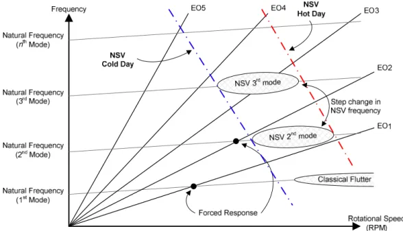
Les réponses forcées sont les vibrations les plus couramment rencontrées dans les compresseurs axiaux. Elles sont connues pour être « synchrones » avec la vitesse de rotation de l’arbre, ce qui signifie que la fréquence d’excitation sera un multiple entier de la fréquence de rotation de l’arbre, plus couramment désignée EO (de l’anglais « Engine Order »). Les vibrations asynchrones (NSV) quant à elles, ne surviennent pas nécessairement à un multiple entier de la fréquence de rotation de l’arbre.
Un cas typique d’instabilité fluide-élastique est connu sous le nom de « flottement ». Plusieurs types de flottement ont été répertoriés dans l’industrie (Dowell, E.H., Crawley, E.F., Curtiss Jr, .H.C., Peters, D.A., Scanlan, R.H. et Sisto, F., 1995) et ont été souvent confondus avec les vibrations asynchrones (NSV). Ceci explique pourquoi les cas de NSV n’ont été que vaguement répertoriés dans les 15 à 20 dernières années.
Un des premiers cas de NSV répertorié est attribué à Baumgartner M., Kamaler F. et Hourmouziadis J. (1995) qui ont fait le lien entre les instabilités rotatives (RI, de l’anglais « rotating instabilities ») à partir d’observations expérimentales. Les RI ont été grandement étudiées dans le passé comme une source d’excitation possible des aubes de compresseurs (Liu, J.M., Holste, F. et Neise, W., 1996; Kameier, F. et Neise, W., 1997a; Kameier, F. et Neise, W., 1997b; Mailach, R., Lehmann, I. et Vogeler, K., 2001a; Mailach, R., Sauer, H. et Vogeler, K., 2001b; März, J., Hah, C. et Neise, W., 2002). Elles ont été modélisées comme étant une source de bruit émanant des fluctuations de l’écoulement au bord d’attaque en bout d’aube, possiblement liées aux NSV.
Ce n’est qu’en 2003 que les instabilités rotatives ont reçu l’appellation « vibrations asynchrones » (NSV) par Kielb, R.E., Thomas, J.P., Barter, J.W. et Hall, K.C. (2003) qui ont démontrés l’effet
x
des conditions d’opérations, tel que la température, sur les NSV et ont fait le liens avec les instabilités de l’écoulement de jeu à l’aide de modèles numériques. Ils ont également observé un changement soudain des formes de mode en fréquence, pour des conditions d’opérations constantes, ce qui s’avère un phénomène caractéristique aux NSV. Par la suite, Vo, H.D. (2006) a observé que le refoulement de l’écoulement de jeu en bord de fuite pouvait possiblement agir comme un jet impactant sur l’aube adjacente, lorsque la charge aérodynamique est élevée. Ce phénomène a également été observé expérimentalement par Deppe, A., Saathoff, H. et Stark, U. (2005). Basé sur ses observations, Vo, H.D. (2006) a donc proposé d’étudier la dynamique d’un jet impactant comme une explication possible des vibrations asynchrones.
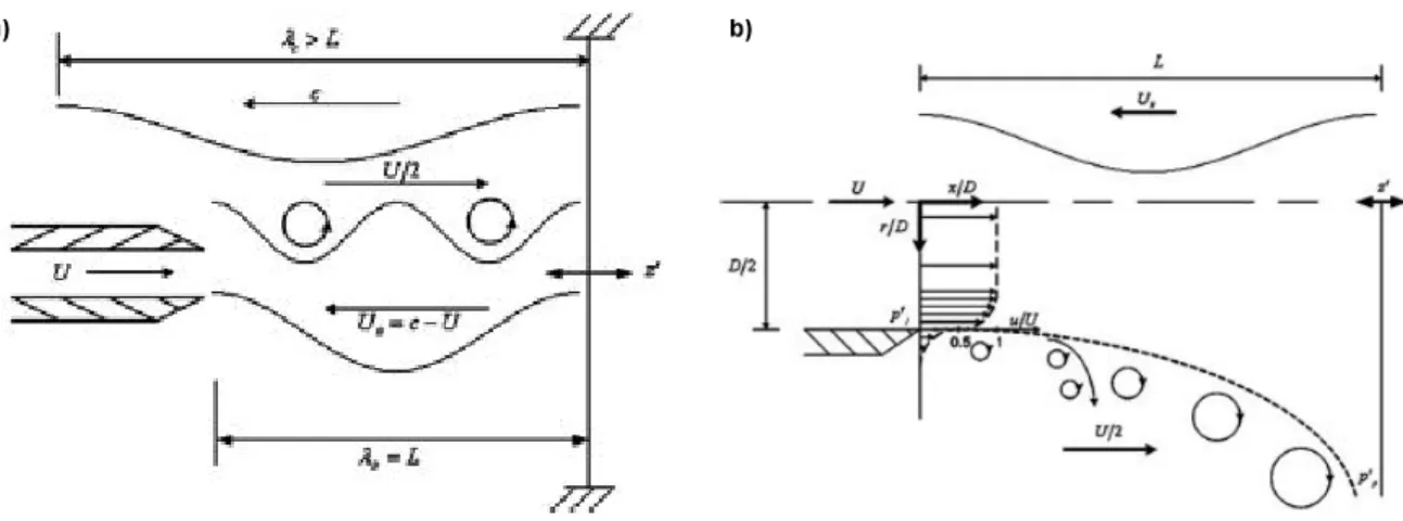
Théorie de la rétroaction d’onde dans le noyau potentiel d’un jet.
Thomassin et al. (2009) ont donc répété l’expérience d’un jet impactant sur une plaque de Ho, C.-M. et Nosseir, S. (1981). Par contre, leur plaque était flexible et en vibration afin de simuler une aube de compresseur en porte-à-faux. Cette plaque flexible permettait donc des fluctuations de pression au centre du jet, au point de stagnation, ce qui crée une onde de rétroaction additionnelle à l’intérieur même du noyau potentiel du jet. Par conséquent, cette nouvelle onde de rétroaction se propage à une vitesse UB de sorte que UB = c -U, où c est la vitesse du son locale (équation
(2.1), p.14). Afin que le jet entre en résonance, ceci implique que la fréquence réduite du jet doit satisfaire la condition définie à l’équation (2.2), p.14. Ils ont également trouvé que la distance jet-plaque (L) doit satisfaire L = nλB/2, où λB est la longueur de l’onde de rétroaction et n est un
multiple entier qui tient compte des super-harmoniques de la longueur d’onde (voir équation (2.3), p.14). Ces relations présentent donc la base derrière la théorie de la rétroaction d’onde dans le noyau potentiel d’un jet impactant (en anglais : « Jet-Core Feedback Theory ») proposée et validée expérimentalement par Thomassin et al. (2009).
Modèle de prédiction des vibrations asynchrones.
Thomassin et al. (2008, 2009) ont alors suggéré que lorsque certaines conditions d’opérations sont rencontrées (haute charge aérodynamique et vitesse du son adéquate), la résonance de l’écoulement de jeu, de façon analogue au modèle de l’onde de rétroaction dans le noyau potentiel d’un jet impactant, pouvait être le mécanisme physique derrière les NSV. Un modèle, sous la forme d’une équation (équation (2.4), p.17), a alors été proposé par Thomassin et al. (2009) afin de prédire la vitesse critique en bout d’aube à laquelle les NSV peuvent être
rencontrées. Dans cette équation, Utipc est la vitesse critique en bout d’aube à laquelle les NSV
devraient survenir, c est la vitesse du son en bout d’aube, s est le pas en bout d’aube (distance d’aube-en-aube), fb est la fréquence naturelle de l’aube et n est un multiple entier relié aux
super-harmoniques de l’onde de rétroaction acoustique. En utilisant l’égalité Utipc = k UF , où k est
définit comme étant le « coefficient de transport de l’instabilité en bout d’aube » (de l’anglais, « tip instability convection coefficient », Thomassin et al., 2009), on obtient une forme plus générale du modèle, tel que définit par l’équation (2.5) (p.17). Le modèle de NSV proposé par Thomassin et al. (2008, 2009) a été validé expérimentalement et il a été démontré que le paramètre « k » dans l’équation (2.5) discutée précédemment devait être connue afin que les prédictions des vitesses critiques de NSV s’avèrent justes. En effet, ils ont mesuré expérimentalement le paramètre « k » et les prédictions des vitesses critiques de NSV découlant de l’utilisation de la valeur adéquate de k étaient toutes à l’intérieur de 2% d’erreur par rapport aux vitesses critiques observées expérimentalement. L’approximation générale k=2 a démontrée des erreurs allant jusqu’à 20% pour les mêmes prédictions.
Modélisation numérique de la résonance de l’écoulement de jeu.
Une méthode numérique permettant d’améliorer les prédictions des vitesses critiques de NSV d’après le modèle de Thomassin et al. (2008, 2009) a également été développée par Drolet, M., Thomassin, J., Vo, H.D. et Mureithi, N.W. (2009). En effet, en utilisant une géométrie de compresseur identique à celle utilisée expérimentalement par Thomassin et al. (2008), ils ont démontré qu’un modèle de mécanique des fluides numérique, utilisant un maillage déformable afin de simuler les vibrations de l’aube, pouvait déterminer les vitesses critiques de NSV en se basant sur l’amplification des pressions instationnaires en bout d’aube. La vitesse du « jet » (UF)
définie par le modèle de Thomassin et al. (2008, 2009) a également été estimée par Drolet et al. (2009) en utilisant la vitesse moyenne de la composante tangentielle de l’écoulement de jeu, pondérée par l’aire du jeu, afin de calculer la valeur du paramètre « k » d’après les simulations numériques. Malgré que les résultats obtenus pour « k » se soient avérés prometteurs, il y avait tout de même une erreur de 6% par rapport aux valeurs observées expérimentalement par Thomassin et al. (2008). Des améliorations s’imposent donc à la méthode numérique utilisée afin de déterminer la valeur du paramètre « k ».
xii
Chapitre 3 : Méthodologie.
Des simulations numériques (CFD) ont été conduites afin de déterminer la vitesse du « jet », UF,
utilisée pour calculer le paramètre « k » d’après le modèle de NSV de Thomassin et al. (2008, 2009). Une analyse dimensionnelle a été réalisée afin de déterminer les variables qui gouvernent le paramètre « k ». L’approximation utilisée dans cet ouvrage, résultant de l’analyse dimensionnelle est donc k ≈ G2(τ, Τ) (équation (3.5)) où G2 est une fonction arbitraire. Dans cette
relation, le paramètre τ représente la dimension du jeu normalisée par la longueur de la corde en bout d’aube et Τ représente la température normalisée par une température de référence. L’approximation de l’équation (3.5) concorde également avec les observations expérimentales de Thomassin et al. (2008). Les simulations ont alors été réalisées pour différentes dimensions du jeu en bout d’aube et différentes températures d’opération afin de déterminer l’effet de ces paramètres sur « k ».
Les simulations numériques ont été réalisées à l’aide du logiciel commercial ANSYS CFX (version 11) en régime permanent. Un modèle de turbulence k-ε a également été employé. Deux géométries présentant des caractéristiques aérodynamiques différentes, une subsonique et une transsonique, ont été utilisées dans l’espoir de conférer un aspect générique à la présente étude. Les simulations ont été conduites pour six vitesses de rotation de l’arbre différentes, correspondant à une plage similaire aux vitesses utilisées par Thomassin et al. (2008). La composante de vitesse tangentielle de l’écoulement de jeu (VL), telle que définie par Rains, D.A.
(1954) et utilisée par Storer, J.A. et Cumpsty, N.A. (1991), est utilisée dans cet ouvrage afin de déterminer la vitesse du « jet » UF.
Chapitre 4 : Résultats et Discussion.
Profils de vitesse (VL) dans le plan de la corde en bout d’aube.
La vitesse tangentielle de l’écoulement de jeu (VL), tel que définit par Rains (1954), a été calculée
à partir des simulations numériques pour les différentes dimensions de jeu et conditions d’opération simulées. Un exemple de résultats obtenus est présenté à la Figure 4.1 (p.37). Les résultats démontrent une forme similaire à un profil de jet dans la première moitié de la longueur de corde en bout d’aube, près du bord d’attaque. Ces résultats sont également similaires à ceux obtenus par Storer et Cumpsty (1991). Cette portion de l’écoulement de jeu est donc possiblement attribuée aux NSV suivant l’analogie du jet impactant proposée et validée par
Thomassin et al. (2008, 2009). La vitesse du jet UF a donc été calculée, dans le présent ouvrage,
en utilisant la vitesse moyenne de la composante VL de l’écoulement de jeu, pondérée par l’aire
effective de la grandeur du jeu, sur la première moitié de la longueur de la corde en bout d’aube. Cette définition est mathématiquement représentée par l’équation (4.1) en page 38.
Profils de vitesse (UF) et modèle proposé pour k vs. τ.
Le profil de vitesse VL a été analysé plus en détails au centre du jet précédemment identifié, soit à
environ 20% de la corde en bout d’aube à partir du bord d’attaque. Des exemples de résultats obtenus pour les deux différentes géométries simulées sont présentés à la Figure 4.2 (a) et (b) (p.39). Les résultats démontrent que le profil de vitesse change à mesure que la dimension du jeu en bout d’aube varie. En effet, le profil est similaire à celui d’une couche limite laminaire pour les très petites dimensions de jeu alors qu’il évolue vers un profil similaire à une couche limite turbulente pour les jeux d’aubes plus grands. L’influence de la dimension du jeu sur la contribution de l’écoulement de jeu à l’énergie cinétique de turbulence a également été analysée afin de supporter les résultats précédents. Les résultats calculés sont présentés à la Figure 4.3 (p.40) et suggèrent que la contribution de l’écoulement de jeu à l’énergie de turbulence augmente rapidement à mesure que la grandeur du jeu augmente avant de se stabiliser une fois que l’écoulement de jeu est devenu complètement turbulent. Ces observations supportent donc la transition du profil de vitesse, de laminaire à turbulent, telle que discutée précédemment.
À partir de ces résultats, la variation du coefficient « k » en fonction de la dimension du jeu peut être anticipée en se basant sur la transition du profil de vitesse. Le paramètre « k » a été définit par Thomassin et al. (2008, 2009) comme étant le rapport Utip/UF qui peut également s’écrire,
pour un écoulement plus général, comme étant le rapport entre la vitesse maximale et la vitesse moyenne de l’écoulement, soit Umax/Umoyen. Ce rapport est typiquement de 2 pour un écoulement
laminaire non-visqueux, autour de 1.5 pour un écoulement à profil parabolique (visqueux) et environ de 1.16 pour un écoulement turbulent. La valeur de « k » devrait donc suivre ces valeurs à mesure que le profil de vitesse évolue lorsque la grandeur du jeu augmente, suivant la transition du profil de vitesse observée précédemment. Une corrélation, basée sur un profil de tangente inverse, a donc été proposée à l’équation (4.3) en page 41 pour modéliser les variations de « k » qui ont été observées d’après les résultats numériques.
xiv
Effet de la grandeur du jeu sur k.
L’ensemble des résultats numériques obtenus sur l’effet de la dimension du jeu sur « k » sont présentés à la Figure 4.5 (a) (p.43). La corrélation proposée précédemment a été ajustée aux données (moyennées pour les différentes vitesses simulées) et est présentée à la Figure 4.5 (b). Les différents cas de NSV rapportés dans la littérature sont également montrés sur le graphique pour fins de comparaison. Le modèle de corrélation proposé concorde très bien avec les différents résultats disponibles dans la littérature. La corrélation, ajustée aux résultats numériques, semble cependant tendre vers ~1.2 pour des jeux très grands alors que selon l’analogie de la transition du profil de vitesse discutée précédemment, cette valeur devrait être plutôt 1.16. Une explication possible pour cet écart est la distorsion du profil de vitesse dans l’écoulement de jeu près du bord d’attaque, due à la croissance de la zone de séparation en bord d’attaque à mesure que la grandeur du jeu augmente. Des exemples de profils ayant subit une distorsion sont illustrés à la Figure 4.6 (a) (p.44). Également, les profils de vitesses ayant subit une distorsion ont été majoritairement observés pour la géométrie subsonique, qui présente un ratio épaisseur/longueur de corde plus grand. Ceci a pour effet d’accentuer la présence d’un « vena-contracta » tel qu’illustré à la Figure 4.6 (b) puisque la couche limite a plus de temps pour se développer sur une épaisseur d’aube plus grande par rapport à la grandeur du jeu. Ces facteurs peuvent donc contribuer à la distorsion des profils de vitesses pour les grandes dimensions de jeu en bout d’aube est ainsi biaiser la valeur de « k » calculée.
Effet de la température sur k.
Les résultats de l’effet de la température sur « k » sont présentés à la Figure 4.7 en page 45. Ces derniers montrent une pente croissante de la valeur de « k » en fonction de la température, qui est également similaire aux résultats obtenus expérimentalement par Thomassin et al. (2008). La plage de température couverte par les simulations corresponds à la moitié d’une enveloppe de conception typique d’un moteur à turbine. Les résultats démontrent que, malgré la faible variation de « k » avec la température, l’effet de la grandeur du jeu sur « k » est clairement dominant. Les variations de « k » avec la température peuvent donc être négligées pour des fins de conception. Ainsi, la corrélation proposée précédemment pour la variation de « k » en fonction de la grandeur du jeu peut être utilisée, à l’aide du modèle de NSV proposé par Thomassin et al. (2008,2009),
dès les toutes premières étapes de conception des aubes afin d’éviter les NSV dans la plage d’opération du compresseur.
Application du modèle proposé aux prédictions de vitesses critiques de NSV.
La corrélation proposée précédemment pour « k » a été utilisée dans l’équation proposée par Thomassin et al. (2008) (équation (2.5), p.17) afin de prédire les vitesses critiques de NSV observées pour certains cas disponibles dans la littérature. Les résultats obtenus sont présentés à la Table 4.1 (p.46). Les prédictions suivant les valeurs de « k » déterminées à l’aide de la corrélation proposée sont toutes en dessous de ~2% d’erreur par rapport aux vitesses critiques de NSV observées. L’approximation générale k=2 (Thomassin et al., 2009) donnent des erreurs jusqu’à ~20% pour les mêmes prédictions. La corrélation proposée augmente donc considérablement la précision des prédictions des vitesses critiques de NSV à l’aide du modèle proposé par Thomassin et al. (2008,2009).
Remarques sur l’aspect générique de la présente étude.
Tel que mentionné précédemment, les simulations numériques conduites par la présente étude ont été effectuées à l’aide de deux géométries distinctes dans l’espoir de conférer une approche générique aux travaux. Les résultats obtenus pour les deux géométries ont démontrés les mêmes tendances, et ce malgré leurs différentes caractéristiques aérodynamique, notamment au niveau du coefficient de pression (dont celui de la géométrie subsonique était près du double de celui de la géométrie transsonique), tel qu’illustré à la Figure 4.8 (p.47). Une relation analytique a été obtenue, basée sur le modèle de l’écoulement de jeu proposé par Storer et Cumpsty (1991), afin de solidifier davantage le caractère générique de cette étude. La relation obtenue suggère que le paramètre « k » serait inversement proportionnel à la racine carrée du coefficient de pression (ψ), tel que définit par l’équation (4.8) (p.49). Cette relation est tracée graphiquement à la Figure 4.9 (a) (p.49) et démontre que la variation de « k » par rapport à ψ devrait être minimisée à charge aérodynamique élevée puisque la pente tant vers zéro dans de telles conditions (voir Figure 4.9 (b)). Un bref échantillonnage de données disponibles dans la littérature a été effectué afin d’obtenir des valeurs typiques de charge aérodynamique observées près du décrochage pour diverses géométries de compresseurs. Les résultats sont présentés à la Figure 4.10 (p.50). Suivant la relation proposée à l’équation (4.8) et les données obtenues de la littérature, le paramètre « k » démontre une quasi-invariance à charge aérodynamique (ψ) élevée. Ces observations suggèrent
xvi
donc que la corrélation proposée précédemment pour « k » en fonction de la grandeur du jeu devrait être générique et ainsi s’appliquer directement à diverses géométries d’aubes, à des fins de conception.
Chapitre 5 : Conclusions.
Conclusions et contributions.
La contribution majeure découlant des travaux présentés dans cet ouvrage est la corrélation proposée pour le paramètre « k » en fonction de la grandeur du jeu, qui améliore considérablement les prédictions de vitesses critiques des NSV à l’aide du modèle proposé par Thomassin et al. (2008, 2009). En outre, les principales conclusions sont :
1. Les résultats des simulations numériques ont démontrés que le coefficient de transport de l’instabilité en bout d’aube (k), utilisé dans la prédiction des vitesses critique de NSV, varie avec la grandeur du jeu et la température d’opération. La contribution majeure semble provenir de la variation de la grandeur du jeu alors que l’effet des variations de températures peut être négligé à des fins de conception.
2. Une corrélation a été proposée afin de modéliser la variation du paramètre « k » en fonction de la grandeur du jeu. La corrélation a été ajustée aux résultats numériques obtenus et utilisée afin de prédire les vitesses critiques de NSV des cas disponibles dans la littérature. Les prédictions utilisant la corrélation proposée pour « k » ont été observées entre 0.22% à 2.22% d’erreur par rapport aux vitesses critiques rapportées. Les mêmes prédictions utilisant l’approximation générale k=2 (Thomassin et al, 2009) ont données des erreurs entre 1.96% et 19.81%.
3. Le caractère générique de l’étude a également été démontré à l’aide d’une formulation analytique de la variation de « k » en fonction de la charge aérodynamique (ψ). La relation proposée a été également comparée aux données disponibles dans la littérature et montre que, à charge aérodynamique élevée, la variation de « k » par rapport à ψ peut être négligée à des fins de conception.
Recommandations pour travaux futurs.
Les travaux de Drolet et al. (2009) résumés au chapitre 2 et disponibles en annexe 2 ont été réalisés à l’aide d’une approximation de la forme du mode de l’aube et du déplacement en bout d’aube puisque les simulations considéraient seulement la mécanique des fluides associée au modèle de NSV proposé par Thomassin et al. (2008, 2009). Malgré que les fluctuations de pressions aient permis d’identifier les vitesses critiques de NSV à partir du modèle numérique, l’amplitude des fluctuations de pression en bout d’aube ne correspondaient pas à celles observées expérimentalement par Thomassin et al. (2008). Par conséquent, des simulations de mécanique des fluides couplées à un modèle d’éléments finis, permettant d’obtenir la forme exacte du mode ainsi que les niveaux de stress associés aux aubes, pourraient possiblement calculer les bonnes amplitudes de fluctuations de pressions. De plus, ce type de simulations pourrait également approfondir les connaissances du modèle proposé par Thomassin et al. (2008, 2009) en réunissant l’interaction fluide-structure en entier dans une même simulation.
Possibilité de NSV en conditions d’étranglement du compresseur.
Les NSV sont typiquement observées en conditions de décrochage du compresseur, tel que discuté au chapitre 2. Le modèle de NSV proposé par Thomassin et al. (2008, 2009) stipule à cet effet que l’écoulement de jeu évolue tangentiellement lorsque que la charge aérodynamique est élevée de sorte qu’il agit tel un jet impactant sur l’aube adjacente. Cependant, la présence du choc dans le passage principal en condition d’étranglement pourrait réunir les conditions requises afin d’obtenir un jet impactant provenant de l’écoulement de jeu. Les simulations conduites pour l’étude décrite dans le présent ouvrage ont alors été utilisées pour simuler des conditions près de l’étranglement du compresseur. Un exemple de résultats obtenus est présenté à la Figure 5.1 (p.56). Les résultats démontrent qu’en conditions d’étranglement, le profil de VL (Figure 5.1 (a))
a la forme du jet tel qu’observé au chapitre 4, cependant en deux parties, séparées par le choc. La partie située derrière le choc a suffisamment d’énergie comparativement à l’écoulement principal en bout d’aube de sorte que l’écoulement de jeu impact sur l’aube adjacente près du bord de fuite (Figure 5.1 (b)). Cette configuration réunit donc les conditions nécessaires afin d’observer les NSV en condition d’étranglement du compresseur. Il serait alors intéressant de conduire une série d’expériences à l’aide d’un compresseur ayant connu des NSV près du décrochage afin d’étudier la configuration suggérée en condition d’étranglement.
xviii
TABLE OF CONTENT
DÉDICACE ... iii ACKNOWLEDGMENT ... iv RÉSUMÉ ... v ABSTRACT ...viiCONDENSÉ EN FRANÇAIS ... viii
TABLE OF CONTENT... xviii
LIST OF TABLES... xxi
LIST OF FIGURES ...xxii
INITIALS AND ABBREVIATIONS ... xxvi
LIST OF APPENDICES ... xxix
CHAPTER 1 INTRODUCTION ... 1
1.1 Review on Axial Flow Compressors ... 1
1.1.1 Flow Features and Operating Principle ... 1
1.1.2 Performance and Characteristics ... 3
1.1.3 Tip Clearance Flow Features ... 4
1.2 Vibrations in Axial Flow Compressors ... 6
1.3 Research Objectives ... 8
1.4 Thesis Organization ... 9
1.5 Research Contributions... 9
CHAPTER 2 LITERATURE REVIEW ... 10
2.1 Background on Non-Synchronous Vibrations ... 10
2.2 Proposed Theory on Non-Synchronous Vibrations ... 12
2.2.2 Proposed Model for NSV Prediction ... 16
2.3 A Numerical Approach to the Resonant Tip Clearance Flow ... 21
2.3.1 Tip Clearance Flow Resonance Assessment: Numerical vs Experimental ... 21
2.3.2 Resonance Condition and Tip Instability Convection Coefficient ... 23
2.4 Summary ... 25
CHAPTER 3 METHODOLOGY ... 26
3.1 Parametric Consideration on the Instability Convection Coefficient ... 26
3.2 Studied Configurations ... 29
3.2.1 Compressor Rotors ... 29
3.2.2 Tip Clearance Sizes ... 30
3.2.3 Inlet Temperatures ... 30
3.3 Numerical Set-up ... 31
3.3.1 Computational Tools ... 31
3.3.2 Computational Domain and Mesh ... 31
3.3.3 Boundary Conditions ... 33
3.3.4 Simulation Procedure ... 34
CHAPTER 4 RESULTS AND DISCUSSION ... 36
4.1 Chord-wise Leakage Velocity Profiles ... 36
4.2 UF Velocity Profiles and Proposed Model for k vs τ ... 38
4.3 Effect of Tip Clearance Size on k ... 42
4.4 Effect of Temperature on k ... 44
4.5 Application of the Proposed Correlation to NSV Prediction ... 46
4.6 Remarks on the Generic Nature of the Proposed Correlations ... 47
xx
5.1 Conclusions and Contributions ... 52
5.2 Recommendations for Future Work ... 53
5.2.1 General Remarks on the Numerical Simulations ... 53
5.2.2 Numerical Assessment of Tip Clearance Flow Resonance using CFD-FEA Coupled Simulations ... 54
5.2.3 Possible Configuration for NSV in Choked-Flow Conditions ... 55
BIBLIOGRAPHY ... 57
LIST OF TABLES
Table 3.1 : Parameters used in dimensional analysis for k ... 27
Table 3.2 : Characteristics of the compressor rotor geometries used for simulations ... 30
Table 4.1 : Summary of critical NSV speed predictions using proposed k correlation ... 46
Table A2.1 : Specifications of PIV Nd:YAG laser ... 67
Table A2.2 : Specifications of PIV CCD camera ... 67
xxii
LIST OF FIGURES
Figure 1.1 : Typical axial compressor stage configuration ... 2 Figure 1.2 : Flow features of a typical axial compressor stage (rotor and stator) ... 3 Figure 1.3 : Axial compressor characteristics, a) Pressure ratio and b) Efficiency vs corrected
mass flow ... 4 Figure 1.4 : Basic tip clearance flow features (Vo, H.D., 2001) ... 5 Figure 1.5 : Characteristics of the tip clearance flow at moderate aerodynamic loading in (a) and
(b) and high loading near stall in (c) and (d) ... 6 Figure 1.6 : Different vibration types depicted on the Campbell diagram ... 7 Figure 2.1 : Models proposed for rotating instabilities (RI) by a) Baumgartner et al. (1995) and b)
Mailach et al. (2001) ... 11 Figure 2.2 : Proposed tip clearance flow impingement patterns, possibly the physical mechanism
behind NSV, from a) Vo (2006) and b) Thomassin et al. (2008)... 12 Figure 2.3 : a) Response of a jet impinging on a rigid plate: resonant jet at M=0.8 and non-resonant jet at M=0.5, from Ho et al. (1981) and b) reduced frequency (Strouhal number) range for resonant impinging jets (from Lucas, M.J., 1997) ... 13 Figure 2.4 : The jet core feedback theory: a) detailed mechanism and b) flow and geometrical
characteristics ... 15 Figure 2.5 : a) Resonant jet impinging on a flexible plate for M≈0.37 at different jet-to-plate
distances and b) acoustic feedback (backward wave) phase results of resonant jet, (Thomassin et al., 2009) ... 15 Figure 2.6 : The jet core feedback theory applied to compressor NSV: a) tip clearance flow
tangential direction at high blade loading – rotating frame of reference (FOR) and b) acoustic feedback wave propagated upstream in rotating FOR, (adapted from Thomassin et
al., 2008) ... 16
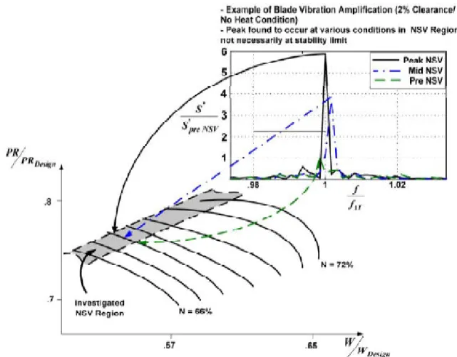
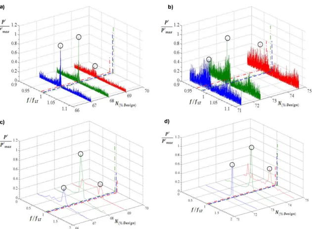
Figure 2.8 : Near stall NSV region and vibration amplification as experimentally observed by Thomassin et al. (2008) ... 19 Figure 2.9 : Measured instability convection coefficient (k), Thomassin et al. (2008) ... 20 Figure 2.10 : Frequency spectrum of unsteady blade pressure: measured for a) cold and b) hot T1
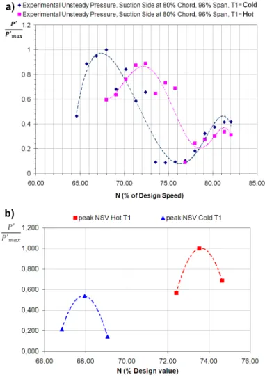
and calculated for c) cold and d) hot T1, both plotted vs rotor speed ... 22 Figure 2.11 : Peak amplitude of unsteady blade pressure a) measured and b) calculated at 80%
chord, 96% span for both cold and hot inlet temperatures ... 23 Figure 2.12 : Numerical vs experimental predictions of the convection velocity (UF) shown for a)
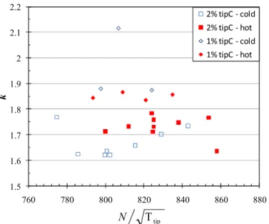
resonance condition and b) tip instability convection coefficient ... 24 Figure 3.1 : Measured instability convection coefficient, k, at different operating conditions, data
from Thomassin et al. (2008) ... 29 Figure 3.2 : Detailed mesh for Subsonic Rotor (SR): a) side view, b) blade tip section, c) span cut
at mid-chord and d) close-up view of tip region ... 32 Figure 3.3 : Detailed mesh for Transonic Rotor (TR): a) side view, b) blade tip section, c) span
cut at mid-chord and d) close-up view of tip region ... 33 Figure 4.1 : Typical chord-wise VL profiles calculated at different speeds for a) SR geometry at
1% chord tip clearance and b) TR geometry at 0.4% chord tip clearance ... 37 Figure 4.2 : Calculated tip leakage velocity profiles at 20% chord for a) SR geometry (N=70%)
and b) TR geometry (N=71%) ... 39 Figure 4.3 : Area-averaged turbulent kinetic energy at tip averaged for all speeds with logarithmic
trend lines (dashed lines) ... 40 Figure 4.4 : a) Profile transition and b) detailed velocity profiles as tip clearance is increased, c)
model of equation (4.3) derived based on velocity profile transitions ... 41 Figure 4.5 : Calculated k, a) Overall results, b) Comparison of available data in the literature with
xxiv
Figure 4.6 : a) Distorted velocity profiles calculated at 20% chord and 3.83% tip clearance for the SR geometry, b) Ideal tip clearance flow model of Rains (1954) as depicted in Storer and Cumpsty (1991) and c) vena-contracta as observed in simulations for N=74% in a) ... 44 Figure 4.7 : Calculated k at different inlet temperatures near stall for the TR geometry.
Experimental data is from Thomassin et al. (2008) ... 45 Figure 4.8 : Calculated blade loading vs. non-dimensional tip clearance for both SR and TR
geometries (data shown for all the different speeds) ... 47 Figure 4.9 : a) Equation (4.8) and b) its derivative plotted vs ψ ... 49 Figure 4.10 : Typical values of loading, ψ, and flow coefficient, φ, found near stall for different
compressor geometries available in the literature ... 50 Figure 5.1 : Possible configuration for choke NSV, a) chord-wise profile of speed-averaged VL/Ca
in choked flow conditions showing jet-like pattern near trailing-edge and b) vector plot at tip showing impingement near trailing edge, data calculated for TR geometry, N=82% and 1.29% tip clearance ... 56 Figure A2.1 : Details of compressor rig installations ... 62 Figure A2.2 : Overview of PIV equipment and installations ... 63 Figure A2.3 : Detailed view of PIV installations, a) close-up view of field of view and laser sheet
delivery lense and b) detailed view of the calibration system ... 64 Figure A2.4 : CAD view of PIV experiment: a) detailed view of test-section and b) co-radial PIV
measurement planes shown in % blade span ... 65 Figure A2.5 : Example of PIV experimental results obtained at sea-level conditions for N=68%
design measured at a) 98%, b) 96% and c) 94% blade span co-radial planes. Shown in d) is equivalent numerical results calculated at 99% span co-axial plane. ... 66 Figure A3.1 : TR geometry - Chord-wise VL profiles calculated at different speeds and tip
clearances ... 81 Figure A3.2 : SR geometry - Chord-wise VL profiles calculated at different speeds and tip
Figure A3.3 : TR geometry - Calculated tip leakage velocity profiles (span wise) at different speeds and tip clearances ... 83 Figure A3.4 : SR geometry - Chord-wise VL profiles calculated at different speeds and tip
xxvi
INITIALS AND ABBREVIATIONS
A Blade tip displacement amplitude [m]
c Local speed of sound [m/s] Ca Mean axial velocity [m/s] CFD Computational Fluid Dynamics
Cp Specific heat at constant pressure [kJ/(kg-K)]
D Diameter [m]
EO Engine Order (1,2,3,...)
f Frequency [Hz]
FIV Flow-induced vibrations FOR Frame of reference h Tip clearance size [m]
k Tip instability convection coefficient (Utip/UF)
L Length or distance [m]
LE Leading edge
M Mach number
n Harmonic integer number
N Rotational speed [rpm] NSV Non-Synchronous Vibrations
p’ Pressure fluctuation, unsteady pressure [Pa] PIV Particle Image Velocimetry
PR Pressure ratio
PS Pressure side
RI Rotating Instabilities
s Blade pitch (inter-blade) distance [m] S’ Vibration level [Pa]
SS Suction side
St Strouhal number (reduced or non-dimensional frequency) T Torsional vibration mode, Temperature [K]
TE Trailing Edge
U Flow velocity [m/s]
Utip Blade tip velocity [m/s]
UF Foward wave (jet) speed [m/s]
VL Tip leakage flow velocity [m/s]
W Air mass flow [Kg/s]
Wcorr Corrected air mass flow (Wcorr = W*√[(T/Tref)/(P/Pref)]) [Kg/s]
Greek symbols
α Absolute air flow angle [deg.], Correlation coefficient β Relative air flow angle [deg.], Correlation coefficient γ Specific heat ratio
η Compressor efficiency
θ Temperature ratio (inlet temperature/reference temperature) [T1/Tref]
λ Wave length [m]
µ Dynamic viscosity [Pa.s]
ξ Hub-to-tip ratio
xxviii
σ Tip solidity (ςtip/s)
ς Chord length [m]
τ Non-dimensional tip clearance (τ = h/ςtip)
φ Flow coefficient
ψ Loading coefficient, pressure coefficient ω Angular frequency [rad/s]
Subscripts
0 Local, total
b Blade
B Backward wave in rotating frame c Speed of sound, critical
D Diameter [m], Design
F Forward wave in rotating frame
h Hub
j Jet
max Maximum
min Minimum
LIST OF APPENDICES
APPENDIX 1 – Particle Image Velocimetry (PIV) Experiment ... 62 APPENDIX 2 – GT2009-59074: Numerical Investigation into Non-Synchronous Vibrations of Axial Flow Compressors by the Resonant Tip Clearance Flow ... 69 APPENDIX 3 – Additional Numerical Results ... 81
1
CHAPTER 1
INTRODUCTION
The gas turbine industry has been one of the few technological sectors that have shown continuous and sustained research and development since its early debut in the mid 1900’s. Nowadays, modern gas turbine companies are pushing the design to the limits in terms of thrust-to-weight ratio and specific fuel consumption, in order to thrive in the competitive market. This war on weight has led to new challenge in terms of vibrations of the diverse gas turbine engine components. Being able to understand and master the numerous vibration phenomena, often associated with fatigue damage of components, thus represents a tremendous competitive advantage on the market. The current work will focus on vibrations encountered in the axial compressor module found in modern gas turbine engines, more specifically, Non-Synchronous Vibrations (NSV). Although some relevant details on compressor will be given, it will be assumed throughout this work, that the reader has some basic knowledge on the subject.
1.1 Review on Axial Flow Compressors
1.1.1 Flow Features and Operating Principle
An axial compressor involves two main components, the rotor that accelerates the flow and that is essentially made of a disc with a number of airfoils, referred to as “blades”, which rotates confined within a casing. The second main component is the stator, that converts the kinetic energy into static pressure rise, and is also made of a disc with airfoil sections but that are fixed with respect to the rotor. Typically, many stages are required to achieve the desired pressure rise through the compressor module. An illustration of a typical compressor stage (rotor and stator) assembly is shown for reference in Figure 1.1. This configuration leads to an important and widely studied aspect of compressor aerodynamics, namely the tip clearance flow, which is the air that flows through the spacing between the rotor blade tip and the casing, as shown also in Figure 1.1. Typically, the tip clearance size in commercial gas turbine engine is on the order of 1% of the blade tip chord.
Figure 1.1 : Typical axial compressor stage configuration
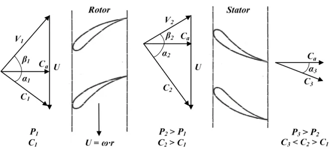
Figure 1.2 shows the typical flow features of an axial compressor stage. The velocity triangles are used to determine the magnitude and direction of velocity vectors through the stage. The velocity component and direction in the blade frame of reference are denoted V and β, respectively, while the velocity component and direction in the absolute frame of reference are identified by C and α, respectively. The subscripts 1, 2 and 3 are referring to the inlet, mid-stage and outlet locations, respectively. In addition, Ca is the axial velocity component and U is the rotor blade speed at a
3
Figure 1.2 : Flow features of a typical axial compressor stage (rotor and stator)
The operating principle of an axial compressor was briefly described previously. As shown in Figure 1.2, the rotor accelerates the air while providing some static pressure increase, resulting in
P2>P1 and C2>C1. The air then flows through the stator where the kinetic energy of the fluid is
converted into static pressure rise, by deceleration of the flow, which results in P3>P2 and
C3<C2>C1. The fraction of static pressure rise provided by the rotor, when compared to the total
pressure rise in the stage, is called the “degree of reaction” and is typically on the order of 0.5. This means that the rotor and stator are sharing approximately half of the static pressure increase through the stage.
1.1.2 Performance and Characteristics
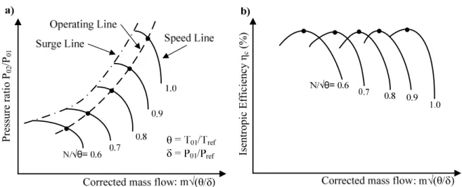
The performance of axial compressor is typically characterized in terms of pressure ratio and efficiency. Figure 1.3 (a) shows a “compressor map” which is a plot of the stage pressure ratio versus the corrected mass flow. The surge line identified on the figure corresponds to the point of compressor stall or reverse flow while the operating line corresponds to the operating point of maximum efficiency. The speed lines are also identified which are points along a constant corrected speed (N/√θ) and are shown as a fraction of the design speed in the figure. Figure 1.3 (b) shows the isentropic efficiency, also plotted as a function of the corrected mass flow where the point of maximum efficiency are identified and corresponds to the operating line points on Figure 1.3 (a).
Pr es su re r at io P02 /P01 Is en tr op ic E ff ic ie nc y ηc (% )
Figure 1.3 : Axial compressor characteristics, a) Pressure ratio and b) Efficiency vs corrected mass flow
1.1.3 Tip Clearance Flow Features
As it was previously mentioned, the typical configuration of axial flow compressors leads to an intrinsic feature of compressors: the tip clearance flow. The tip clearance flow is an air flow that is pressure driven (aerodynamic loading) which flows through the spacing between the rotor blade tip and the casing, as previously depicted in Figure 1.1. The principal features and characteristics of the tip clearance flow are shown in Figure 1.4 (Vo, H.D., 2001), for high aerodynamic loading conditions. In such conditions, the high incidence of the incoming flow leads to flow separation near the blade tip which creates a vortex, called the “tip clearance vortex”, that is the results of fluid mixing between the separated flow and the tip clearance flow. This also leads to a passage blockage that increases in size as the aerodynamic loading increases.
5
Figure 1.4 : Basic tip clearance flow features (Vo, H.D., 2001)
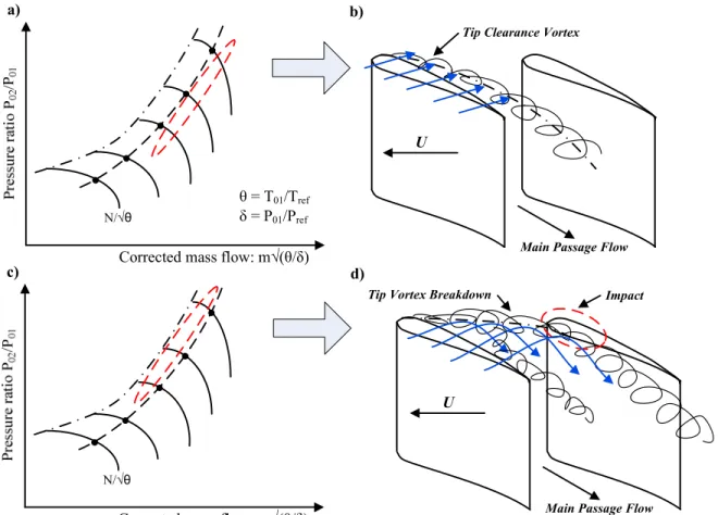
Figure 1.5 also depicts the behavior of the tip clearance flow as the aerodynamic loading is increased. In Figure 1.5 (a), a region of moderate aerodynamic loading, located just before peak efficiency or operating line, is circled by a dashed line. In such conditions, the tip clearance vortex is relatively small in size, as shown in Figure 1.5 (b), since the angle of incidence of the incoming flow is moderate. In addition, the tip vortex is redirected in the stream-wise direction by the high momentum incoming flow. In conditions of high aerodynamic loading, such as in conditions near stall as shown in Figure 1.5 (c), the angle of incidence of the incoming flow at the blade tip is such that the tip vortex is now bigger in size. It has more momentum than the incoming flow in the tip region such that it evolves tangentially and eventually travels across the passage and impact on the upcoming blade, as illustrated in Figure 1.5 (d). In some cases, the tip vortex is divided in two distinct portions, which are no longer “vortex” (strictly speaking), as a vortex core cannot usually be identified. This is also identified in Figure 1.5 (d) where a portion of the broken tip vortex follows the first blade suction side while another follows the upcoming blade pressure side.
N/√θ
Corrected mass flow: m√(θ/δ)
c)
Main Passage Flow
U
Tip Vortex Breakdown
Main Passage Flow
U
Impact
d)
N/√θ
Corrected mass flow: m√(θ/δ) θ = T01/Tref δ = P01/Pref
a) b)
Tip Clearance Vortex
Figure 1.5 : Characteristics of the tip clearance flow at moderate aerodynamic loading in (a) and (b) and high loading near stall in (c) and (d)
1.2 Vibrations in Axial Flow Compressors
Compressors are prone to vibrations which are generally categorized as mechanical vibrations, originating from mechanical interaction among the diverse engine components, and flow-induced vibrations (FIV) that are often the result of a fluid-structure interaction between the rotor blades and the air flow through the compressor. The flow-induced vibration category is typically divided in two distinct sub-categories, which are “forced response” and “fluid-elastic instabilities”. The latter includes classical flutter and non-synchronous vibrations (NSV). The various types of vibrations are depicted on the Campbell diagram, shown here in Figure 1.6, which is the tool that is typically used to consider vibration sources in compressor design. The latter has on the abscise axis, the rotational speed of the rotor shaft, and on the ordinates axis, the frequency of excitation. The natural frequency modes of the blade are plotted, on the Campbell diagram, as a function of the rotational speed and show a slightly positive slope due to the inertial force that increases as
7
the speed increase, which changes the blade stiffness resulting in a change in the blade natural frequency.
Figure 1.6 : Different vibration types depicted on the Campbell diagram
The forced response vibrations are the most typical vibrations sources in compressors and are known to be “synchronous” with the rotational speed of the shaft. This means that the frequency of excitation will be an integral multiple of the frequency of the rotational speed, known as “engine order” (EO). Typical sources of EO forced excitation are the blade wakes of the upstream blade row as well as the potential excitation of the downstream blade row. Coincidence of the frequency of excitation with one of the blade mode will results in a forced vibration of the blade. Unevenly distributed wakes coming from the stator can also results in sub- or super-harmonics of the engine order, resulting in 2EO, 3EO, etc excitation frequencies.
The fluid-elastic vibrations, on the other hand, are not necessarily synchronous with the rotor speed, as opposed to forced vibrations. A typical type of fluid-elastic instability that is of major concern in compressor design is known as “flutter”. Classical flutter is the most common and understood type of flutter and consist of exponentially growing vibrations when the “flutter speed” is reached; meaning that the only way out of classical flutter is to go down in rotor speed below the flutter speed. This is very distinctive from NSV which occurs through a resonance despite that both phenomena can occur at non-integral multiple of the rotor speed. In addition,
many different types of flutter have been reported in the industry (Dowell, E.H., Crawley, E.F., Curtiss Jr, .H.C., Peters, D.A., Scanlan, R.H. and Sisto, F., 1995) and have often been a source of confusion with NSV. This is also why NSV cases have been vaguely reported in the last 15-20 years.
1.3 Research Objectives
Thomassin, J., Vo, H.D. and Mureithi, N.W. (2008, 2009) have proposed a mechanism and a model to explain the physics behind NSV. The latter was statistically and experimentally proven to be a powerful tool to predict the critical rotor speed at which NSV are likely to occur. However, the model was found very sensitive to what was defined as the “instability convection coefficient” (k) by Thomassin et al. (2008). In fact, the initial approximation of k=2 in the model (Thomassin et al., 2009) also showed significant error (up to ~20%) in the NSV predictions, which can only be improved by complex experimental measurements to determine the actual “k”, as performed by Thomassin et al. (2008). The general objective of the research work described herein is to use computational fluid dynamics (CFD) to improve the NSV prediction model and extend our comprehension of the physics behind NSV. More specifically, the objectives are:
1. Estimate the “k” parameter from numerical simulations and determine how the tip clearance size and operating temperature affect its value.
2. Propose a correlation for “k” that can be used as a complementary tool to the NSV model proposed by Thomassin et al. (2008, 2009) such that the critical NSV speeds can be assessed in the very early design stage, independently from numerical simulations and experiments.
3. Assess the generic nature of the study by looking at the relevant fluid mechanics and aerodynamic characteristics of axial compressors and address the possibility to encounter NSV in choked-flow conditions, as opposed to the near-stall region where NSV are known to occur.
9
1.4 Thesis Organization
A brief introduction on compressor vibrations and the main objectives of the current work were presented in the introduction of chapter 1. Chapter two presents an historical background and literature review on NSV, along with a detailed description of the NSV model proposed by Thomassin et al. (2008, 2009). The relevant details of the work from Drolet et al. (2009) that led to the present thesis are also summarized in chapter 2. Chapter 3 describes the details of the methodology used for the current work. Chapter 4 presents the results of simulations that were conducted to assess the effect of tip clearance size and operating temperature on the k parameter involved in the critical NSV prediction model of Thomassin et al. (2008) (specific objective 1). It also proposes a correlation for k, based on the numerical results, that improves the critical NSV speed predictions using the proposed model and discusses the generic nature of the study (specific objective 2 and part of specific objective 3). Chapter 5 summarizes the main conclusions and contributions of the work described herein and also discuss on recommendations for future work, based on the results and observations presented in the current thesis (specific objective 3).
1.5 Research Contributions
This study proposes a correlation for the instability convection coefficient (k) that significantly improves the critical NSV speed predictions. The proposed correlation was also proven to be generic for any given compressor geometry. In addition, this work suggests a possible configuration for NSV to occur in choked-flow conditions as a recommendation for future work.
CHAPTER 2
LITERATURE REVIEW
This chapter presents a literature review on Non-Synchronous Vibrations (NSV) observed in axial flow compressors. First, an historical background on the subject is presented along with main contributions from previous research work. Secondly, a model that was proposed to predict the critical blade tip speed at which NSV can occur is presented in greater details since the current thesis builds upon this specific work. Finally, a numerical method that was developed to refine the critical NSV speed predictions is presented as the current research is also a direct continuation from this previous numerical work.
2.1 Background on Non-Synchronous Vibrations
One of the first reported NSV cases in the industry is attributed to Baumgartner M., Kamaler F. and Hourmouziadis J. (1995). They have linked NSV with rotating instabilities (RIs) from experimental observations. Rotating instabilities can be described as an oscillating flow phenomenon that causes periodic vortex separation and axial reverse flow in the tip clearance region (Mailach et al., 2001a) and were widely studied in the past as a possible excitation source for compressor blades. Examples can be found in Liu, J.M., Holste, F., Neise, W., 1996; Kameier, F. and Neise, W., 1997a; Kameier, F. and Neise, W., 1997b; Mailach, R., Lehmann, I. and Vogeler, K., 2001a; Mailach, R., Sauer, H. And Vogeler, K., 2001b; März, J., Hah, C. and Neise, W., 2002. RIs were associated with high amplitude vibrations and noise generation on compressor rotor blades. They were also modeled as a noise source or pressure fluctuation (p=p(t)), as shown in Figure 2.1, emanating from the leading edge tip vortex, possibly linked with NSV.
In fact, an interaction between the leading edge tip vortex and the adjacent blade was found by März et al. (2002), Fukano, T. and Jang, C.M. (2004) and Zhang, H., Lin, F., Chen, J., Deng, X. and Huang, W. (2006). Figure 2.1 depicts the different models that were proposed for rotating instabilities by a) Baumgartner et al. (1995) and b) Mailach et al. (2001). Kameier and Neise (1997a) have also found a Strouhal number (reduced frequency) for rotating instabilities that was function of the tip clearance and aerodynamic loading. This Strouhal number was later refined by Mailach et al. (2001) and found to be a constant at given flow conditions and blade geometry.
11
a)
b)
Figure 2.1 : Models proposed for rotating instabilities (RI) by a) Baumgartner et al. (1995) and b) Mailach et al. (2001)
It was not before 2003 that rotating instabilities, similar to that studied by Baumgartner et al. (1995), were named “non-synchronous vibrations” (NSV) by Kielb, R.E., Thomas, J.P., Barter, J.W. and Hall, K.C. (2003) who experimentally identified the effect of operating conditions, such as temperature, on NSV and linked it with tip clearance flow instabilities through numerical simulations. They have also observed a sudden step change in the frequency mode associated with NSV, for constant operating conditions, which is one of the most distinctive features of NSV. Later, Vo, H.D. (2006) found that the trailing edge backflow of tip clearance fluid, which is
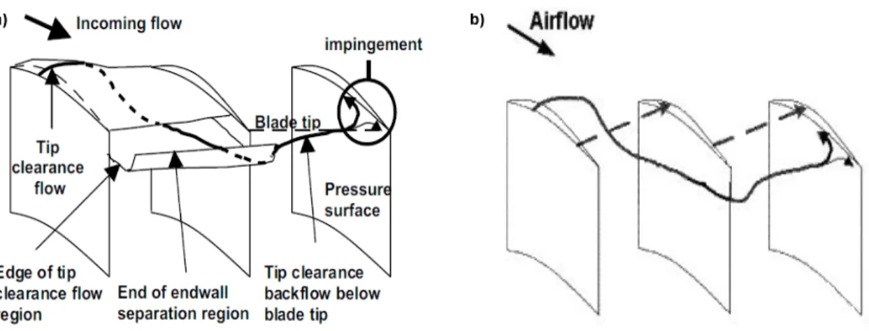
one of the criteria for spike-initiated rotating stall (Vo, H.D., Tan, C.S. and Greitzer, E.M., 2008), showed signs of impingement on the upcoming blade, as shown in Figure 2.2 (a). This phenomenon occurs near stall and thus, at high aerodynamic loading. These observations were also experimentally observed later by Deppe, A., Saathoff, H. and Stark, U. (2005). Vo, H.D. (2006) also suggested, based on his observations, that the dynamics of impinging jets could possibly explain the underlying physics behind NSV.
Figure 2.2 : Proposed tip clearance flow impingement patterns, possibly the physical mechanism behind NSV, from a) Vo (2006) and b) Thomassin et al. (2008)
2.2 Proposed Theory on Non-Synchronous Vibrations
In light of the proposed impinging jet analogy, Thomassin, J., Vo, H.D. and Mureithi, N.W. (2009) have reviewed the dynamics of impinging jets in order to explain the physics behind non-synchronous vibrations. They developed a novel theory for resonant impinging jets at Mach numbers of similar magnitude to those typically found in tip clearance flows of axial compressors. Based on their theory, a physics-based model was derived to predict the compressor blade tip speeds at which NSV are most likely to occur (Thomassin et al., 2009). The model was also experimentally verified by Thomassin, J., Vo, H.D. and Mureithi, N.W. (2008). The research presented in this thesis builds on previous work from Thomassin et al. (2008, 2009). Hence, this section presents their findings in greater details to help the comprehension of the reader throughout the current work.
13
2.2.1 The Jet Core Feedback Theory
Ho, C.-M. and Nosseir, S. (1981) studied the dynamics of high-speed subsonic jets impinging on rigid flat plates. They found that the shear layer emanating from the jet lip produces vortical structures that are convected at approximately half of the jet velocity and that scales with the jet diameter (D) and mean velocity (U). These turbulent structures create acoustic reflections that propagates outside the jet potential core when impinging on a rigid plate that is located in the jet potential core (typically L ≈ 7 D, where here L is the jet-to-plate distance corresponding to the extent of the jet potential core). When the reduced frequency, or Strouhal number (St = fD/U),
reaches a critical value such that the acoustic feedback wavelength corresponds to the jet-to-plate distance, there is a significant amplification of the pressure fluctuation on the plate. In such conditions, the jet is said to be “resonant”. Examples of a resonant and non-resonant jet are shown in Figure 2.3 (a). Typically, the lowest Mach number at which a jet can become resonant, when impinging on a rigid plate, was found to be 0.65, as shown in Figure 2.3 (b) from Lucas, M.J. (1997). Although the analogy of a jet impinging on a plate, as proposed by Vo (2006), looked promising, the Mach numbers observed in compressor tip clearance flows are typically lower than M=0.65.
Figure 2.3 : a) Response of a jet impinging on a rigid plate: resonant jet at M=0.8 and non-resonant jet at M=0.5, from Ho et al. (1981) and b) reduced frequency (Strouhal number) range