Systems : Application to Parallel Manipulators
J.-F. COLLARD1, P. FISETTE1 and P. DUYSINX2
1Universit´e Catholique de Louvain, Center for Research in Mechatronics, place du Levant, 2, B-1348 Louvain-la-Neuve, Belgium;
2Universit´e de Li`ege, D´epartement ProM´eTh´e, chemin des Chevreuils, 1, Bˆat B52, B-4000 Li`ege, Belgium
March 1, 2004
Abstract. This paper describes an original and robust method to optimize the de-sign of closed-loop mechanisms, especially parallel manipulators. These mechanisms involve non linear assembling constraints. During optimization, the Newton-Raphson algorithm we use to solve these constraints may fail when the Jacobian matrix of the constraints is ill-conditioned and stops the redesign process. To circumvent the difficulty, the technique we propose takes advantage of numerical conditioning to penalize the objective function. Applications to an academic example and parallel robots demonstrate the capabilities of the methodology.
Keywords: design optimization, penalty, closed-loop multibody systems, parallel manipulators
1. Introduction
Most of present issues in the field of multibody system (MBS) dynamics involve other scientific disciplines to enlarge and enrich the results of the MBS analysis. Combining multibody analysis and optimization tech-niques has sometimes been exploited in the literature (e.g. : [1, 2, 3]), but the few existing results are still not able to cope completely with some limitations and/or conflicts. Several issues are addressed in recent researches: applicability of optimization methods for some families of MBS, problem formulation in terms of cost function, especially for constrained systems, computer efficiency and parallel computation al-gorithms, etc. However, current researches mainly produce guidelines rather than rigid rules regarding the coupling of multibody dynamics and optimization in a particular context, i.e. a family of applications and a given type of objective function. As examples, one can cite the optimal design of a vehicle transmission [1], of 3D manipulators [4, 5, 6, 7, 8], the optimal synthesis of mechanisms [2, 9, 10] and parallel robots [11, 12, 13] as well as the optimization of suspension and railway vehicle [3, 14, 15], or machine tools [16].
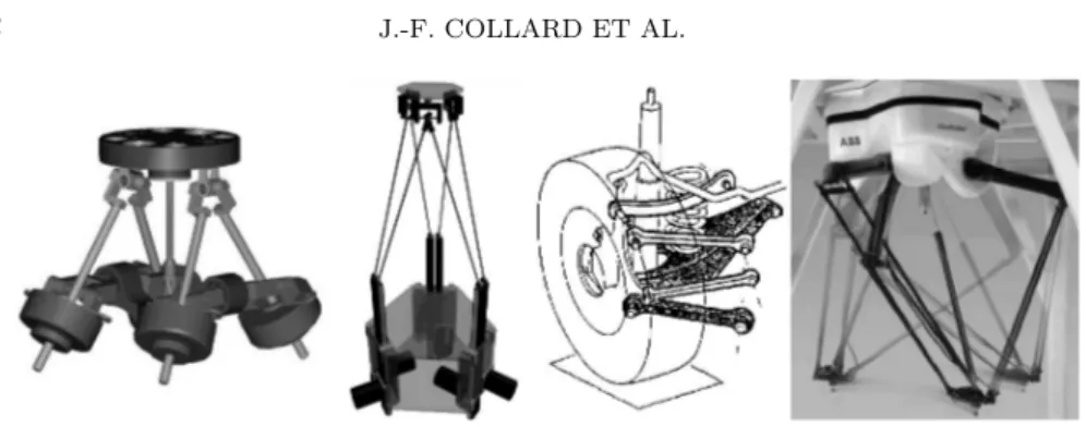
Figure 1. Examples of closed-loop mechanisms
The present research tackles the optimization problem of MBS con-taining three-dimensional kinematic loops as shown in Figure 1, involv-ing :
• geometrical design parameters;
• a single scalar objective function whose nature may be geometrical, kinematic or dynamical.
In this case, the question that is addressed is the following: how to build a robust cost function for those systems such that a classical optimization method can iterate with good convergence properties and without troubleshooting in terms of loops closure (or “system assem-bling”) ? For simple systems, one can obviously circumvent the problem by expressing explicitly some optimization constraints on the geometri-cal parameters (length of segments, amplitude of motion, etc.), but, as soon as complex multi-loop systems like 3D parallel manipulators are involved, this is not possible anymore. The original approach that is used here is based on a penalty technique in which unreachable config-urations (i.e. configconfig-urations where it is not possible to assemble or to actuate the mechanism) and design constraint violations are avoided by a large cost of the objective function. The proposed method extends the parameter space and thus the cost function definition domain beyond the feasible and assembly domain, leading to a continuous and well-defined cost function. Hence, this allows to use efficient unconstrained optimization methods as BFGS method, Nelder-Mead Simplex, etc. . .
The approach will be illustrated at first on the basis of a quite aca-demic example: the design optimization of a planar ejector to improve dynamical performances. Then the method will be applied on more realistic problems: the dexterity optimization of a parallel manipula-tor – the Hunt platform – to enhance kinematic performances. More precisely, the goal is to maximize the average robot isotropy over a workspace cube with respect to geometric design parameters.
2. Optimization and Assembling Constraints
Before expressing the limitations due to assembling constraints, we will briefly describe the multibody formalisms we use to compute the inverse and direct models of constrained MBS which are generally involved in the computation of the objective function. Indeed, it is important to know the origin of these assembling constraints in the case of closed-loop mechanisms. MBS dynamical formalisms will be described first. Main issues due to assembling constraints will be explained thereafter. 2.1. MBS dynamical formalisms
Most multibody applications contain loops of bodies (car suspension, parallel robots, mechanisms, etc. . . ) which force the generalized coor-dinates q – relative joint coorcoor-dinates in our formalism – to satisfy m geometrical constraints h(q) = 0 at any time. In order to fully describe the system, these assembling constraints and their first and second time derivatives must be added to the equations of motion, in which constraint forces are introduced via the Lagrange multipliers technique:
M (q) ¨q + c(q, ˙q, fext, text, g) = Q(q, ˙q) + Jtλ (1)
h(q) = 0 (2)
˙h(q, ˙q) = J(q) ˙q = 0 (3)
¨h(q, ˙q, ¨q) = J(q)¨q+ ˙J ˙q(q, ˙q) = 0 (4) where:
• M [n ∗ n] is the symmetric generalized mass matrix of the system, • q [n ∗ 1] denotes the relative – or joint – generalized coordinates, • c [n ∗ 1] is the non linear dynamical vector which contains the
gy-roscopic, centrifugal and gravity terms as well as the contribution of components of external resultant forces fextand torques text,
• Q [n ∗ 1] represents the generalized joint forces (torques).
• J = ∂q∂ht denotes the constraint Jacobian matrix (dimension: [m ∗
n]),
• J ˙q(q, ˙q) [m ∗ 1] is the quadratic term (expression in ˙q˙ i ˙qj) of the
constraints at acceleration level (dimension: [m ∗ 1]),
• λ represents the Lagrange multipliers associated with the
Various methods can be used to solve the system (1–4), i.e. to predict the motion of the system (q(t), ˙q(t)), starting from an initial configuration (q(t = 0), ˙q(t = 0)), by time-integrating the accelerations
¨
q(t). Amongst these, one can opt for a full reduction of the system to
a purely differential form, which can be obtained by means of the
Co-ordinate Partitioning [17]. Assuming that the constraints h(q) = 0 are
independent and after reordering the vector of generalized coordinates
q (and the columns of the constraint Jacobian J accordingly), we can
perform the following partition:
q = µ u v ¶ ; J =¡Ju Jv ¢ (5)
where u denotes the subset of (n − m) independent coordinates and v denotes the subset of m dependent coordinates. By correctly1 choosing
the subset v, the m by m matrix Jv will be regular.
Once the coordinate partitioning is established, the reduction method simply uses matrix permutations and operations to produce the equa-tions of motion in ODE form. Let us first partition the generalized mass matrix M and the vector c according to the coordinate partitioning (5):
µ Muu Muv Mvu Mvv ¶ µ ¨ u ¨ v ¶ + µ cu cv ¶ = µ Qu Qv ¶ + µ Jut Jvt ¶ λ (6)
When Jv is regular, eliminating the unknowns λ using the lower part of system (6) produces: ¡ Muu Muv¢ µ ¨ u ¨ v ¶ +Bvut ¡ Mvu Mvv¢ µ ¨ u ¨ v ¶ +cu+Bvutcv = Qu+BtvuQv (7) where we define the so-called coupling matrix Bvu, − (Jv)−1Ju.
Then using the first (eq. (3)) and second derivatives (eq. (4)) of the constraints, the generalized velocities and accelerations ˙v and ¨v are
respectively given by:
˙v = Bvu˙u (8)
¨
v = Bvuu + b with b , −J¨ v−1( ˙J ˙q) (9)
and can also be eliminated from the differential equations (7). This produces the final reduced ODE system, concisely written as:
M(u, v)¨u + F( ˙u, u, v) = Q( ˙u, u, v) (10)
where Q denotes the joint generalized forces (torques) associated with the actuated2 joints. From this system, direct (¨u = M−1(Q − F)) and
inverse3 (Q = M¨u + F) dynamic formulations may be easily extracted.
The algebraic constraints still have to be solved in order to elim-inate the dependent variables v from (10). While analytical solutions can exist for specific cases, general algebraic constraints (2) require a numerical procedure to be solved: the Newton-Raphson iterative algorithm can be used for successive estimations of v:
vk+1= vk− (Jv)−1h |v=vk (11)
where the right hand side is evaluated for v = vk and the values of u
corresponding to the instantaneous system configuration.
Thanks to this final numerical elimination, the set of purely differ-ential equations (10) constitutes the equations of motion of the con-strained system described in terms of the n−m independent generalized coordinates u.
2.2. Main issues due to assembling constraints
In some cases, we may face convergence problems of the Newton-Raphson algorithm to solve the constraints (11) and such problems can be frequently encountered when performing a geometrical optimization process.
a. Multiple solutions b. Singularity:
¯ ¯ ¯∂v∂ht ¯ ¯ ¯= 0 c. Impossibility: h(u, v) 6= 0, ∀v Figure 2. Troubleshooting cases when solving assembling constraints
• A first case may occur when the solution in term of v is not unique
for a given vector u (see Figure 2.a). A way to prevent from that is to start the algorithm with initial values close to the expected solution.
2 Which do not necessary coincide with the independent joint coordinates u. 3 In practice, inverse dynamics does not require the explicit computation of the mass matrix (O(N2) complexity). An O(N ) recursive formalism is used to get Q more straightforwardly.
• A second problem may happen if the mechanism reaches a singular
configuration, the constraint Jacobian matrix Jv = ∂v∂ht becoming
singular4 (see Figure 2.b). Practically, those singularities
corre-spond to a loss of mobility of the robot by locking one or more actuators associated with joint variables u. They can be assimi-lated to unreachable points in the parameter space. Therefore, the cost function will be penalized at that point, even if it is possible to close the mechanism by another choice of the partitioning.
• Finally, it can be impossible to close the mechanism simply because
a constraint hihas no root: the Newton-Raphson algorithm cannot
converge towards a solution (see Figure 2.c). In that case, the closed mechanism doesn’t exist but, instead of rejecting it, we will keep it and penalize the cost function accordingly.
In the optimization process, the second and third cases will be treated in the same way, as explained in the next section. For the first case, we rely on the robustness of the Newton-Raphson process when iterating from a neighborhood of a well-known closed configuration. Other configurations are found by small increment around and from the latter: by experience, this technique is reliable and ensures a robust convergence in any case.
Let’s point out that the penalization of the cost function which is caused by unsatisfied geometrical constraints may occur whatever is the nature (geometrical, kinematic or dynamical) of the cost function itself.
3. Penalty Optimization Method
3.1. How to Extend the Objective Function outside the Closed-Loop Domain ?
In order to perform a smooth penalization of the objective function
f (P ), it is important to find the closed-loop border according to the u, v partitioning in the parameter space. The idea here is to observe
the conditioning of the constraint Jacobian matrix Jv which indicates
4 Two kinds of singularities are considered here: the mathematical singularities, arising from a wrong choice of the sequence of rotation variables, and those associ-ated with ignorable variables such as the axial rotation of a connecting rod. They can be avoided by achieving a suitable model of the mechanism.
the proximity of that border where the determinant of Jv vanishes to zero5.
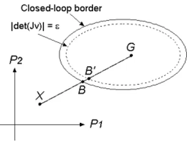
Let’s take an application with two parameters P1,P2 (see Figure 3).
Let’s suppose that the optimizer is calling the objective function – assumed to be scalar – outside the closed-loop border, at point X. Then a fixed point G is chosen inside the boundary6 and the penalization is computed along the direction GX from a point B0. The latter is located
close to the border, where the absolute value of the determinant of Jv reaches a threshold ² (strictly greater than zero), to avoid singular con-figurations and numerical round-off problems. The closed-loop border is for instance detected on the basis of the number iter of iterations of the Newton-Raphson algorithm which reaches the maximum iterM7.
Figure 3. Penalization along direction GX
The search of B0 is simply done by a dichotomic search along the
segment [G, X] (see Figure 3). Various cases are considered:
• The Newton-Raphson algorithm converges: iter < iterM ⇒ [B, G]
seg-ment:
• |det(Jv)| ≥ ² ⇒ [B0, G] segment
• |det(Jv)| ≤ ² ⇒ [B0, B] segment
• The Newton-Raphson algorithm doesn’t converge: iter ≥ iterM ⇒
[B, X] segment
Once point B0has been found and f (B0) has been evaluated, we suggest
to compute and penalize f (X), on the basis of f (B0). This extension
may be continuous or not, the only condition is to make sure that 5 The present approach is clearly partitioning-dependent. A way to circumvent this limitation should be to consider all the possible coherent partitioning to find the border proximity in the parameter space.
6 Various possibilities can be envisaged to choose point G: for instance, the last update of the optimal parameter values.
7 Typically, iter
f (X) > f (B0). In the proposed examples, different kinds of extension
have been applied and a rather simple algorithm has been used: the Nelder-Mead simplex method, which is robust but slowly convergent.
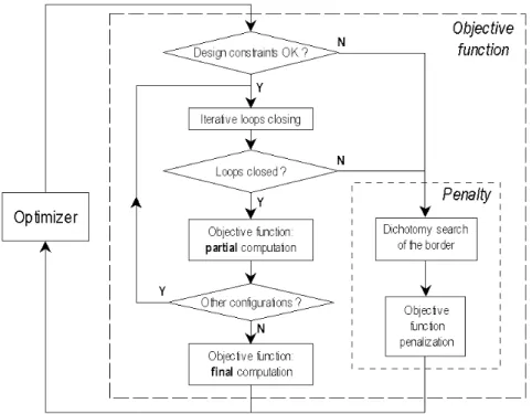
3.2. The Objective Function Algorithm
The optimization procedure flowchart is given in Figure 4.
Figure 4. Objective function computation algorithm
Each time the optimizer calls the objective function, design con-straints8 imposed by the designer are evaluated first. If they are
sat-isfied, the mechanism can be assembled using the Newton-Raphson algorithm described before. If the latter converges, the objective func-tion which involves that configurafunc-tion (or a set of configurafunc-tions, as in the application section 5.2) can be evaluated. Otherwise, if one of both tests is unsatisfied, the penalization process9 begins: first, the border
is found by the dichotomy method as explained before and then, the objective function is extended continuously and returns a penalized
8 e.g. : upper or lower bound of a parameter.
9 Up to now, we systematically deal with the design constraints in the same way as the closed-loop constraints, using the same penalty approach.
value to the optimizer. However, in some cases, if an upper bound of the objective function is known, it may be quickly extended discontinuously without searching the border10.
4. First Example: Design of a Planar Ejector
The system (see Figure 5.a) consists of two bodies: a ball (radius: R = 7 cm, mass: M = 300 g) and a simple articulated arm (negligible mass) which has to push the ball with a torque QP over a distance L = 20 cm,
slope: α = 30◦. The problem was stated in the frame of a mobile robotic
project for which such an ejector had to be designed. The contact point
S is supposed to be fixed on the right arm tip thanks to a roller (whose
axial rotation is disregarded). This first - quite academic - example can thus be modelled as a slider-crank mechanism (see Figure 5.b) whose optimization parameters are the position (x, z) of the joint P and the length of the crank k−→P Sk = l (k−→CSk = R). All the coordinates are
expressed in the inertial frame {O, ˆI1, ˆI3}, where O is located at the
origin of the ball movement.
a. Planar ball ejector. . . b. . . . modelled by a slider-crank mechanism Figure 5. Planar ejector model
Two different formulations of the optimal design problem are pro-posed:
• The first one consists in minimizing the maximum torque QP
nec-essary to supply a given constant acceleration a to the ball (i.e. a velocity ramp from 0 m/s to 0.4 m/s):
min x,z,l µ max t QP ¶ (12)
• The second formulation is to maximize the velocity vf inal of
ejec-tion (when the posiejec-tion u of the ball reaches l) for a given constant 10 This is not represented on the flowchart.
torque QP (i.e. 1.4 Nm): max x,z,l µ v|u=l ¶ (13)
These two objectives involves the computation of the inverse and direct dynamical equations of a closed-loop MBS respectively (see sec-tion 2.1). Thus, applying the Coordinate Partisec-tioning Method [17] described in section 2.1, the partitioning is performed (see eq. (5)) where the independent coordinate u = k−−→OCk and the dependent one v is the angle rotation of the joint P . The closed-loop constraint h of
eq. (2) becomes here:
h(q) = °°°−−→OC −−→OS°°°2− R2 (14) ⇔ h(q) = Ã u √ 3 2 + x + l cos v !2 + µ u 2 − z + l sin v ¶2 − R2 (15)
In the same way, the elements of the constraint Jacobian matrix (see (5)) are: Ju = 2u + √ 3x − z + l(√3 cos v + sin v) (16) Jv = l h³
−u√3 − 2x´sin v + (u − 2z) cos vi (17) For this simple case, the closed-loop constraint could be solved ana-lytically but, in general, we use the Newton-Raphson algorithm (11) to find v with respect to u. Now, as shown in section 2.1, the generalized mass matrix M , the vector c and the joint forces (torques) Q may be computed: M = µ M 0 0 0 ¶ , c = Ã M g 2 0 ! , Q = µ 0 QP ¶ (18)
Finally, introducing (16, 17, 18) into (7), and using the coupling matrix
Bvu, − (Jv)−1Ju, the reduced system of this example is:
QP = B−1vuM µ ¨ u +g 2 ¶ (19)
This constitutes the inverse dynamical model from which the direct dynamical model can be trivially derived (¨u = . . .).
Coming back to our objective functions, the first one (eq. (12)) to minimize gives us:
max t · Bvu−1M µ ¨ u +g 2 ¶¸ = max t B −1 vu, since ¨u = a (20)
and the second one (eq. (12)) to maximize reduces to: t∗ Z 0 BvuQP M − g 2 dt with t ∗ s.t. u(t∗) = L (21)
One restriction of the optimization problems is thus the closed-loop constraint which is safely satisfied (see section 3.1) if:
iter < iterM and |Jv(u(t))| ≥ ² (22)
To ensure that the ball is pushed instead of being pulled11, another
restriction has to be added to ensures that the crank (the arm) must always be located safely (² > 0) behind the ball:
Ju(u(t)) ≥ ² (23)
Remark that both constraints (22,23) have to be satisfied ∀ u ∈ [0; L] (1st obj), or ∀ t ∈ [0; t∗] (2nd obj).
Finally, systems of equations (20,22,23) and (21,22,23) constitute both optimization problems. Now, the extended objective functions with penalization are :
fext(x, z, l) = f (x, z, l) if iter < iterM and |Jv| ≥ ² and Ju ≥ ² f (x, z, l)|border+ s d otherwise (24)
where f is either (20) or (21), s is the slope12 of the linear extension
and d is the distance between the border and the point X(x, z, l) along the direction GX (see section 3.1, figure 3). Note that the computation of f (x, z, l)|border depends on which border is firstly crossed starting
from G and going to X.
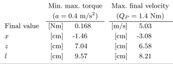
The results for both objective functions are presented in table I. Starting with x = −2 cm, z = 12 cm and l = 12 cm, the optimal values are found with respectively 1108 and 390 evaluations of both objective functions (using the Nelder-Mead Simplex method and a continuous penalty extension as discussed in Section 3.1). The global computa-tion takes less than 2 minutes with a standard PC in the Matlabr environment.
11 Which is physically irrelevant for the envisaged ejector. 12 Chosen value : 100.
Table I. optimization results of the planar ejector Min. max. torque Max. final velocity
(a = 0.4 m/s2) (Q P = 1.4 Nm) Final value [Nm] 0.168 [m/s] 5.03 x [cm] -1.46 [cm] -3.08 z [cm] 7.04 [cm] 6.58 l [cm] 9.57 [cm] 8.21
5. Application to Parallel Manipulators: Kinematic Conditioning Optimization
5.1. Dexterity of manipulators
Dexterity of a manipulator is a kinetostatic performance that can be measured from the condition number κ of its forward kinematics Jaco-bian J [18]. In other words, if this JacoJaco-bian J is defined by:
˙
x = J q˙ (25)
whereq is the joint velocity vector and˙ x the velocity vector of the end-˙ effector described by Cartesian coordinates (position and orientation), this dexterity index is the ratio of the largest singular value of J to its smallest one. This definition assumes that all entries of J have the same units. Otherwise, this dimensional inhomogeneity can be solved by introducing a normalizing characteristic length as suggested in [18]. The latter is used to divide the positioning rows of J, making it dimen-sionally homogeneous. As explained in [18], let us note that the value of the characteristic length itself comes from the minimization of the condition number over all the reachable configurations [18].
The goal is to optimize a global posture-independent performance index which is the mean of the inverses of the condition number κ over a volume V in the Cartesian space of the end-effector, also called Global Dexterity Index (GDI) [11] :
GDI = R V 1 κ dV V (26)
In the case of positioning and orientating manipulators (for instance, the Hunt platform described below), the value of κ is obviously com-puted after normalizing the Jacobian matrix, as previously explained. By analogy with the optimization proposed in [18], we suggest that the
above-mentioned characteristic length becomes an additional parame-ter of our optimization problem which initially only deals with design parameters.
5.2. Six-DoF Hunt Platform
The Hunt platform (see Figure 6) has 3 position and 3 orientation degrees of freedom which require to normalize J before computing
κ, each time the parameters change, i.e. at each call of the objective
function. As explained above, this involves an additional optimization parameter: the characteristic length LC. The nine other parameters of
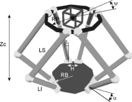
this optimization problem (see Figures 6 and [7] for more details) are the legs lengths LI,LS, the characteristic radius of the platform RP and of the base RB, the gauge H between adjoining actuators on the base, the angle α (around a vertical axis), followed by angle β (around an horizontal axis), angle ψ, and finally the vertical distance zc between the base and the center of the desired workspace volume (small cube in Figure 6).
Figure 6. Hunt platform model
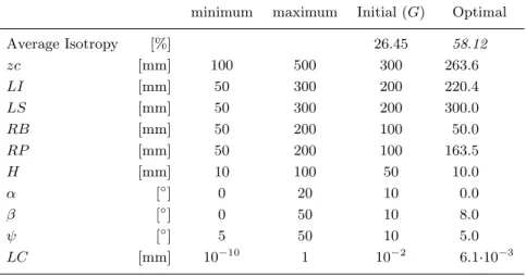
According to the research project specifications (for a surgical ap-plication), design parameters of this robot are limited by bounds (see Table II). The results obtained with the Nelder-Mead simplex method are presented in table II and initial and optimal design can be compared in Figure 7.
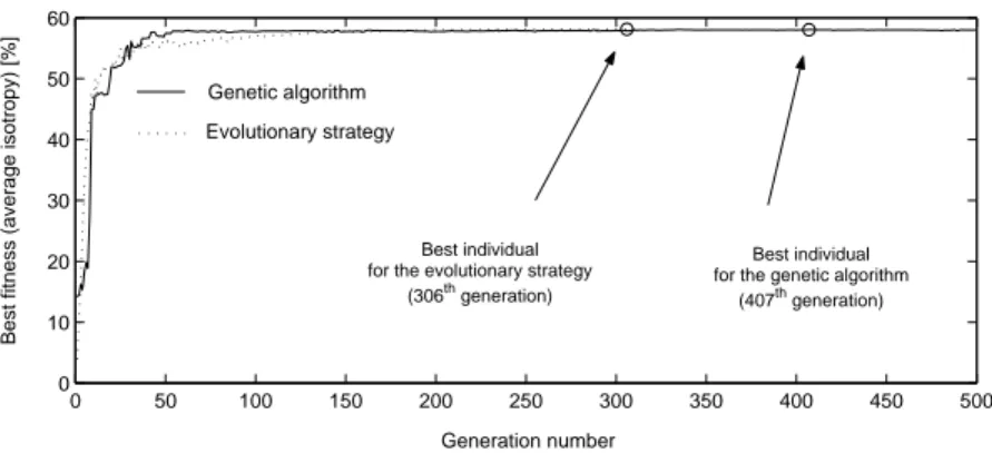
The “validation” of this result is made by using stochastic opti-mization algorithms for the same optiopti-mization problem: on the one hand, we apply a classical genetic algorithm and on the other hand, an evolutionary strategy is used.
Table II. Optimization bounds and results of the Hunt platform optimization minimum maximum Initial (G) Optimal
Average Isotropy [%] 26.45 58.12 zc [mm] 100 500 300 263.6 LI [mm] 50 300 200 220.4 LS [mm] 50 300 200 300.0 RB [mm] 50 200 100 50.0 RP [mm] 50 200 100 163.5 H [mm] 10 100 50 10.0 α [◦] 0 20 10 0.0 β [◦] 0 50 10 8.0 ψ [◦] 5 50 10 5.0 LC [mm] 10−10 1 10−2 6.1·10−3
Figure 7. Initial and optimal designs of the Hunt platform
For the genetic algorithm13, each of the 10 parameters is coded on
32 bits and the size of the population is 200. Three genetic operators are used to generate new populations. To begin, a selection is done by tournament taking – with a probability of 0.9 – the best of two individuals chosen randomly in the population. This generates half a population on which crossovers are performed, cutting chromosomes in two points. Finally, the mutation operator is applied on each bit with a fixed probability of 0.01. The evolution of the best fitness of each generation is plotted in Figure 8. The best fitness is found at the 407th generation and is equal to 58.07%.
In evolutionary strategies [3], a population of µ parents mutates in a population of λ offsprings by adding a Gaussian random variable to 13 issued from the course of Prof. V. Magnin, Ecole polytechnique universitaire de Lille, France.
0 50 100 150 200 250 300 350 400 450 500 0 10 20 30 40 50 60 Generation number
Best fitness (average isotropy) [%]
Best individual for the genetic algorithm
(407th generation) Best individual
for the evolutionary strategy (306th generation) Genetic algorithm
Evolutionary strategy
Figure 8. Optimization of the Hunt platform using stochastic methods
each optimization parameter. The standard deviation of that variable allows to control the speed of convergence [3]. It is also possible to enrich the algorithm by adding a step of recombination between parents before mutation. In our case, we choose µ = 20 and λ = 200, and also a discrete recombination as described in [3]. In Figure 8, the evolution of the best fitness of each parent generation is plotted. The best one appeared at the 306th generation and is equal to 58.12%.
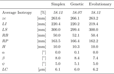
If we now compare the results of three optimization methods (Sim-plex method, genetic algorithm and evolutionary strategy), we remark that they are very similar (see Table III). The slight differences comes probably from the different convergence criteria and the choice of the various parameters involved in the optimization process (e.g.: size of populations, selection and mutation probabilities,. . . ). We may thus reasonably conclude that it should be a global optimum.
6. Conclusion and prospects
In this paper, a penalization method has been developed to optimize the design of closed-loop 3D mechanisms. The main issue lies in the as-sembling constraints and the way to solve them. So, we have shown how to exploit the conditioning of the constraints Jacobian matrix and/or the Newton-Raphson convergence to penalize the objective function. This enables to produce a nice optimization formulation that can be solved robustly, whatever the method used. Three applications are proposed: first, a simple planar ejector to illustrate the method, and then, a more 3D realistic 3D application dealing with parallel robot dexterity. Finally, a short comparison is made between optimization
Table III. Comparison between optimization methods
Simplex Genetic Evolutionary Average Isotropy [%] 58.12 58.07 58.12 zc [mm] 263.6 266.1 263.2 LI [mm] 220.4 220.2 219.4 LS [mm] 300.0 299.4 300.0 RB [mm] 50.0 52.1 50.4 RP [mm] 163.5 166.4 162.2 H [mm] 10.0 10.3 10.0 α [◦] 0.0 0.1 0.0 β [◦] 8.0 8.4 7.4 ψ [◦] 5.0 5.1 5.0 LC [µm] 6.1 6.0 6.2
results obtained with deterministic and stochastic methods, to assert the credibility of the method and of the solution.
In term of the prospects, we intend to develop further the proposed method:
• An interesting problem relates with the tuning of the
parame-ters of the objective function computation algorithm detailed in section 3.1 (i.e. the choice of point G, the type of extension. . . )
• To make the method partitioning-independent, we will try to build
a penalization criteria based on the global constraint Jacobian matrix conditioning instead of Jv (see section 3.1)
A last prospect concerns the optimization algorithm itself: other deter-ministic methods, more sophisticated than the Nelder-Mead Simplex, can be investigated and confronted.
Acknowledgements
This research has been sponsored by the Belgian Program on Interuni-versity Attraction Poles initiated by the Belgian State — Prime Minis-ter’s Office — Science Policy Programming (IUAP V/6). The scientific responsibility is assumed by its authors.
References
1. Haj-Fraj, A. and F. Pfeiffer. Optimization of Automatic Gearshifting. In Vehicle System Dynamics Supplement, 35:207–222, 2001.
2. Jiminez, J. M., G. Alvarez, J. Cardenal, and J. Cuadrado. A simple and general method for kinematic synthesis of spatial mechanisms. In Mechanism and Machine Theory, 32:323–341, 1997.
3. Datoussa¨ıd, S., O. Verlinden, and C. Conti. Application of Evolutionary Strate-gies to Optimal Design of Multibody Systems. In Multibody Systems Dynamics, 8(4):393-408, 2002.
4. Su, Y.X., B.Y. Duan, and C.H. Zheng. Genetic design of kinematically optimal fine tuning Stewart platform. In Mechatronics, 11:821–835, 2001.
5. Stocco, L.J., S.E. Salcudean, and F. Sassani. Optimal Kinematic Design of a Haptic Pen. In IEEE/ASME Transactions on Mechatronics, 6(3):210–220, 2001.
6. Fattah, A., and A.M. Hasan Ghasemi. Isotropic Design of Spatial Parallel Manipulators. In The International Journal of Robotics Research, 21(9):811– 824, 2002.
7. Ryu, J. and J. Cha. Volumetric error analysis and architecture optimization for accuracy of HexaSlide type parallel manipulators. In Mechanism and Machine Theory, 38:227-240, 2003.
8. Ceccarelli , M., and C. Lanni. A multi-objective optimum design of general 3R manipulators for prescribed workspace limits. In Mechanism and Machine Theory, 39:119-132, 2004.
9. Vallejo, J, R. Aviles, A. Hernandez, and E. Amezua. Nonlinear optimization of planar linkages for kinematic syntheses. In Mechanism and Machine Theory, 30:501–518, 1995.
10. Cabrera, J.A., A. Simon, and M. Prado. Optimal synthesis of mechanisms with genetic algorithms. In Mechanism and Machine Theory, 37:1165–1177, 2002. 11. Gallant-Boudreau, M. and R. Boudreau. An Optimal Singularity-Free Planar
Parallel Manipulator for a Prescribed Workspace Using a Genetic Algorithm. Proc. of the IDMME’2000/Forum 2000 CSME Conference, Montreal, 2000. 12. G¨ursel A., and B. Shirinzadeh. Topology optimisation and singularity analysis
of a 3-SPS parallel manipulator with a passive constraining spherical joint. In Mechanism and Machine Theory, 39:215-235, 2002.
13. Lemay, J., and L. Notash. Configuration engine for architecture planning of modular parallel robots. In Mechanism and Machine Theory, 39:101-117, 2004. 14. Datoussa¨ıd, S. Optimisatdion du comportement dynamique et cin´ematique de syst`emes multicorps `a structure cin´ematique complexe. PhD thesis, Facult´e Polytechnique de Mons, Belgium,1998.
15. Simionescu, P.A., and D. Beale. Synthesis and analysis of the five-link rear suspension system used in automobiles. In Mechanism and Machine Theory, 37:815-832, 2002.
16. N´emeth, I. A CAD tool for the preliminary design of 3-axis machine tools: syn-thesis, analysis and optimisation. PhD syn-thesis, Katholieke Universiteit Leuven, Belgium,1998.
17. Wehage, R.-A., and E.-J. Haug. Generalized coordinate partitioning for di-mension reduction in analysis of constrained dynamic systems. In Journal of Mechanical Design, 134;247–255, 1982.
18. Angeles, J. Fundamentals of Robotic Mechanical Systems: theory, methods, and algoritnms. Springer-Verlag, pp.174-190, 1997.