Checking Linear Temporal Formulas on Sequential Recursive Petri Nets
Serge HaddadLAMSADE - UPRESA 7024, Universit´e Paris IX, Dauphine Place du Mar´echal De Lattre de Tassigny, 75775 Paris cedex 16
Denis Poitrenaud
LIP6 - UMR 7606, Universit´e Paris VI, Jussieu 4, Place Jussieu, 75252 Paris cedex 05
Abstract
Recursive Petri nets (RPNs) have been introduced to model systems with dynamic structure. Whereas this model is a strict extension of Petri nets and context-free grammars (w.r.t. the language criterion), reach-ability in RPNs remains decidable. However the kind of model checking which is decidable for Petri nets be-comes undecidable for RPNs. In this work, we intro-duce a submodel of RPNs called sequential recursive Petri nets (SRPNs) and we study the model checking of the action-based linear time logic on SRPNs. We prove that it is decidable for all its variants : finite se-quences, finite maximal sese-quences, infinite sequences and divergent sequences. At the end, we analyze lan-guage aspects proving that the SRPN lanlan-guages still strictly include the union of Petri nets and context-free languages and that the family of languages of SRPNs is closed under intersection with regular languages (unlike the one of RPNs).
1. Introduction
In the area of verification theory, a great attention has been recently paid on infinite state systems. In contrast to finite state systems where theoretical and practical developments mainly focus on complexity re-duction, an essential topic in infinite state systems is to find a trade-off between expressivity of the models and decidability of verification. As the model checking of temporal logic formula is one of the most general ap-proach for verification, it has been intensively studied
in the framework of infinite-state systems.
Context-free grammars and stack automata have led to several works. In [10], it is shown that the model checking of branching time µ-calculus formula for pushdown processes is decidable. When restricting the logic to the linear time logic LTL, one obtains polyno-mial time algorithms [3].
In [2], model checking for Petri nets has been stud-ied. The branching temporal logic as well as the state-based linear temporal logic are undecidable even for restricted logics. Fortunately, the model checking for action-based linear temporal logic is decidable. The case of infinite sequences may be straightforwardly re-duced to the search of repetitive sequences studied in [11] and the case of finite sequences may be similarly reduced to the reachability problem [8]. It seems in-teresting to combine context-free grammars and Petri nets and to look for decidable properties. Indeed, for two such models - the process rewrite systems [9] and the recursive Petri nets (RPNs) [5] - the reachability problem is decidable. However, for both these two models, the model checking of action-based tempo-ral logic becomes undecidable. It remains undecid-able even for restricted models such as those presented in [1]. So for any previously existing model strictly including Petri nets and context-free grammars, the action-based linear time model checking was undecid-able.
In this work, we present a submodel of RPNs called sequential recursive Petri nets (SRPNs) and we give some decision procedures including the model check-ing. Roughly speaking, in RPNs some transitions em-ulate concurrent procedure calls by initiating a new
to-ken game in the net. The return mechanism is ensured by reachability conditions. A state of a RPN is then a tree of “token games”. In a SRPN, a procedure call freezes the current token game and the activity goes on, in the last initiated token game. A state of a SRPN is then a stack of “token games”. At first, we illustrate the increase of modelling power of SRPNs w.r.t. the Petri nets one. Indeed, a SRPN can model an infinite in-degree transition system whereas it is not the case with Petri nets (or with process algebras). Moreover, from a practical point of view the use of SRPNs often leads to a great simplification in the design process.
We then focus on the model checking problem for an action-based linear time logic. We handle the case of finite (and maximal) sequences relying on a product SRPN construction which emulates the synchronised product of a SRPN and an automaton and then reduc-ing the problem to a reachability problem (which is decidable from [5]). The case of infinite (and diver-gent) sequences is more tricky and requires to distin-guish such sequences w.r.t. the asymptotic behavior of the depth of token games. As the decision procedure is partly based on a reachability decision algorithm for Petri nets, it is not primitive recursive. Nevertheless in a modeling, the places of a SRPN are very often k-bounded with the bound k given a priori (e.g. com-puted by linear algebraic techniques). In such situa-tions, taking as inputs the SRPN and the bound, we can show that our procedure is in PSPACE. We emphasize that even in this case we deal with infinite-state sys-tems.
At last, we study the language family of SRPNs and we show that this family strictly includes the union of Petri nets and context-free languages. Moreover, unlike RPNs, this family is closed under intersection with regular languages. Finally we will discuss about complexity features and give some perspectives to this work. The complete proofs can be found in a research report [6].
2. Sequential Recursive Petri Nets 2.1. Presentation
A sequential recursive Petri net has the same struc-ture as an ordinary one except that the transitions are partitioned into two categories: elementary transitions
and abstract transitions. Moreover a starting marking is associated to each abstract transition and an effec-tively semilinear set of final markings is defined. The semantics of such a net may be informally explained as follows. In an ordinary net, a thread plays the to-ken game by firing a transition and updating the cur-rent marking (its internal state). In a SRPN there is a stack of threads (denoting the fatherhood relation) where all the threads, except the one on the top of the stack, are suspended. We call this thread, the current thread. The step of a SRPN is thus a step of the cur-rent thread. If the thread fires an elementary transition, then it updates its current marking using the ordinary firing rule. If the thread fires an abstract transition, it consumes the input tokens of the transition and creates a new thread on the top of the stack (the new current thread) which begins its token game with the starting marking of the transition. If the thread reaches a final marking, it may terminate its token game producing (in the token game of its father) the output tokens of the abstract transition which gave birth to him. In case of a single thread in the stack, one obtains an empty stack.
Definition 2.1 (Sequential Recursive Petri nets) A sequential recursive Petri net is defined by a tuple N = hP, T, W−, W+, Ω, Υi where
• P is a finite set of places, T is a finite set of tran-sitions.
• A transition of T can be either elementary or ab-stract. The sets of elementary and abstract tran-sitions are respectively denoted by Tel and Tab
(with T = Tel] Tabwhere ] denotes the disjoint
union).
• W−and W+are the pre and post flow functions defined from P × T to IN.
• Ω is a labeling function which associates to each abstract transition an ordinary marking (i.e. an element of INP) called the starting marking of t. • Υ is an effective representation of semilinear set
of final markings.
A semilinear set of markings is a finite union of linear sets of markings. A linear set L is defined
by a marking m0 and a finite family of markings {m1, . . . , mk} such that L = {m | ∃λ1, . . . , λk ∈
INk, m = m0+Pi=1,...,kλi.mi}. An effective rep-resentation is any reprep-resentation which can be reduced (by an algorithm) to this standard representation. For instance, any system of linear (in)equations on the places marking is an effective representation.
Definition 2.2 (Extended marking) An extended marking tr of a sequential recursive Petri net N = hP, T, W−, W+, Ω, Υi is a labeled list tr = hV, M, E, Ai where
• V is the set of nodes. If V is not empty then V contains a bottom node vB and a top node vT.
These nodes are identical iff |V | = 1. • M is a mapping V → INP,
• E ⊆ (V \ {vT}) × (V \ {vB}) is the set of edges with:
∀v ∈ V \ {vB} there is only one node called pred(v) such that (pred(v), v) ∈ E
∀v ∈ V \ {vT} there is only one node called succ(v) such that (v, succ(v)) ∈ E
• A is a mapping E → Tab.
A marked sequential recursive Petri net hN, tr0i is
a sequential recursive Petri net N associated to an initial extended marking tr0. For sake of simplicity
(w.l.o.g.), we will require that there is only one node in any initial extending marking.
When we will deal with different extended ings, we will denote the items of an extending mark-ing tr as a function of the extendmark-ing markmark-ing (e.g. vB(tr)). The empty list is denoted by ⊥. Any ordi-nary marking m can be seen as an extended marking, denoted by dme, consisting of a single node. An el-ementary step of a SRPN may be either a firing of a transition or an ending of a token game (called a cut step and denoted by τ ).
Definition 2.3 A transition t is enabled in an ex-tended marking tr 6=⊥ (denoted by tr−→) if ∀p ∈t P, M (vT)(p) ≥ W−(p, t) and a cut step is enabled
(denoted by tr−→) if M (vτ T) ∈ Υ
Definition 2.4 The firing of an enabled elementary step t from an extended marking tr = hV, M, E, Ai leads to the extended marking tr0 = hV0, M0, E0, A0i (denoted by tr−→trt 0) depending on the type of t.
• t ∈ Tel
– V0 = V , E0 = E , ∀e ∈ E, A0(e) = A(e), ∀v0∈ V \ {v T}, M0(v0) = M (v0) – ∀p ∈ P, M0(vT)(p) = M (vT)(p) − W−(p, t) + W+(p, t) • t ∈ Tab – V0 = V ∪ {v0} , E0 = E ∪ {(vT, v0)}, ∀e ∈ E, A0(e) = A(e) , A0((v T, v0)) = t – ∀v00∈ V \ {vT}, M0(v00) = M (v00), – ∀p ∈ P, M0(vT)(p) = M (vT)(p) − W−(p, t) – M0(v0) = Ω(t)
where v0 is a fresh identifier absent in V ; v0 = vT(tr0).
• t = τ
– V0 = V \ {vT} , E0 = E ∩ (V0 × V0) , ∀e ∈ E0, A0(e) = A(e)
– ∀v0∈ V0\ {pred(vT)}, M0(v0) = M (v0) – ∀p ∈ P, M0(pred(v T))(p) = M (pred(vT))(p) + W+(p, A(pred(v T), v))
Let us notice that if |V | = 1 then the firing of τ leads to to empty list ⊥.
The depth of an extended marking is defined as |V |. For an extended marking tr, its depth is denoted by depth(tr). A firing sequence is defined as usual: a sequence σ = tr0.t0.tr1.t1. . . . .tn−1.trn is a fir-ing sequence (denoted by tr0−→trσ n) iff tri−→trti i+1 for i ∈ [0, n − 1]. We define the depth of σ as the maximal depth of tr1, tr2, . . . , trn. In the se-quel, for sake of simplicity, σ will be often denoted by σ = t0.t1. . . . .tn−1
2.2. An illustrating example
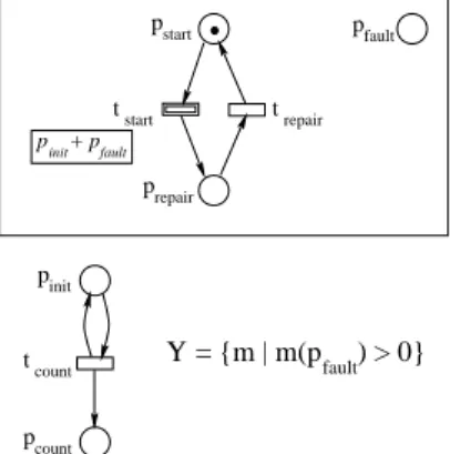
In order to analyze fault-tolerant systems, the engi-neer starts from a nominal system and then introduces the faulting behavior as well as the repairing mecha-nisms. We limit ourselves to an elementary system. The nominal system periodically records some mea-sure of the environment (elementary transition tcount).
The number of measures is stored in place pcount. The complete system is obtained by adding the bordered part of the figure 1. The behavior of the SRPN can be described as follows. Initially and in the crash state, the extended marking consists in a single node. A to-ken in the place prepair indicates that one is repairing the system while a token in pstart indicates that the system is ready. When the abstract transition tstart is fired the correct behavior is “played” by the new thread. If this thread dies by a cut step, a crash state is reached. As the place pf ault is always marked in the correct system and from the very definition of Υ, the occurrence of a fault is always possible. With addi-tional places and modifying Υ, we could model more complex fault occurrences (e.g. conditioned by soft-ware execution). p + p p p p t t Υ= {m | m(p ) > 0}fault p t p count count start start repair repair fault init fault init
Figure 1. a basic fault-tolerant system
The SRPN switches between states with a single node and states with a bottom and a top node. How-ever, the number of reachable markings in the top node is infinite (the place pcount is unbounded). In other words, the crash state can be reached from an infi-nite number of states which means that the transition system associated to a SRPN may have some nodes with an infinite in-degree. This capability is neither shared by Petri nets nor by process algebras. Con-sequently, such models cannot represent this kind of systems. More generally, any transition system where some node has an infinite in-degree can neither be modelled by Petri nets nor by process algebras. We emphasize that even in the case of finite state transi-tion systems such modelisatransi-tions are rather difficult and lead to very intricate Petri nets (or process algebras) whereas the same design is quite easy with SRPNs.
In [7], the model of recursive Petri nets is illustrated by additional examples and compared to other similar models.
3. Model Checking
The model checking that we investigate applies on action based linear-time formulas represented by B¨uchi automaton. The usual verification method con-sists to check the existence of a sequence of the sys-tem fulfilling the negation of the formula. Depending on the kind of the sequence, different semantics have been defined. We will study the main ones: finite se-quences, maximal finite sequences (leading to a dead-lock), infinite sequences, divergent sequences (infinite sequences ended by a non observable subsequence). Definition 3.1 (B ¨uchi automaton) A B¨uchi automa-ton is a tuple A = hΣ, Q, ∆, q0, F i where Σ is an
alphabet, Q a finite set of states, ∆ ⊆ Q × Σ × Q a transition relation, q0∈ Q an initial state and F ⊆ Q
a set of accepting states.
As usual, we denote by q−→qa 0 that (q, a, q0) ∈ ∆. Moreover, the extension of−→ to words over Σ is de-noted by=⇒ and is defined as follows:
• ∀q ∈ Q, q=⇒qλ
• ∀q, q0 ∈ Q, q=⇒qωa 0⇔ ∃q00, q=⇒qω 00∧ q00 a−→q0
A run r of A on a finite word ω = a1. . . an over
Σ is a finite sequence q0, . . . , qn on Q such that ∀j ∈
[1, n], qj−1 aj
−→qj. A run r of A on a infinite word ω = a1. . . ai. . . is an infinite sequence q0, . . . , qi, . . . on Q such that ∀j > 0, qj−1−→qaj j. We now define how such an automaton recognizes and accepts finite and infinite words.
Definition 3.2 (Recognition and acceptance) Let A = hΣ, Q, ∆, q0, F i be a B¨uchi automaton.
• Let ω be a finite word over Σ. Then ω is recog-nized by A if there is a run on ω. Moreover, if one of these runs is ended by a state of F then ω is accepted by A. L(A) denotes the set of finite words accepted by A.
• Let ω = a1. . . ai. . . be an infinite word over Σ.
Then ω is recognized by A if there is a run r = q1, . . . qi, . . . on ω. Moreover, if one of these runs
fulfills |{k | qk∈ F }| = ∞ then ω is accepted
by A. L∞(A) denotes the set of infinite words accepted by A.
The observable behaviors of the SRPN we will con-sider are defined via a labeling function. A labeled marked sequential recursive Petri net is a marked SRPN and a labeling function h defined from the tran-sition set T ∪ {τ } to an alphabet Σ plus λ (the empty word). As usual, h is extended to sequences.
Before the study of the model checking problem, we introduce A SRPN representing the synchronised product of a given SRPN and an automaton both la-beled on a same alphabet. The product SRPN is con-structed from the places of the original one by adding a place set Q which corresponds to the states of the automaton. As usual, the elementary transitions are synchronized with the ones of the automaton using these new places. For each extended arc q=⇒qa 0 (with a ∈ Σ ∪ {λ}) of the automaton and for each elemen-tary transition t such that h(t) = a, an elemenelemen-tary transition t.q.q0, having W−(t) + q as pre-condition and W+(t) + q0 as post-condition, is added. When an abstract transition is fired a new node appears and, due to the SRPN definition, the token game is lim-ited to this node. Then, we have to predict the state reached by the automaton when the new token game will be ended. The abstract transitions constructed in the product SRPN are denoted t.q.q0.q00where the pre-fix t.q.q0expresses the same conditions as for the ele-mentary transitions (excepted that t is an abstract tran-sition of the original net). For each state q00 ∈ Q such an abstract transition is added (the prediction is non deterministic). To ensure that the predicted state is ef-fectively reached when the cut step closing the token game is fired, a set of places Q (complementary to Q) is used. The firing of an abstract transition t.q.q0.q00 leads to the creation of a new node for which its start-ing markstart-ing has the place q00 marked. Using these places, the effectively semilinear set of final markings is built in order to ensure that the predicted state is ef-fectively reached. Let us notice that this composition corresponds to a weak synchronization as some transi-tions of the SRPN can be labeled by λ.
Definition 3.3 (Product SRPN) Let A =
hΣ, Q, ∆, q0i be an automaton and S = hhN, dm0ei, Σ, hi a labeled SRPN. The product
SRPN of A and S is a labeled marked SRPN hhN0, dm0 0ei, Σ, h0i defined by • P0 = P ∪ Q ∪ Q, m0 0 = m0+ q0 • T0 el= {t.q.q0 | (t ∈ Tel)∧(q, q0 ∈ Q)∧(q h(t) =⇒q0)} • ∀t.q.q0 ∈ T0 el, – h0(t.q.q0) = h(t), – W0−(t.q.q0) = W−(t) + q, W0+ (t.q.q0) = W+(t) + q0 • T0 ab = {t.q.q0.q00 | (t ∈ Tab) ∧ (q, q0, q00 ∈ Q) ∧ (q=⇒qh(t) 0)} • ∀t.q.q0.q00∈ Tab0 , – h0(t.q.q0.q00) = h(t) – W0−(t.q.q0.q00) = W−(t) + q, W0+(t.q.q0.q00) = W+(t) + q00 – Ω0(t.q.q0.q00) = Ω(t) + q0+ q00 • Υ0 = {m + q + q0 | (m ∈ Υ) ∧ (q, q0 ∈ Q) ∧ (q=⇒qh(τ ) 0)} • h0(τ ) = h(τ )
The next proposition shows the soundness of the product SRPN construction. This SRPN simulates the synchronized product of the orginal net with the B¨uchi automaton w.r.t. the language criterion.
We denote by L(N, tr0, T rf) (where T rf is a fi-nite set of extended markings) the set of firing se-quences (mapped on (T ∪ τ )∗) of N from tr0 to an extended marking of T rf. This set is called the lan-guage of N . The lanlan-guage of a labeled marked SRPN hhN, tr0i, Σ, hi for a finite extended marking set T rf is defined by h(L(N, tr0, T rf)) where h is extended to languages.
For sake of simplicity, we impose that the sets of ter-minal states are composed by extended marking lim-ited to a single node. One can remark that this condi-tion is not a theoretical restriccondi-tion.
Proposition 3.4 (SRPN product property) Let A = hΣ, Q, δ, q0, F i be a B¨uchi automaton, S = hhN, dm0ei, Σ, hi a labeled SRPN and Mfa set of ter-minal markings. Let hhN0, dm0
0ei, Σ, h0i be the
prod-uct SRPN of hΣ, Q, δ, q0i and S and Mf0 = {dm + qe | dme ∈ Mf ∧ q ∈ F }. The following equality holds h0(L(N0, dm00e, Mf0)) = h(L(N, dm0e, Mf)) ∩ L(A)
Sketch of proof:
The main part of the proof follows from the construc-tion presented below. The critical point is that al-though the product SRPN allows “bad” sequences (i.e. not recognized by the automaton), such ones cannot lead to a terminal extended marking of the product
SRPN. ♦
We now adapt the product construction to reduce the model-checking problem of finite sequences to a reachability problem for the product SRPN which is known to be decidable [5].
Theorem 3.5 (Acceptance of finite sequences) Let A = hΣ, Q, δ, q0, F i be a B¨uchi automaton and S = hhN, dm0ei, Σ, hi a labeled SRPN. The existence of a finite firing sequence σ of S such that h(σ) is accepted by A is decidable.
Sketch of proof:
Let hhN0, dm00ei, Σ, h0i be the product SRPN of A and S. We construct a new SRPN hN00, dm00 0ei in the fol-lowing way: • N00 = N0 except for Υ00 = Υ0 ∪ {m | ∃q ∈ F, m ≥ q} • m00 = m000
It can be shown that the existence of a finite fir-ing sequence σ of S such that h(σ) is accepted by A is equivalent to the reachability of ⊥ by hN00, dm000ei. The critical point is that considering sequences of N00 reaching ⊥, then the shortest ones correspond to se-quences σ of the original net such that h(σ) is accepted
by A. ♦
Maximal finite sequences are handled similarly with a more complex construction. In this new prod-uct, a pair of places is added to allow the prediction of deadlocks when creating a new node in the stack and the semi-linear set of terminal markings is adapted to detect deadlocks.
Theorem 3.6 (Acceptance of maximal sequences) Let A = hΣ, Q, δ, q0, F i be a B¨uchi automaton and S = hhN, dm0ei, Σ, hi a labeled SRPN. The existence
of a finite firing sequence σ of S such that σ leads to a deadlock of N and h(σ) is accepted by A is decidable.
For the infinite case, the technique based on the SRPN product is not sufficient to obtain a decision procedure. We have developed an original proof tech-nique based on the analysis of the sequences depend-ing on the asymptotic behavior of the depth of the vis-ited extended markings.
We are looking for an infinite firing sequence of the SRPN accepted by a B¨uchi automaton. We will per-form two independent searches depending on a char-acteristic of the sequence: the asymptotic behavior of the depth of the sequence.
Let σ = dm0e−→trt1 1−→ . . . trt2 i−1−→trti i. . . be an infinite sequence, we define dinf (σ) = lim infi→∞depth(tri) (defined by limi→∞infj≥i{depth(trj)}). dinf (σ) always exists but it can be either finite or infinite.
In case of a finite value, there exists a strictly in-creasing sequence of indexes i1, . . . , ik, . . . such that:
• beyond i1 the set of indexes {i1, i2, . . . , ik, . . .} is exactly the indexes for which the depth of the visited extended markings is equal to dinf (σ) (∀i ≥ i1, depth(tri) = dinf (σ) ⇔
i ∈ {i1, i2, . . . , ik, . . .})
• beyond i1the depth of the visited extended mark-ings will be greater or equal than dinf (σ) (∀i ≥ i1, depth(tri) ≥ dinf (σ))
• i1 is the first index from which the depth of the visited extended markings will be no more less than dinf (σ)
(∀i < i1, ∃j ≥ i, depth(trj) < dinf (σ))
So σ will be decomposed as dm0e−→trσ0 i1 σ1 −→ . . . trik σk −→trik+1. . . where σ0
ends with the firing of an abstract transition leading to an extended marking of depth dinf (σ) (with the creation of a new node) and σk is either a firing of an elementary transition in this node or a sequence beginning by the firing of an abstract transition in this node and ended by a corresponding cut step.
In case of an infinite value, there exists a strictly in-creasing sequence of indexes i1, . . . , ik, . . . such that:
• k is the depth of the extended marking trik
• beyond ikthe depth of the visited extended mark-ings will be greater or equal than k
(∀i ≥ ik, depth(tri) ≥ k)
• ikis the first index from which the depth of vis-ited extended markings will be no more less than k
(∀i < ik, ∃j ≥ i, depth(trj) < k) So σ will be decomposed as: dm0e = tri1 σ1 −→tri2 σ2 −→ . . . trik σk −→trik+1. . . where
σkbegins by a firing in an extended marking of depth k, ends with the firing of an abstract transition leading to an extended marking of depth k + 1 and such that all the extended markings visited by σk have a depth greater or equal than k.
So the first step of the proof consists in developping a procedure to check the existence of some finite firing subsequences beginning and ending in the same node of two extended markings and corresponding to paths of the B¨uchi automaton. Indeed, we need another pro-cedure which restricts the sequences to those which visit an accepting state of the automaton. In either case, these procedures are very similar to the model checking for finite sequences.
We are now in position to explain the two main pro-cedures. Looking for a sequence σ with dinf (σ) fi-nite, we first compute the couples of starting markings and automaton states reachable by a firing sequence. We build an ordinary Petri net representing an abstract view of sequences of the SRPN (recognized by the au-tomaton) where the successive extended markings vis-ited by the sequence are infinitely often reduced to a single node. Then, for each couple as initial marking of this Petri net, we look for an infinite sequence visit-ing a subset of transitions infinitely often (this can be done by the algorithm of [11]).
Looking for a sequence σ with dinf (σ) infinite, we build a graph where the nodes are the computed cou-ples of the first procedure and an edge denotes that one node has been reached from the other one by a sequence increasing by one the depth of the visited ex-tended markings and such that the intermediate sub-sequences never decrease the depth below its initial value. The edges are partitioned depending on the visit by the sequence of an accepting state of the B¨uchi au-tomaton. Then the existence of an accepting infinite sequence is equivalent to the existence of some kind
of strongly connected component.
Theorem 3.7 (Acceptance of infinite sequences) Let A = hΣ, Q, δ, q0, F i be a B¨uchi automaton and S = hhN, dm0ei, Σ, hi a labeled SRPN. The existence of an infinite sequence σ of hN, dm0ei such that h(σ)
is an infinite word accepted by A is decidable. Divergent sequences are handled similarly. Theorem 3.8 (Acceptance of divergent sequences) Let A = hΣ, Q, δ, q0, F i be a B¨uchi automaton and S = hhN, dm0ei, Σ, hi a labeled SRPN. The existence
of an infinite sequence σ of hN, dm0ei such that h(σ)
is a finite word accepted by A is decidable.
All our decision procedures use the decidability of reachability in RPNs (based on reachability in Petri nets). Thus none of them are primitive recursive. However it must be emphasized that very often un-bounded Petri nets correspond to systems with dy-namic structure. Modelling such systems with SRPNs leads to infinite states SRPNs with bounded places. Moreover the bound may be computed by structural analysis. In such cases, complexity of our decision procedure is reduced as stated by the next theorem. Theorem 3.9 (Complexity of model-checking) Let A = hΣ, Q, δ, q0, F i be a B¨uchi automaton and S = hhN, dm0ei, Σ, hi a labeled k-bounded SRPN.
The problem of existence of a finite (maximal finite, infinite, divergent) sequence σ of hN, dm0ei such that h(σ) is a word accepted by A is PSPACE-complete w.r.t. the size of A and S.
4. Language Properties
In order to discuss about expressivity of models, different criteria may be applied such like generated languages, behavioural equivalences,. . . In this sec-tion, we focus on the properties of the languages gen-erated by SRPNs and we compare it with the standard hierarchy of languages.
Theorem 4.1 (SRPN closure) The family of SRPN languages is closed under intersection with regular languages.
Sketch of proof:
Follows straightforwardly from proposition 3.4 ♦ Theorem 4.2 (Strict inclusion) SRPN languages strictly include the union of context-free and Petri net languages
Proof:
It is obvious that any PN is a SRPN. Moreover, in [5], it is demonstrated that any context-free language can be simulated by a RPN. We can remark that the proposed construction of the RPN corresponding to a context-free language leads to a SRPN (i.e. the initial extended marking is limited to a single node and all the reachable states are stacks and only the top node is active). In the same paper, it is shown that RPN languages strictly include the union of context-free and Petri net languages. The proof of this result ex-hibits a RPN for which its language is neither PN nor context-free language. We can remark that this RPN behaves as a SRPN. Then, we can conclude that the language family of SRPN strictly includes the union of the context-free and PN languages. ♦ Moreover, in [4], it is demonstrated that the RPN languages are not closed under intersection with regu-lar ones. Then the theorem 4.1 leads to the next one. Corollary 4.3 (SRPN versus RPN) The family of SRPN languages is strictly included in the family of RPN languages.
5. Conclusion
In this work, we have introduced sequential recur-sive Petri nets and studied their theoretical features. From a modeling point of view, an important charac-teristic of SRPNs is their capability to generate infi-nite in-degree transition systems. Such a feature makes possible to model dynamic systems which can be han-dled neither by process algebra nor by Petri nets.
In the second part of the paper, we have focused on the model checking for an action-based linear time logic and obtained different decision procedures de-pending on the semantics of the logic. These proce-dures are not primitive recursive in the general case but restricting the SRPNs to bounded ones (with an a priori known bound), the model checking problem is shown to be PSPACE-complete.
At last, we have studied the language family of SRPNs and proved that this family strictly includes the union of Petri nets and context-free languages. More-over, unlike RPNs, this family is closed under inter-section with regular languages.
We now plan to study how we can extend SRPNs preserving the model checking decidability.
References
[1] A. Bouajjani and P. Habermehl. Constraint properties, semi-linear systems, and Petri nets. In Proc. of CON-CUR’96, volume 1119 of Lecture Notes in Computer Science. Springer Verlag, 1996.
[2] J. Esparza. Decidability of model checking for infinite-state concurrent systems. Acta Informatica, 34:85–107, 1997.
[3] A. Finkel, B. Willems, and P. Wolper. A direct sym-bolic approach to model checking pushdown systems. In Proc. of INFINITY’97, 1997.
[4] S. Haddad and D. Poitrenaud. Decidability and un-decidability results for recursive Petri nets. Technical Report 019, LIP6, Paris VI University, Paris, France, Sept. 1999.
[5] S. Haddad and D. Poitrenaud. Theoretical aspects of recursive Petri nets. In Proc. 20th Int. Conf. on Ap-plications and Theory of Petri nets, volume 1639 of Lecture Notes in Computer Science, pages 228–247, Williamsburg, VA, USA, June 1999. Springer Verlag. [6] S. Haddad and D. Poitrenaud. A model check-ing decision procedure for sequential recur-sive petri nets. Technical Report 024, LIP6, Paris VI University, Paris, France, Sept. 2000. http://www.lip6.fr/reports/lip6.2000.024.html. [7] S. Haddad and D. Poitrenaud. Modelling and
analyz-ing systems with recursive Petri nets. In Proc. of the Workshop on Discrete Event Systems - Analysis and Control, pages 449–458, Gand, Belgique, Aug. 2000. Kluwer Academics Publishers.
[8] E. Mayr. An algorithm for the general Petri net reach-ability problem. In Proc. 13th Annual Symposium on Theory of Computing, pages 238–246, 1981.
[9] R. Mayr. Decidability and Complexity of Model Checking Problems for Infinite-State Systems. PhD thesis, TU-M¨unchen, 1997.
[10] I. Walukiewicz. Pushdown processes: Games and model checking. In Int. Conf. on Computer Aided Ver-ification, volume 1102 of Lecture Notes in Computer Science, pages 62–74. Springer Verlag, 1996. [11] H.-C. Yen. A unified approach for deciding the
exis-tence of certain Petri net paths. Information and Com-putation, 96:119–137, 1992.