Learning and memory within chaotic neurons

LEARNING AND MEMORY WITHIN CHAOTIC NEURONS

THE SIS SUBMITTED

IN PARTIAL FULFILLMENT OF THE REQUIREMENTS FOR THE DEGREE OF

DOCTOR OF PHILOSOPHY IN COGNITIVE COMPUTING

BY

MARIOAOUN

APPRENTISSAGE ET MÉMOIRE AU SEIN DES NEURONES CHAOTIQUES

THÈSE PRÉSENTÉE

COMME EXIGENCE PARTIELLE

DU DOCTORAT EN INFORMATIQUE COGNITIVE

PAR

MARIOAOUN

Avertissement

La diffusion de cette thèse se fait dans le respect des droits de son auteur, qui a signé le formulaire Autorisation de reproduire et de diffuser un travail de recherche de cycles supérieurs (SDU-522 - Rév.07 -2011 ). Cette autorisation stipule que «conformément à l'article 11 du Règlement no 8 des études de cycles supérieurs, [l'auteur] concède à l'Université du Québec à Montréal une licence non exclusive d'utilisation et de publication de la totalité ou d'une partie importante de [son] travail de recherche pour des fins pédagogiques et non commerciales. Plus précisément, [l'auteur] autorise l'Université du Québec à Montréal à reproduire, diffuser, prêter, distribuer ou vendre des copies de [son] travail de recherche à des fins non commerciales sur quelque support que ce soit, y compris l'Internet. Cette licence et cette autorisation n'entraînent pas une renonciation de [la] part [de l'auteur] à [ses] droits moraux ni à [ses] droits de propriété intellectuelle. Sauf entente contraire, [l'auteur] conserve la liberté de diffuser et de commerciali$er ou non ce travail dont [il] possède un exemplaire.»

First of ali, I am grateful to God for paving me the way in the pursuit of my goals, for driving my life and giving tne the faith to overcome ali obstacles. I atn grateful to my country Canada for giving me the opportunity to express my best self by providing me stability, security and peace of mind. Also, I am grateful to my delightful university, its friendly people and amazing excellent personnel. I can 't miss to acknowledge the backing of Mr. Sylvain Le May, head of the Handicap Students Service in our university.

On the academie leve!, I would like to thank Dr. Mounir Boukadoum, for embracing me initially, for his hypothesis towards modeling the human 1nemory that matched tny hypothesis, and upon which we started the joumey of my Phd Thesis. From our first meeting together, I sensed his opened tnindset and his strong indefinable courage. Being my director I thank him for continually believing in my potential and for his supervision ail these years. As well, I thank Dr. Sylvain Chartier and Dr. Jean Philippe Thivierge for their co-direction, our department and its head: Dr. Lounis Hakim.

On the research leve!, I would like to offer a special thank to Prof. Nigel T. Crook from Oxford Brooks University, for his ingenuity, his original research and his insights that irrigated the bloom of my research (starting fr01n the year 2006) and made it flourish ali the years afterward. l'rn honored to mention my sincere respect to Oxford Brooks University for their affluent accommodation, while I was presenting my early research at their premises upon the invitation I received from Prof. Crook. That experience opened my eyes and my mind wide large in the field of chaotic neural computing and gave me the ultimate strength that I required to proceed forward.

On a persona] leve!, I thank Chantal K., Mitri D. and Amine S. whom without their invaluable and unconditional continuous support 1 could neither resist nor endure my persistent physical and moral difficulties. Without them 1 couldn't do this thesis ...

This thesis is dedicated to my father who called me an engineer when 1 was just seven years old, who was fascinated by perpetuai motion and took the opportunity to demonstrate it to me, my fa th er who observed th at same specie of flow ers have exact number of petais, thus,

ACKNOWLEGMENTS ... iii

DEDICATION ... iv

TABLE OF CONTENTS ... v

LIST OF TABLES ... viii

LIST OF FIGURES ... ix

LIST OF ABBREVIATIONS ... xii

ABSTRACT ... _. ... xiv

RÉSUMÉ ... xvi

IN"TRODUCTION ... 1

CHAPTER 1 Fundamentals, background and thesis initiation ... 4

1.1 Scope: Cognitive informatics and its current paradigms ... 4

1.2 Formai definition of a dynmnical system ... 6

1.3 Neural computing and neuron models ... 8

1.3.1 The biological neuron ... 8

1.3.2 Basic neuron models ... 9

1.3 .3 Threshold gates: McCulloch and pitts neuron model ... 10

1.3.4 Sigmoidal gates: Analogue output. ... 11

1.3.5 Spiking neuron model ... 13

1.4 General description of the thesis problem and guidance to follow ... 16

1.5 Chaos theory and the nonlinear dynamic state neuron ... 18

1.7 Thesis statement, objectives and thesis organization ... 29

CHAPTER 2 lnvestigating synaptic plasticity with chaotic spiking neurons and regular spiking neurons ... 30

2.1 Introduction ... 30

2.2 Neural network architecture ... 32

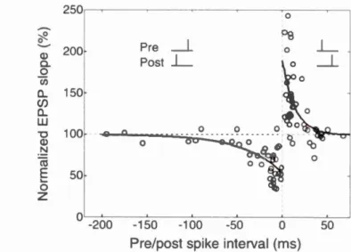
2.3 Synaptic plasticity based on spike ti me dependent plasticity (STDP) ... 36

2.4 STDP win dow ... 38

2.5 Implementing STDP in RNN of spiking neurons with ti me delay ... 40

2.6 Behavior of the RNN using STDP ... 42

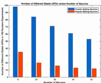
2.7 Unstable periodic orbits (UPOs) in RNN using STDP ... 47

2.8 Conclusion ... 49

2.9 Concluding remarks ... 49

CHAPTER 3 Theory of neuronal groups based on chao tic sensitivity ... 52

3.1 Introduction ... 52

3.2 The leaky integrate and fire neuron ... 55

3.3 The adaptive exponential integrate and fire (AdEx) neuron ... 56

3.4 Controlling the chaotic behavior of the AdEx neuron ... 58

3.5 The resonate and fire neuron ... 63

3.6 The neural network architecture ... 65

3. 7 Visualizing RAF neuronal groups ... 70

3.8 Separation property of neuronal groups ... 76

3.9 Large number ofRAF neuronal groups ... 87

3.10 Discussion ... 93

3.11 Conclusion ... 97

CHAPTER 4 Data classification and learning based on fi ring rates of chaotic spiking neurons and differentiai evolution ... 100

4.1 Introduction ... 100

4.3 Relationship between fi ring rates and number of neurons ... Ill

4.4 Data classification based on firing rates of chaotic spiking neurons ... 118

4.5 Experimental results ... 121

4.6 Discussion ... 129

4.7 Conclusion ... 131

CONCLUSION ... 133

Advantages, Disadvantages, Potentials and Limitations ... 133

Fin al Remarks ... 13 7 ANNEXE I ... 139 ANNEXE II ... 154 ANNEXE III ... 163 ANNEXE IV ... 168 APPENDIX A ... 169 BIBLIOGRAPHY ... 188

TABLE

2.1 Configuration of the AdE x neuron parameters ... 34

3.1 Parameters configuration of the AdE x neuron in two modes ... 57

3.2 Results of experiments where input current is varied ... 72

3.3 Spikes occurrences of different values of the adaptation reset parameter ... 82

3.4 Experiments protocol by varying the time delay and the ti me of first spike ... 87

3.5 Results of the experiments ... 89

4.1 Parameters configuration of the AdEx neuron in chaotic mode ... 104

4.2 Results of9 experiments by varying the number ofneurons ... 112

4.3 Neural network settings ... 122

4.4 DEA settings for the IRIS dataset. ... 124

4.5 Average firing rates and average number ofneurons ... 124

4.6 DEA settings for the breast cancer dataset ... 126

4.7 Average firing rates and average number ofneurons ... 127

FIGURE

1.1 Typical Sketch of a biological neuron ... 9

1.2 The McCulloch and Pitts neurons model. ... 10

1.3 The sigmoid activation function ... 12

1.4 Illustration of a spike ... 14

1.5 Spike neuron model ... .-... 15

1.6 The chaotic attractor ofRossler ... 22

1. 7 The NDS neuron voltage ... 24

1. 8 The phase space diagram ... 25

1.9 Chaos control ... 26

1.10 Phase space diagram ofEEG bulb ... 27

2.1 Neural network architecture ... 33

2.2 Curve plot of the STDP protocol ... 39

2.3 STDP time window from e1npirical data ... 40

2.4 Neural network spikes output ... 43

2.5 Periodic spikes synchronization ... 44

2.6 Proof of synchronization of neurons output spikes ... 45

2. 7 Proof of synchronization of neurons voltages ... 45

2.8 Proof of synchronization ofneurons adaptation variables ... 46

2.9 Average weight of the connections inside the RNN ... 46

2.10 STDP win dow of the RNN ... 4 7 2.11 Comparison of the number of different stabilized UPOs ... 48

3.1 Plot of the activity ofLIF Neuron ... 56

3.2 Plot of the regular activity of AdEx neuron ... 58

3.4 Chaos control- Activity of AdEx neuron ... 60

3.5 Chaos control- Evolution of Adaptation variable of AdEx neuron ... 61

3.6 Chaos control- Synchronization ofneuron variables ... 62

3.7 Phase space plot of the AdEx Neuron after chaos control.. ... 62

3.8 Voltage activity and firing of the RAF neuron ... 65

3.9 Neural Network architecture ... 66

3.10 Network architecture with a variable input current ... 71

3.11 Visualization of 9 neuronal groups ofRAF neurons ... 76

3.12 Separation of single spike input patterns ... 79

3.13 Behavior of AdEx neurons for different values ofreset parameters ... 80

3.14 Amelioration of the separation of single spike input patterns ... 81

3.15 Further amelioration of the separation of single spike input patterns ... 83

3.16 Separation of single spike input patterns ... 84

3.17 Separation of single spike input patterns ... 84

3.18 Additional example of the separation of single spike input patterns ... 85

3.19 Separation of multiple spikes input patterns ... 86

3.20 Plot of the minimum and maxünum number ofactivated RAF neurons ... 90

3.21 Plot of the RAF neuronal groups per ti me delay ... 91

3.22 Plot of the total number of unique RAF neuronal groups ... 92

3.23 Polynomial regression of the total number ofRAF neuronal groups ... 93

3.24 Exatnple ofpolychronous groups ... 94

3.25 Bursting activity simulated using chaos control ... 97

4.1 Neural network architecture ... 103

4.2 Neural network spike output. ... 107

4.3 Periodic spikes synchronization ... 108

4.4 Proof of synchronization of output spikes of ail neurons ... 109

4.5 Pro of of synchronization of voltages of ali neurons ... 109

4.6 Pro of of synchronization of adaptation variables of ali neurons ... 110 4. 7 Histogram of inter-spike intervals ... Ill

4.8 Firing rate vs. number of neurons ... 113

4.9 Firing rate vs. number of neurons- random isolation ti me ... 114

4.10 Fi ring rate vs. number of neurons- rand01n connection 's ti me delay ... 115

4.11 Fi ring rate vs. ti me delay ... 116

4.12 Firing rate vs. ti me delay and number of neurons ... 117

4.13 IRIS testing data samples class distribution ... 125

4.14 10 fold cross validation performed on IRIS dataset ... 126

4.15 Breast cancer testing data samples class distribution ... 127

ACM- Association for computing machinery AdEx -Adaptive exponential integrate and fire AFR - Average firing rate

ANN- Average number ofneurons AP- Approximation property

ASAP- Adjustable separation and approximation properties CC- Chaos control

CI- Cognitive informatics

CN- Computational neuroscience DE- Differentiai evolution

DEA - Differentiai evolution algorithm

DEFR- Differentiai evolution using firing rates EEG- Electro encephalogram

EPSP- Excitatory postsynaptic potential FR - F iring rate

FRC - Frequency response curve ISis- Inter spike intervals LIF - Leaky integrate and fire LTD- Long-term depression LTP- Long-term potentiation MCP- McCulloch and pitts

MIT- Massachusetts institute of technology ML- Machine learning

MLP- Multilayer perceptron MLP- Multilayer perceptrons

NRS- Neurosciences research foundation NTC- Nonlinear transient computation

NTCM - Nonlinear transient computing machine ODE- Ordinary differentiai equation

PAC- Probably approximately correct RAF - Resonate and fire

RC - Reservoir computing RNN- Recurrent neural network

SDFR- Standard deviation of fi ring rates SFC- Spike feedback control

SP- Separation property

SRC- Sizable reservoir computing SRM - Spike response mode]

STDP- Spike tüne dependent plasticity SVM - Support vector machines

La Liquid State Machine (LSM) est une théorie selon laquelle le néo-cortex du cerveau est considéré un réservoir de neurones dont les entrées provoquent des fluctuations dynamiques non linéaires de l'activité neuronale, apprises par des neurones de lecture. Des stimulus similaires provoquent des fluctuations similaires et des stimulus différents provoquent des fluctuations différentes. En conséquence, une sortie de neurones de lecture est considéré soit comme un état mental, ou comme un énoncé ou un geste, exhorté par le cerveau par son incarnation physique vers l'extérieur. Les LSMs ont trouvé une applicabilité étendue dans Je domaine du Machine Leaming (ML), mais ils ont en particulier surmonté les problèmes où leurs instances d'entrée varient dans le temps. De tels problèmes sont appelés problèmes d'apprentissage, de prévision et/ou de classification de données dynamiques (c'est-à-dire de séries chronologiques).

Une critique du LSM dans son explication du cerveau est sa dépendance triviale à un mode de déclenchement classique des neurones, qui est un tir régulier. Nous savons déjà que les neurones biologiques ont une large gamme d'activités de tir: régulières, toniques, éclatantes ou irrégulières ... Ainsi, réduire l'activité de tir des neurones biologiques diminue l'importance de la théorie des LSM du cerveau.

Dans le contexte de ML, la conception de LSM est généralement confrontée à: Premièrement, Je réglage méticuleux du nombre de neurones constituant le réservoir qui devrait être très grand pour que la machine puisse obtenir une dynamique non linéaire adéquate. Deuxièmement, la manipulation délicate des valeurs des paramètres des neurones constituant le réservoir est toujours un travail difficile, en raison que la sensibilité de cette manipulation est toujours croissante et affecte la dynamique d'activités des neurones de la machine.

lei, j'ai abordé ces efforts. Premièrement, j'ai contesté l'idée de considérer le neurone de base d'un LSM comme un simple modèle de neurone à tir et je 1 'ai transformé en modèle de neurone à tir enrichi qui engendre une diversité d'activités de déclenchement neurophysiologique. Deuxièmement, je démontre que les conditions nécessaires et suffisantes de computation, comme dans le cas du LSM, peuvent être obtenues à l'aide d'un seul modèle de neurone biologique à tirs chaotiques, ce dernier exploitant le contrôle de chaos (CC). Cela signifie que j'ai minimisé le réservoir d'un LSM à un seul neurone. Ainsi, simplifier sa conception, réduire la surcharge humaine liée à la manipulation de ses paramètres et réduire le temps et les computations excessives requis à l'exécution d'un vaste réservoir de neurones. De plus, j'ai étendu cette recherche à une nouvelle théorie des groupes neuronaux basée sur la sensibilité chaotique qui pourrait expliquer la formation de l'assemblage de neurones à

l'intérieur du cerveau.

En outre, j'ai abordé une enquête sur un phénomène neurophysiologique synaptique observé in vitro, appelé plasticité dépendant du tir de synchronisation (Spike Time Dependent Plasticity - STDP - en anglais), qui décrit la proportionnalité du poids synaptique entre les neurones et leur temps de déclenchement. L'enquête focalise au causes neuronales qui pourraient causer le STDP. Ainsi, j'ai analysé le nombre d'états qui pourraient être stabilisés dans un réservoir de LSM, composé d'un nombre variable de neurones chaotiques par rapport à des neurones réguliers intégrant STDP dans leurs connexions. J'ai trouvé que les fluctuations chaotiques d'activités neuronales permettaient à une grande diversité d'états neuronaux instables d'être stabilisées et contrôlées par rapport aux fluctuations d'activitée neurales régulières. Cette tentative et ses résultats démontrent que le STDP favorise les tirs chaotiques de neurones par rapport aux tirs réguliers et offre un aperçu du rôle que le chaos pourrait jouer pour répondre aux énigmes fondamentales du STDP.

Enfin, je déduis un nouvel outil que j'appelle le taux de déclenchement chaotique, qui peut être utilisé comme substitut plus plausible au taux de déclenchement classique simulé par les neurones de "Poisson"... De même, j'enquête sur 1 'utilisation des algorithmes génétiques comme classificateur d'une réservoir composé de neurones de tirs chaotiques, afin de parvenir à la classification de données statiques. La démonstration de cette recherche offre une nouvelle vision dans la conception de LSM en combinant ses propriétés éssentielles: La propriété de séparation (SP) du réservoir et la propriété d'approximation (AP) du mécanisme des neurones de lecture. Cela se fait en rendant le réservoir dimensionnable dynamiquement, de sorte que sa taille soit automatiquement ajustée par l'algorithme génétique, ce qui élimine ainsi la nécessité d'avoir des neurones de lecture et joue leur rôle dans la réalisation de l'AP. Par conséquent, SP et AP d'un LSM sont unifiés et j'appelle cette unification ASAP (c'est-à-dire propriétés de séparation et approximation ajustables).

MOTS-CLÉS: Modélisation de la mémoire, réseaux de neurones, théorie du chaos, contrôle du chaos, neurones de tirs chaotiques, plasticité synaptique, plasticité dépendant du tir de synchronisation, Spike Time Dependent Plasticity (STOP), groupes de neurones, ensemble neuronal, computation de réservoir, machine à état liquide, liquid state machine, computation de transitoire non linéaire, nonlinear transient computation (NTC), taux de décharge chaotique.

Liquid State Machine (LSM) is a theory which states that the brain's neo-cortex is a reservoir of neurons where its inputs cause nonlinear dynamic fluctuations of neural activity that are leamed by readout neurons. Similar stimulus causes similar fluctuations and different stimulus causes different fluctuations. Accordingly, an outcome from readout neurons is considered as either a mental conscious state, or an utterance or gesture, exhorted by the brain through its physical embodiment to the outside. LSMs have found a widespread applicability in the Machine Leaming (ML) domain, but specifically they conquered problems where the input instances vary in time (i.e. time dependent). Such probletns are called dynamic data (i.e. time series data) leaming, prediction and/or classification problems.

A cri tic of LSM in theorizing the brain is its trivial reliance on a classical fi ring mode of neurons, which is regular spiking. We already know that biological neurons have a wide range of firing activity, being it, to name a few, regular, tonie, bursting or irregular... Th us, narrowing down the spiking activity of biological neurons diminishes the theoretical appeal of LSMs in delineating the brain.

In the context of ML, designing LSMs is generally faced with two bottlenecks. First, the meticulous tuning of the number of neurons that constitute the reservoir that, by the way, should be very large in order for the machine to achieve adequate nonlinear dynatnics. Second, the delicate manipulation of parameters values of the neurons constituting the reservoir is always a thoughtful job, due to the arising sensitivity of such manipulation that affects the whole neural dynatnics of the machine.

Herein, 1 tackled those endeavours. First, 1 challenged the misconception of considering the basic core of a LSM in being a simple regular spiking neuron model and altered it to be an advanced spiking neuron model that engenders a diversity of neurophysiological firing activities. Second, 1 demonstrate that the necessary and sufficient conditions of computing in real-time like in LSM can be achieved using a single chaotic spiking biological neuron mode] whilst the latter is exploiting Chaos Control (CC). This means, 1 minimized the reservoir of a LSM to be one single neuron, only. Thus, simplifying its design, lessening the human overload of manipulating its parameters and reducing the time and power of the excessive computing overhead resulted in executing a large

reservoir of neurons. Furthermore, I extended this feat towards a novel theory of Neuronal Groups based on Chaotic Sensitivity that could explain the formation of neurons assembly inside the brain.

Besides, I tackled an enquiry about an in vitro observed neurophysiological synaptic phenomenon called Spike-Timing Dependent Pl asti city (STDP), which describes the proportionality of the synaptic strength between neurons to their firing times. The enquiry is concemed about the neural drives that could cause STDP. Th us, I analysed the number of stabilised states of a LSM reservoir composed of a varying number of chaotic spiking neurons vs. regular spiking neurons embedding STDP through their neural connections. I found that chaotic neural activity fluctuations afford a large diversity of unstable neuronal states to be stabilized and controlled than regular neural activity fluctuations. Such attempt and üs results demonstrate that STDP favours chaotic spiking of neurons over their regular spiking and give a glimpse about the role that chaos could play in answering fundamental STDP conundrums.

Finally, I deduce a novel tool that I cali Chaotic-firing Rate, which can be used as a more biologically plausible substitute to the classical firing rate simulated by Poisson Neurons ... As well, I investigate the use of genetic algorithms as a classifier of a reservoir composed of chaotic spiking neurons, enduring CC, in order to achieve static data classification. The demonstration of such investigation offers a new vision in LSM's design by combining its essential properties: The Separation Property (SP) of the reservoir and the Approximation Property (AP) of the readout neurons mechanism. This is done by making the reservoir dynamically sizable, such that its size is automatically adjusted by the genetic algorithm, thus the latter elitninates the requirement and necessity of having readout neurons and takes their role in achieving AP. Therefore, SP and AP of a LSM are unified and I cali this unification ASAP (i.e. Adjustable Separation and Approximation Properties ).

KEYWORDS: Memory Modeling, Neural Networks, Chaos Theory, Chaos Control, Chaotic Spiking Neurons, Synaptic Plasticity, Spike-Timing Dependent Plasticity, Neuronal Groups, Neural Ensemble, Reservoir Computing, Liquid State Machine, Nonlinear Transient Computation, Chaotic Firing Rate.

This thesis falls under the umbrella of investigating the potential of pulsed neural networks commonly known as spiking neural networks in forming memories. Specifically, the thesis presents a computational approach to memory, using chaotic spiking neural networks, in tenns of stabilized chaotic attractor orbits. lt claims that Unstable Periodic Orbits (UPOs) of chaotic attractors, depicted by chaotic firing of neurons, can be controlled and stabilized in order to activate the formation of a diversity of neuronal groups that could model the manifestation of memory. No such attempt in the current literature has done so. Our methodology is based on Reservoir Computing (RC). In other words, we validate the thesis claim in the computer domain by studying different RC neural network architectures, specifically Liquid State Machine (LSM) and Nonlinear Transient Computation (NTC), composed of chaotic spiking neuron models whilst making them exhibit Chaos Control (CC). We provide a wide range of experimental simulations and numerical analysis to demonstrate the feasibility of the thesis claim. For instance, on one side of experimentations, we accompanied CC with synaptic plasticity inside a RC architecture composed of a small number of chaotic spiking neurons and analyzed the number of different UPOs that can be stabilized upon this accompaniment. The results that we reached in this attempt show that synaptic plasticity fa vors chaotic spiking of neurons over regular spiking of neurons in the means of reaching a huge repository of different controlled UPOs. This is demonstrated in chapter 2. In another attempt, we excluded synaptic plasticity and the fact of having a small number of recurrently connected chaotic spiking neurons that form a reservoir, where we considered the latter to be a single chaotic spiking neuron with one condition: That it implements CC. In this experimentation shown in detail in chapter 3, we find out that the nonlinear dynamics of a single chaotic spiking neuron, upholding CC, have the essentlal RC property called Separation Property (SP) that is classically achieved when using a pool ofregular spiking neurons (i.e. using a recurrent

network composed of a large number of regular spiking neurons). Specifically, we show that by using a single chaotic spiking neuron, we are able to create a RC framework that is able to discriminate (i.e. separate) between similar or different inputs by stabilizing the neuron dynamics (i.e. the UPOs of the reservoir composed of a single chaotic spiking neuron) to similar or different spiking patterns relative to the inputs, respectively. The novelty and originality of this reservoir composed of a single chaotic spiking neuron is that it contrasts the classical requirement, mainly followed and agreed upon in the current literature, of having a large number of regular spiking neurons, in order to achieve RC, as is the case for a LSM. Furthermore, this single chaotic spiking neuron's reservoir is extended to work as a memory-representation system by linking its stabilized UPOs, depicted in periodic spiking patterns through CC of the chaotic spiking neuron dynamics, to a layer of resonant neurons that fire as a group when the reservoir (e.g. the chaotic spiking neuron) is faced with a specifie input. This group of resonant neurons, or neural ensemble, is interpreted as a representation of the memory of the input. In additi_on, and most importantly, we show that the reservoir (e.g. the chaotic spiking neuron) is noise tolerant, which means that similar inputs to it will activate the same group of resonant neurons. Thus, we have created a neural network architecture that enables us to relate similar stimulus, or a class of stimuli, to a neural ensemble that could be interpreted as the memory representation of the class of similar input stimulus. Third, we extend our earliest experimentations, and their noticeable results (Aoun & Boukadoum, 2014, ibid, 2015), which target machine learning, that we came up through out the course of studying recurrent neural network architectures of chaotic spikjng neurons. In fact, these earlier experimentations (Aoun & Boukadoum, 2014, ibid, 20 15) re lied on the control of spike coding generated by chaotic spiking neurons and incorporated synaptic plasticity in order to achieve machine learning in terms of dynamic (i.e. time series) data classification. However, our latest experimentations, herein presented in chapter 4, relied on controlling the firing rate of chaotic spiking neurons and incorporated an evolutionary algorithm in order to achieve machine learning in terms of static data classification. Thus, we have tackled dynamic data classification and static data classification using chaotic spiking neural networks. The major interpretation of the

results of this thesis yields to an acknowledgment of the potential of chaotic spiking neurons and opens the doors for further investigation oftheir promising impact towards

synaptic plasticity, memory modeling, reservoir computing and machine learning. So, in order to grasp and understand the thesis fundamentals, its claims, approach and methodology, then let us start by introducing the thesis background, the neurophysiological scientific experiments that relayed its hypothesis and the mathematics behind it. All of this is available in Chapter 1. The investigation of STDP is presented in chapter 2. The theory of neuronal groups based on chaotic sensitivity is presented in chapter 3. Chaotic firing rate is presented in chapter 4. The last chapter ( chapter 5) concludes the thesis.

FUNDAMENTALS, BACKGROUND AND THESIS

INITIT A TION

1.1 Scope: Cognitive informatics and its current paradigms

Prof. Yingxu Wang coined the term Cognitive Informatics at the occasion of the International Conference on Cognitive Informatics (ICCI) in 2002. According to him,

Cognitive Informatics (CI) is a contemporary multidisciplinary field

spanning across computer science, information science, cognitive science, brain science, intelligence science, knowledge science, cognitive linguistics, and cognitive philosophy. CI ailns to investigate the internai

infonnation processing mechanisms and processes of the brain, the underlying abstract intelligence theories and denotationalmathematics,

and their engineering applications in cognitive computing and computational intelligence (Wang et al, 2013).

In this document I will present to you my Phd Thesis which respects the aims of Cl that I just mentioned and incorporates different theories from the following fields: Computer science, information science, cognitive science, computational neuro

science and Physics.

According to Eliasmith's 'mind-brain metaphors' (Eliasmith, 2003), the current CI

paradigm, in the delineation of the 'mind', relies on three commonly known approaches that can intenningle: The symbolic approach, the connectionist approach and the dynamical systems approach. We will summarize these approaches next, by

referring to the 'mind-brain metaphors' in Eliasmith (2003). Symbolism considers the mind as software and the brain is its programming framework. In other words, symbolism reduces thought to elementary mental processes that are the outcomes of logical units following operations on simple rules. The connectionist approach looks at the mi nd as the outcome, behavior or function of a black box composed of neuron models which we can't explain the processing, or the flow of information that takes place through their interconnections. Note that the connectionists and the symbolists are both materialists because they both agree that the mind is the brain. They both rely on representations and computations, which their system should adopt in order to perform cognition. However, the dynamists say the mind is just a dynamical system and one should not rely on specifie representations or mode of operation to describe its intelligent behavior. Eliasmith referring to Watt Govemor and van Gelder says: "Cognitive systems are essentially dynamic and can only be properly understood by characterizing their state changes through time" (Eliasmith, 2003). In such context, we should refer to the field medalist Stevan Smale and his open problem on the limits of Intelligence (Smale, 1999). In stating the problem, Smale calls for the quest of a mode! that can explain intelligence. He says that such mode! should not be necessarily a unique one. He makes a comparison to physics in which we have classical Newtonian physics, relativity theory and quantum mechanics, each one with its own insights, understanding and limitations of physical phen01nena. Smale says: "Models are idealizations with drastic simplifications which capture main truths" (Smale, 1999). Furthermore, Eliasmith makes a comparison to the contemporary paradigm of delineating "What is the Mind?" to the question of "What is the Nature of Light?" (Eliasmith, 2003). ln the nineteenth century, the scientific quest that can provide the answer and the science to the nature of light was tackled by two different approaches: One considered light as a particle phenomenon, while the other considered light as a wave. Now, we know that light has a 'wave-particle duality' according to the Heisenberg uncertainty principle. Both approaches are true and provide a scientific ground to study the nature of light whereas each approach

compliments the other, and their combination leads to better understanding and comprehension ofwhat light is!

In our work, we follow such analogies made in physics, to lay the ground of our quest in investigating the nature of intelligence un der the umbrella of Cognitive Informatics (CI). Our work of delineating the mind relies on a duality between the connectionist approach and the dynamical systems approach: The former studies interconnected neuron models in order to explore their neural computing capabilities, while the latter considers the interconnected network of neurons as a dynamical system and studies its promising cognitive behavior by exploring the possibilities of its neural state changes. First let us explain what we mean by a dynamical system, define neural computing, and introduce biological neuron models and the way they communicate through their interconnections. This way of introducing those basic fundamentals facilitates the comprehension of the problem that we want to tackle and which we wi Il describe afterwards.

1.2 Forma] definition of a dynamical system

When a physical abject changes its behavior through tirne, we say that this abject has a dynamical behavior and the dynamics can be studied through a system of mathetnatical equations. So, lets say we have an abject that is changing its behavior through ti me th us we can cali a variable x as the state of the object and defi ne it either over a strict period of time or over a single moment in titne, depending on the behavioral titnely outcome of the object. Furthermore, we can defi ne the behavioral change of the abject as a functionfthat depends on x. Note that the set of states that constitutes the abject behavior is called its state space. We cali this relation between the states of the abject and its behavior a dynamical system. Referring to Weisstein, a dynamical system is "a means of describing how one state develops into another state over the course of time" (Weisstein, E. W., "Dynamical System" From

http://mathworld.wolfram.com/DynamicalSystem.httnl). In the mathematical sense, this can be written as the following difference equation:

xn+l = f(xn)

Where n denotes discrete time as nonnegative integer (Z-*) and

f

Lets substitute 'the previous state of x' from both si des of the equation above, doing so, the latter is now translated to a new difference equation as:

Thus, we can introduce a new function g to be the description of the difference betweenf(x) and x (i.e. their equivalence) as it follows:

g(x)

=

Which can be mathematically written using the fo1lowing difference equation:

X11+1 - X11 = g(x")

*

So, the difference between two consecutive states is equal to the difference between the current behavior j ' of the system and its last state 'x'. Consequently, this defines the derivative of the current state, which can be tnathematically written as:

x'(n) = g(x(n))

In this section, we introduced the notion of a dynamical system that describes an object's dynatnical behavior and its state's change in mathematical terms.

1.3 Neural computing and neuron models

According to the definition gtven m (Aleksander and Morton, 1995), "Neural C01nputing is the study of networks of adaptable nodes which, through a process of leaming from task examples, store experiential knowledge and make it available for use." The adaptable nodes are considered to imitate the neurons of the brain, "which acquire knowledge through changes in the function of the node by being exposed to examples" (Aleksander and Morton, 1995). Also, we refer to the definition of "Leaming" given by Herbert Simon, in 1983, as: "ln a system, Learning denotes

adaptive changes in the sense that they enable the system respond to the same task or

tasks drawn from the same population more efficient/y and more effective/y the next

time ". In the next section (1.3.1 ), we will introduce the biological neuron and th en we will describe different neurons models that can constitute the basic eletnents of a neural network so the latter can achieve neural computation and leaming.

1.3 .1 The biological neuron

From an analytical perspective, a biological neuron can be considered as an eletnentary processing cell as initially suggested by Ramon y. Cajal, in 1933. lt is composed from a central cell body called soma, an output bus called axon and input

hubs called dendrites (Kandel et al, 2000). A typical schematization of a neuron is

Dendrite

Axon Terminal Axon Soma

Fig. 1.1 Typical sketch of a biological Neuron

Neurons communicate with each other by streams of electrical pulses or Action Potentials; this happens via electrochemical conjunctions called Synapses (Kandel et al, 2000). Synaptic connections are said to be either excitatory; thus, propagating the electrical pulses of the neuron and leading to an excitation in the target neuron, or inhibitory; decaying the electrical potential of the target neuron (Kan del et al, 2000). The process of excitation and inhibition through an interconnected neural circuit generates its main feature of adaptability. For instance, the interconnected neural circuits will enable a living organism to perform actions in its environment, respond to stimuli and adapt to life. Biological neurons "communicate through pulses and use the timing ofthese pulses to transmit information and to perfom1 computation" (Mass and Bishop, 1999, Preface, page 24). These pulses are commonly known as Spikes. But, before we proceed by the most prominent and realistic modeling of a biological neuron, which is cal led Spiking Neuron, we have to introduce the simplest basic and classical models of artificial neurons.

1.3 .2 Basic neuron models

were envisaged afterwards like the earliest basic artificial neuron mode] of McCulloch and Pitts (1943) and the contemporary Spiking Neuron Mode] developed by lzhikevich, in 2007.

1.3.3 Threshold gates: McCulloch and Pitts neuron mode]

In 1943, McCulloch and Pitts proposed the first basic neuron model for neural computation. The model gained major attention in the engineering community due to its applicability in electronic circuits. The McCulloch and Pitts- MCP- model relies on the representation of a neuron as an elementary deviee, which works as a threshold function that sums up weighted input and fires accordingly.

Input Weights

T

U = X1.W1 + X2.W2 + ... + Xn.Wn

Summing Deviee

Fig. 1.2 The McCulloch and Pitts Neuron Mode!

Threshold Deviee

Output

As we can see in the diagram above (Figure 1.2), the synaptic effect is modeled with weight variables. The neuron is said to fi re, and has an output equal to 1, this is if the presented input scaled by the connection weight is greater than the neuron threshold. In a mathematical fonn, when a binary input vector X is presented to the neuron that

has a predefined threshold positive real number T, then the binary output Y of the neuron is given by:

Where F is a hard limiting function:

F(x) = 1

if

The basic cmnponent in classical neural computation is the McCulloch and Pitts mode] presented above, algorithms target weights adjustment and variations target the choice of output function F, as we will see next.

1.3.4 Sigmoidal gates: Analogue output

As we have just seen in the previous section, the output function of the McCulloch and Pitts mode] is a sitnple hard limiting function, which only communicates binary values (i.e. 0 or 1 ).

Another choice could be a function that will give a continuous output of the neuron; which tends to 1 when its input is very large (i.e. goes to +oo) and to 0 when its input is very small (i.e. goes to -oo). This can be achieved by a different choice than the Hard Limiting function, in this way the sigmoid activation function can be considered and is given next:

1 F(x) = 1 +e-x

-4 -3 -2

·1

-2

Fig. 1 .3 The Sigmoid Activation Function

Note that the derivative ofF is equal to:

F' (x) = F(x). (1- F(x))

We can notice that when F(x) is equal to 1 then the derivative is equal to 0 and when

F(x) is equal to 1 then the derivative is also equal to O. Thus, when the neuron

achieves its boundary values, the rate of change of its activation settles to O.

By considering F as a continuous and differentiable function with 0 and 1 as its boundaries, we can calculate the derivative of the neuron function (i.e. its rate of

change).

The synaptic weights affect the activation function of the neuron because they are

part of its input; this means they can drive its performance. We can rnanipulate the

synaptic weights based upon the modification they cause to the activation function. This means we apply the derivative of the performance based on the synaptic changes

in order to update the synapses. This cannot be done if the activation function is a

hard Iimiting function, because the derivative of a hard limiting function does not

computation of analogue output and not only Boolean output as in the case of a

threshold gate (Maass et al., 1991 ). Furtherrnore, the efficiency of a neural network is

translated by the means of minimizing an error function that calculates the difference between the desired output and its actual output. This is essential in order to train a network of neurons and test its performance before it processes new input. For

instance, this is weil elaborated in feed forward netWorks as Multilayer Perceptron

-MLP - (Rumelhart et al, 1986) and Recurrent Networks as Hopfield Networks

(Hopfield, 1982); where an error function is optimized. According to this

optimization process that is tested by being minimized, a neural network will be

attributed the characteristic of having a learning capability by generalizing over its

inputs, thus satisfying the definitions of learning and neural computing that we

introduced in section 1.3.

1.3.5 Spiking neuron mode]

To exemplify the idea of a spiking neuron, l will start by the definition, and

illustration (Figure 1.4) - of a spike as given in the book "Dynamical Systems in

Neuroscience" by Izhikevich, in 2007:

A spike is an abrupt and transient change of membrane voltage th at propagates to other neurons via a long protrusion called an axon. Spikes are the main means of cmnmunication between neurons. In general, neurons do not fire on their own; they

t

Fig. 1.4 Illustration of a spike, excerpt from (Izhikevich, 2007)

From an analytical perspective, "Spiking Neurons are models for the computational

units in biological neural systems where information is considered to be encoded

mainly in the temporal patterns of their activity" (Maass and Schmitt, 1997). Thus, a

spike train F of a neuron i is the set of firing times of this neuron as described next:

_ (1) (2) (n) Fi - {ti ' ti ' ... ' ti }

To comprehend the concept of a spiking neuron, 1 will refer to the "Spike Néuron

Mode) of Type A" of Maass (1997); this is due to its simplicity in modeling a pulse

as a step function, and its mathematical analysis that was later depicted in Maass and

Schtnitt (1997). The model is shown in the diagram (Figure 1.5) below:

8 Pulse at tl d1 w1 hl(t-tl) If U(t) > 8 then Y(t) = 1 Pulse Input from Neuron ai attimeti

Time Weights Delay Function Dela ys hi( X) = wi tf di<= x < di + 1

otherwise hi(X) = 0

Fig. 1.5 Spike Neuron Mode!

Summing Deviee El se Y(t) = 0 Threshold with Step Function

The output of a spiking neuron v, that has i = 1, ... , n input connections from a1, ... , an neurons with weight wi E

ffi

17

Pv (t) = ~ h; (t-t;)

Where,

hi(x) = 0 for x < di or x ~ di + 1

And,

We note that if the neuron ai fires at time ti this causes a pulse at time t on v of the form hi (t- ti). The neuron v fires a pulse as soon as ~ (t) becomes greater th an a threshold

e

v

Pulse Output

Other spiking neuron models (lzhikevich, 2003, Brette and Gerstner, 2005) are the most prominent nowadays in the domain of computational neuroscience and neuro-computation due to their ease of implementation and fast time execution. Besides, recent studies in neuroscience as summarized in (Izhikevich, 2006) suggest that the exact firing time between neurons has much more influence on information processing rather than the firing rates of these neurons; as it was previously thought (Rieke et al, 1997, Shadlen et al, 1998). The concurrency of fi ring times that occurs between neurons is a 1najor feature for information binding, memory retrieval and temporal coding inside the brain (Izhikevich, 2006). In fact, if multiple neurons fire synchronously then their pulses or spikes arrive at a target neuron with the same firing time, thus causing the latter to fire with a greater probability than when it's pulsed with 1nultiple spikes randomly or at different times (lzhikevich, 2006). Check Annexe I for a further explanation about Spiking Neurons in modeling the biological neuron based on different levels of its abstraction. As weil, you can check Annexe Il for a comparison between Rate Coding and Spike Coding.

1.4 General description of the thesis problem and guidance to follow

Leslie Valiant introduced sorne of the foundational basics of cornputational complexity theory concepts based on the framework of PAC (Probably Approximately Correct) learning that he envisaged in 1984. In 2003, Valiant proposed three open problems in computer science. The third problem is entitled: "Characterizing Cortical Computation" (Valiant, 2003). In this problern, Valiant is asking "How knowledge is represented in the brain and what the algorithms are for computing the most basic behavioral tasks ". An example of a basic behavioral task is memorization (i.e. a functional characteristic of a systetn, which is embedded in the system and works in a way to provide the system the ability to metnorize a scene or recalls an event. .. ). Valiant is requesting "a mode! of computation th at describes the

essential capabilities and limitations of the brain for computing such functions" (Valiant, 2003). This request coïncides with the same endeavor of Steve Smale towards his quest of the limits of intelligence (Smale, 1999). As we mentioned in Section 1.1, Steve Smale gave a list of open probletns for the new century, the 18th problem in his list is called: "Lünits of Intelligence" (Smale, 1999).

First, Smale in his attempt at providing guidance to the scientific quest for a mode] of intelligence, points to an important ingredient that the cognitive system in question should encapsulate: lt is the feature of random viability. He claims "randomness in the input and in the processing itself would seem to be an important ingredient in our search for models of intelligence" (Smale, 1999). One could suggest that since a chaotic system, in its long run, perfom1s quasi-random behavior then this system could be exploited towards a mode] of intelligence that fulfills the important ingredient of randomness, which Sm ale is requesting.

Second, Valiant proposes that the cognitive system should be based on a neural network mode] and should satisfy four biological criteria that are deemed essential in order to characterize its cognitive behavior. The four requirements that the model should fulfill are: "The strength of synapses, the accuracy of timing mechanisms, the existence of state not just at synapses but also globally in a cell, and the numerical parameters of cell interconnectivity" (Valiant, 2003). Conventionally, in the connectionist approach, the strength of the synapses can be tackled through models of synaptic plasticity. The timing mechanisms can be envisaged by using neuron models that exhibit spiking activity. The numerical parameters of cell interconnectivity can simply be initiated according to the boundaries of the model. Wh at is remaining is the third property, which is the most important in our approach, and which Valiant is demanding: "The existence of state not just at synapses but also globally in a cell" (Valiant, 2003). Our attempt is to use a neuron model that can fulfill such condition: The Nonlinear Dynamic State (NDS) Neuron (Crook et al, 2005) developed by Nigel

Crook. The NDS Neuron is a chaotic spiking neuron model, which encapsulates the concept of state at the 'ce li' lev el because its behavior can be very weil ordered through chaos control; such that the latter (i.e chaos control) can Jock the neuron's behavior in a single state found in its chaotic repertoire of infinitely many states. Furthermore, we want to extend the theories behind the NDS Neuron and apply them to other feasible neuron models, that are biologically plausible, like the Adaptive Exponential Integrate and Fire (AdEx) Neuron model (Brette and Gerstner, 2005) or the Izhikevich Neuron mode] (Izhikevich, 2003), which can also generate states when they are configured to run in chaos mode whilst applying chaos control ...

In this section we highlighted the importance of the concept of 'state' at the neuron level and we introduced the notion of chaos as being an essential ingredient to be considered in attempts at building intelligent systems. Before we declare our thesis statement, we shall delineate the fundamental theories behind it: Chaos theory and the NDS Neuron theory. Also, we shall delineate the neurophysiological theory upon which our thesis builds its hypothesis and finds its support: The theory of chaotic neuro-dynatnics by Walter J. Freeman (1991). Note that the NDS Neuron is included in the fundamentals because it is a neuron mode] that is based on the exploit of chaotic nonlinear dynamics and is solely chaotic, as we will see next, furthermore, it's the initial mode] that we used in our early experiments while exploring the topic of this thesis. These theories are emphasized and completed in the subsequent sections of this chapter. In the chapters afterwards, the AdEx Neuron will be used, because it has the same characteristics of the NDS Neuron, but it is, also biologically plausible. Besides, we favored the AdEx Neuron mode] over Izhikevich Neuron mode], because we noticed through experimentation that it is more adequate and more reliable in simulating chaotic dynatnics than the Izhikevich Neuron.

Chaos is a new Science which establishes the omnipresence of unpredictability as a fundamental feature of common experience[. . .] Chaos is a characteristic of dynamics, and dynamics is the lime evolution of a set of states of nature (Smale,

1998).

An example frmn nature that etnbeds the characteristic of chaos in its dynamics; and is familiar to us, is the weather. The weather is defined as the state of the atlnosphere at a place and time in regards to heat, dryness, sunshine, wind, rain, etc. Since the latter properties are interrelated, thus they constitute a nonlinear relationship between each other in relaying the state of the weather. This means, the weather system is nonlinear in its core. Also, it is obviously dynamic because it evolves with time. But, why is the Weather chaotic? Because it depends on numerous of such variables and because measuring ali these variables is very delicate, thus predicting the behavior of the weather, using a weather forecasting system, will be highly dependent on the accuracy of measurements of its variables. In other words, slight realistic variations of the measurements (called system initial conditions in mathematical terms), which constitute the input variables of a weather forecasting system, will get enormously magnified through the internai dynamics of the system when the latter runs for too many time steps in the long future, however they slightly affect the evolution of the internai dynamics of the system wh en the latter runs for few ti me steps ahead in the near future. This is the reason that the weather is easily predictable in the short run and is highly unpredictable for the long run.

So, to start considering a nonlinear dynamical behavior as chaotic, then it should have at least su ch fundamental characteristic of high sensitivity on initial conditions. 1 will not go back neither to the origins of Chaos theory nor to the results of the famous computer experiments of Prof. Edward Lorenz, done in 1963, while he was developing models of atmospheric convection (Lorenz, 1963). For further details on the topic, I will refer the reader to the book "A Survey ofNonlinear Dynamics: Chaos Theory" by Richard Lee In graham ( 1991 ), and to the paper of Aubin and Dalmedico (2002).

In the common sense, the notion of 'chaos' is attributed to a nonlinear dynamical system that exhibits sensitivity on initial conditions as we just explained. However, in the formai sense, the notion of 'deterministic chaos' is attributed to su ch system,

wh y?

Answer: The term "deterministic chaos" is used in mathematics because it is more accurate and tangible in designating a nonlinear dynamical system with chaotic behavior and it avoids the confusion between the terms chaos and randomness when taken in their formai sense. In deterministic chaos, randomness is considered as the

unpredictability of the behavioral outc01ne of the system at the long run, and

· determinism refers to deterministic ru les that are set upon the variables of the system,

inscribed in mathematical equations, their sitnulation through tin1e offers further analysis of the evolution of the syste1n. For instance, in classical mechanics the behavior of a dynamical system can be described geometrically as motion on an attractor. The mathematics of classical mechanics effectively recognized three types of attractors: single points ( characterizing single point steady states), closed loops (periodic cycles characterizing periodic steady states) and tori ( combinations of severa! cycles) ... In the 1960's, chaotic attractors were discovered; for which the dynamics is chaotic (https://www.britannica.com/science/chaos-theory#ref251592). Now, we will dig deeper by examining a nonlinear dynamical system exhibiting deterministic chaos. To do that we choose the nonlinear dynamical system realized by Otto Rossi er, in 1976. This choice is due to the simplicity of the dynamical equations of the system. The Rossler system is composed of three variables only which their behavior is described by three nonlinear Ordinary Differentiai Equations- ODEs - (an ODE is an equation containing a function of one independent variable and its derivatives). The equations that define the Rossler system are:

x'=-(y+z)

y'= x+ay

z' = b+z(x-c)

They can also be written in their difference form as:

x(t) = x(t -1)-y(t -1)-z(t -1)

y(t) = y(t -1) + x(t -1) + ay(t -1)

z(t) = z(t -1) + b + z(t -1)(x(t -1)-c)

Where,

a, b, and c are constants with a = O. 2, b = O. 2 and c = 5. 7

t is the time step, such that the system starts at t = 1 with x(O),y(O) and z(O) equal to

any real value in R.

If we plot any of the three variables versus time, we simply see a trajectory that represents the chaotic evolution of the variable through titne. However, if we plot

each variable one versus the other in a three-dimensional space where each dimension

corresponds to the values of one variable, then we see a 3D trajectory that describes

ali possible states of the system. We call this 3D graphical representation of the three

variables: The phase space diagram. In other words, a phase space diagram gives us a

description of ali possible states of the system. By examining the phase space of the

Rossler variables we find that they are constrained (i.e. attracted) to a strict 3D

geometrie object and won't escape its boundaries. We cali this geometrie object a

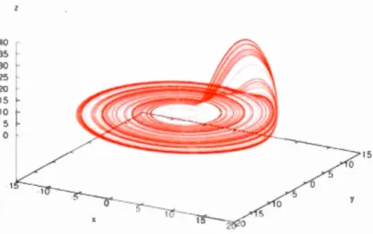
15

0 5

0

Fig. 1 .6 The Chaotic Attractor of Rossi er system visualized in phase space

15

If we examine Figure 1.6, we notice th at the chaotic attractor is composed of a dense collection of points, which seetn to embed a periodic pattern of slightly varying similar orbits that are partially overlapping. The reason behind this partial overlapping of orbits is due to the chaotic nature of the system which gives the chance of any point in a neighborhood of previously visited points of an orbit in the phase space to be visited again by another orbit. This is why these orbits are called: Unstable Periodic Orbits (UPOs ). Th us, a chao tic attractor can simply be defined as a structure th at is composed of infini tel y many UPOs: lt is a dense set of UPOs. U sing methods of Chaos control, we can manipulate the systetn of differentiai equations and make their outcome settle to a single UPO.

Next, we will introduce the equations of the Nonlinear Dynamic State (NDS) Neuron that were derived from the equations of the Rossler system by Alhawarat, in 2007. In addition, we will present the chaos control method that makes the behavior of the NDS neuron settle to a single UPO (Crook et al, 2005).

x/t) = x;(t -1) + b( -y;(t -1)-u;(t -1))

y/t) = Y;(t -1) + c(x;(t -1) + ay/t -1))

n₀,u;(t -1) > 8

u.(t) =

' 'u;(t -1) + d(v + u;(t -1)( -x;(t -1)) + ku;(t -1)) + l;(t),u;(t -1) s 8

where,

a=0.002, b=0.03, c=0.03, d=0.8, v=0.002 and k=-0.057 are constants (Crook et al,

2005, Alhawarat, 2007).

Xi and Yi are considered as the internai variables of a NDS Neuron i.

ui is considered as the voltage output of the NDS Neuron i.

Bis a parameter called the Voltage threshold of ui and is set to O.

no is called: Voltage reset of the NDS neuron (i.e. the value that takes the neuron

voltage ui when the latter bypasses the threshold B). It is a parameter that is set to

-0.7.

The initial conditions of the NDS Neuron i are: xi(O) = 0, yi(O) = 0, ui(O) = no and the

system starts at t = 1.

By comparing the Rossler variables to the NDS Neuron variables, we notice that the

variable z is substituted by u. The reason behind this substitution is simply for

interpreting z as a voltage that is comtnonly prescribed by the letter u in conventional

spiking neuron models.

As we mentioned earlier, neurons communicate with spikes, which encode their

behavioral activity. So, in order to incorporate the spike phen01nenon in the NDS

l

y(t) =

O,u(t) s 8

y is interpreted as the spike output of the neuron which is equal to 1 wh en the neuron

voltage u crosses its threshold ()and 0 elsewhere.

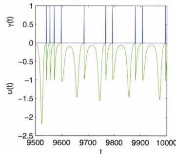
Next, we will visualize a trail of spikes output of the NDS Neuron based on the

variable y that altemates its value as being either 0 or 1 depending on the evolution of u. ..--.. ~ 0.5 -1.5 -2 -2.5 .___ _ ______.... _ _ ___._ _ _ ___.__ _ _ ...__ _ ____J 9500 9600 9700 9800 9900 10000

Fig. 1.7 The NDS Neuron voltage u shown in green color and its spikes output y in blue versus time t.

By examining the output of u and y in figure 1.7, we notice that they don't show any

regularity; this is obvious because the NDS Neuron is a chaotic neuron model. Y et, in

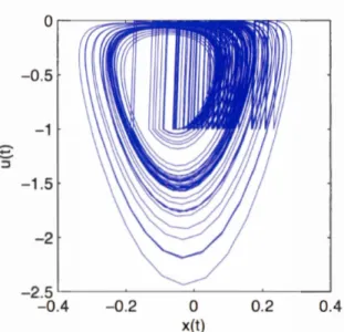
order to visualize the chaotic attractor of the NDS Neuron variables, then we should

plot its phase diagram as we did for the Rossler equations previously. Note that, for

the sake of simplicity, we will show the phase diagram of the NDS Neuron in two

0 -0.5 -1 ... .__.. ::J -1.5 -2 -2.5 -0.4 -0.2 0 0.2 0.4 x(t)

Fig. 1.8 The phase space diagram, in two dimensions, of the NDS Neuron, which shows its chaotic attractor.

Ifwe examine the structure of the chaotic attractor of the NDS Neuron, we notice that

the chaotic attractor of the NDS Neuron is composed of (UPOs). However, the

methods of chaos control can be applied on the variables of a chaotic dynamical system in order to make them settle to a single UPO. For instance, to achieve chaos control in a NDS Neuron and make it settle to a single UPO, we assign its input 1 to its spike output y that occurred r time steps in the past, scaled by a factor w. This is interpreted in mathematical terms, as:

J(t) = wy(t-r)

We can construe the formulation of 1 as the ilnplementation of a self-feedback

connection of the NDS Neuron on itself, which has a time delay that is defined by a parameter r. As for w, it is considered as a degree of freedom interpreted as the weight of this self-feedback connection. This method of chaos control applied to the

1.9 shows an UPO cached by applying SFC and its discrete manifestation in a regular

spikes output pattern of period r. In this example, we choose r to be equal to 100.

0 ~ -0.5 -1 -1.5 L__ -~--~-~---0.2 -0.1 0 x(t) 0.1 0.2 ;;::: 0.5 0 -:;=- -0.5 '5" -1 -1.5

10

ln

in

10

10

Fig. 1.9 Chaos Control: On the left, a settled UPO through chaos control in phase space. On the right, top plot, the discretized version of the UPO shown as a spikes trail ofperiod r = 100 containing 4 spikes. On the right, bottom plot, the evolution of the neuron voltage u.

By varying the initial conditions, the degree of freedom w and/or the delay r we will

theoretically reach an infinite number of different UPOs; discretized by trails of spiking activity of the neuron.

The repertoire of UPOs that can be controlled using the method of chaos control molded in terms of SFC and discretized in spikes patterns can be considered as the vocabulary of the NDS Neuron (Crook et al, 2005). Thus, a discretized version of a

UPO is an expression of a neuronal state of the NDS Neuron. Furthermore, it was

shown that the nmnber of distinct UPOs that can be achieved using chaos control is in the order of hundreds of thousands and is theoretically infinite (Alhawarat, 2007).

In this section, we introduced chaos theory and the NDS Neuron model. Furthermore,

we introduced the main feature of 'states' of the NDS Neuron through chaos control,

extend the concept of states from the synaptic domain to the neuron domain. The NDS N euron is a chaotic spiking neuron mo del and opera tes using ti me delays, which makes it plausible in the field of computational neuroscience. In addition, it satisfies Valiant suggestion because it has theoretically infinitely many states. Next, we will exp lain the theory of chaotic neurodynamics upon which we base our hypothesis.

1.6 Our hypothesis based on stabilization of chaotic attractors

In 1991, Freeman found that wh en an organism (i.e. an animal) is not smelling any odorant, it's brain Electro Encephalogram (EEG) signais activity can be represented in a phase diagram which shows a chaotic attractor, composed of dense orbits with very high degree of irregularity describing a high level of chaos. However, when an familiar odorant is offered to the organism then the attractor, still chaotic, became more regular and constrained to fine orbits, which means that the organism has either leamed the odorant (i.e. cognized the odorant and generated a new memory representation for it) or remembered the odorant (i.e. recognized the odorant by slightly altering its old memory representation). The findings of (Freeman, 1991) are elucidated in the figure 1.10 next:

rab bit is not presented with an odorant, which shows Irregular portrait of neural activity. Right: Phase space, when the rabbit smells food, which seems more ordered and describes a regular portrait of neural activity.

Please check Annex III for a summary and further explanation of Freeman (1991) experiments.

Besides, we showed that an artificial spiking chaotic neural network is able to regularize its chaotic activity when trained with a general class of inputs (Aoun and Boukadoum, 2015). Furthermore, the network was able to discriminate future unknown inputs with the general class of inputs it has learned. Note that the regularization of chaotic activity of the network is manifested by the stabilization of UPOs through out the neurons activity inside the network. Thus, it seems that the regularization of the chaotic attractor, generated by an artificial chaotic spiking neural network, to a more constrained orbit depicting the memory representation of a class of well-defined inputs (Online signatures) as per the authors scope of study (Aoun and Boukadoum, 20 15), could be similar to the dense or bits of a chaotic attractor that are regularized when an organism is faced with a familiar class of stimuli as per the scope of Freeman's experimental study (Freeman, 1991). This comparison between two unrestricted phenomenal representations of memory lays out our hypothesis in considering the representation of memory as a stabilized orbit of a chaotic attractor and leads us to the declaration of our thesis statement in the next section (Section

1. 7).

Finally, we have to mention important research in the literature, which tackles the concept of chaos in the brain. For instance, Tsuda and Kuroda (2001) extend the work of Freeman (1991 ). ln fact, they pro vide a mathematic tnodel, based on chaotic dynatnics, which they cali Cantor coding, that could explain episodic memory (Episodic memory is the ability of the brain to transform short term memory to long