Coastal pollution of the Mediterranean
and extension of its biomonitoring to
trace elements of emerging concern
Faculty of Sciences
Department of Environmental Sciences and Management
Laboratory of Oceanology
Dissertation written by Jonathan Richir
for the fulfilment of the degree of PhD in Sciences
Department of Environmental Sciences and Management Laboratory of Oceanology
Coastal pollution of the Mediterranean and extension of
its biomonitoring to trace elements of emerging concern
Dissertation written for the fulfilment of the degree of Doctor in Sciences at the University of Liège
RICHIR Jonathan
Academic year 2012-2013Supervisors:
Pr J-M. BOUQUEGNEAU, University of Liège Dr S. GOBERT, University of Liège
Jury:
Pr J-M. BECKERS (Jury president), University of Liège Dr K. DAS, University of Liège
Pr G. PERGENT, University of Corte Dr F. SYLVESTRE, University of Namur Pr J-P. THOME, University of Liège
Table of contents:
Remerciements / Aknowledgements ... i
Résumé ... iii
Summary... ... vi
List of abbreviations ... ix
Periodic table of the elements ... xi
Chapitre 1: General introduction
... 11. The sick Ocean ... 1
1.1. Human pressures on oceans ... 1
1.2. The polluted Mediterranean Sea ... 2
2. Trace elements ... 5
2.1. Definition ... 5
2.2. Production and uses ... 6
2.3. Human toxicity... 8
2.4. TEs in the sea: sources and speciation ... ....11
2.5. Removal processes from seawater ... 13
2.6. TE toxicity on marine biota ... 14
2.6.1. TE metabolism and toxicity testing ... 14
2.6.2. TE toxic effects on bivalve molluscs ... 17
2.6.3. TE toxic effects on seagrasses... 19
3. The monitoring of the marine environment ... 21
3.1. “Biomonitoring” ... 21
3.2. “Bioindicators” ... 23
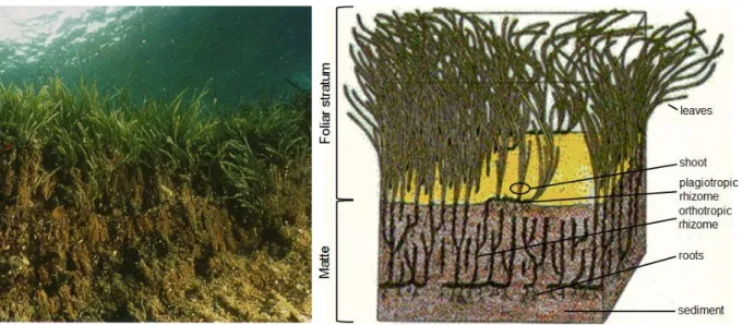
4. Posidonia oceanica ... 24
4.1. A brief description of its biology ... 24
4.1.1. Biogeography ... 25 4.1.2. Morphology ... 26 4.1.3. Ecological roles ... 28 4.2. Seagrasses as bioindicator species ... 29
4.2.1. Posidonia oceanica descriptors ... 29
4.2.2. The choice of proper descriptors ... 31
4. 3. Trace elements bioaccumulation in seagrasses ... 33
4.3.1. Posidonia oceanica as model ... 33
4.3.2. TE balance within Posidonia oceanica ... 35
5. Mytilus galloprovincialis ... 37
5.1. A brief description of its biology ... 37
5.1.1. Biogeography ... 37
5.1.2. General Characteristics ... 39
5.1.3. Reproduction ... 40
5.2. Mytilus spp. as bioindicator species ... 41
5.2.1. Quality indicators ... 41
5.2.2. Pollution monitoring ... 42
5.2.3. Seafood and human health ... 44
5.3. Trace element bioaccumulation in Mytilus galloprovincialis ... 45
5.3.1. Driving factors... 45
5.3.2. Physiological correction ... 46
6. Objectives of the study ... 47
References ... 50
Chapter 2: Spatial variation of TE levels in Posidonia oceanica
... 62Abstract... 62
1. Introduction ... 63
2. Materials and methods ... 64
2.1. Sampling location and design ... 64
2.2. Sample treatment ... 65
2.3. Trace element analysis ... 66
2.4. Statistical analysis ... 66
3. Results and discussion ... 69
3.1. Posidonia oceanica compartmentalization ... 69
3.2. Spatial (temporal) variation of trace element levels ... 71
3.2.2. Sn – Bi ... 72 3.2.3. V ... 73 3.2.4. Mn – Mo ... 73 3.2.5. Ag ... 74 3.2.6. Sb – As – Zn ... 75 3.2.7. Cr – Co – Ni – Cd ... 75 3.2.8. Al – Fe ... 76 3.2.9. Cu ... 77 3.2.10. Pb ... 77 4. Conclusion ... 77 Acknowledgements ... 78 References ... 79 Annex A ... 83 Annex B ... 89 Annex C ... 93 Annex D ... 96
Chapter 3: TE kinetics in Posidonia oceanica
... 99Abstract...99
1. Introduction ... 100
2. Materials and methods ... 101
2.1. Continuous field survey ... 101
2.2. Experimental design... 102
2.3. Posidonia oceanica sample processing ... 106
2.4. Bioavailable trace element concentrations... 107
2.5. Sediment samples collect and processing ... 107
2.6. Trace element analysis ... 108
2.7. Statistical and mathematical analysis... 110
3. Results...111
3.1.1.Posidonia oceanica compartmentalization ... 111
3.1.2.Trace elements in sediments ... 113
3.2. Trace elements in seawater and sediments of mesocosms ... 113
3.3. Posidonia oceanica trace element uptake kinetics ... 114
3.3.1.Moderate contamination ... 114
3.3.2.Acute contamination ... 120
3.3.3.Trace element trapping ... 120
3.4. Posidonia oceanica trace element loss kinetics ... 121
3.4.1.Moderat contamination ... 121
3.4.2.Acute contamination ... 122
3.5.Trace element uptakes by epiphytes ... 123
4. Discussion ... 123
4.1. The Calvi Bay as a reference for the Northwestern Mediterranean ... 123
4.2. Posidonia oceanica natural compartmentalization ... 124
4.3. TE uptake kinetics by P. oceanica ... 126
4.4. TE loss kinetics by P. oceanica ... 130
4.5. Trace element kinetics in rhizomes... 131
4.6. Trace element levels in epiphytes ... 132
Conclusions ... 133
Acknowledgements ... 133
References ... 135
Annex A ... 140
Annex B ... 144
Chapter 4: Influence of physiology on the bioaccumulation of TEs by Mytilus
galloprovincialis
... 152Abstract ... 152
1. Introduction ... 153
2. Material and methods ... 155
2.1. Biological material ... 155
2.2. Sample preparation ... 155
2.4 Mathematical and statistical analysis ... 156
3. Results and Discussion ... 159
3.1. TE concentrations ... 159
3.2. TE concentrations or total contents as a function of mussel weight or shell length... 163
3.3. TE concentrations as a function of shell length ... 166
3.4. TE concentrations as a function of sex ... 169
3.5. TE accumulation and tissue compartmentalization ... 171
4. Conclusion ... 176 Acknowledgements ... 177 References ... 178 Annex A ... 182 Annex B ... 187 Annex C ... 197
Chapter 5: General discussion
... 2021. Context summary ... 202
2. Contamination of the French Mediterranean littoral ... 204
3. The Calvi Bay as a reference site ... 206
4. P. oceanica and M. galloprovincialis trace element bioaccumulation behaviours ... 207
5. Trace element kinetics ... 212
6. Trace element compartmentalization ... 216
Bibliography. ... 220
i
Remerciements – Acknowledgements
Après ces 5 années de thèse … et quelques jours … il m’est agréable de remercier toutes les personnes qui de près ou de loin ont contribué à la réalisation de ce travail.
Je tiens à remercier tout d’abord le Pr. Jean-Marie Bouquegneau : « pourquoi tu ne déposes pas un FNRS ? ». Je vous cite, et vous aviez raison, c’est passé. Je suis très heureux d’avoir pu passer ces 5 dernières années au sein de votre laboratoire ; merci.
Je remercie aussi tout particulièrement le Dr. Sylvie Gobert. J’ai pu bénéficier de sa bienveillance tout au long de ma thèse. On a abattu pas mal de boulot ensemble. Tu m’as permis de réaliser plus de missions de terrain que je ne l’aurais espéré, tu as énormément allongé la liste de mes « contacts » scientifiques, tu as tout fait pour rendre cette thèse la plus agréable et la plus scientifiquement productive possible. Merci enfin pour tes nombreux conseils et le temps que tu as toujours accordé à la relecture de mes publis et travaux. Tout ce travail n’aurait jamais abouti sans les heures passées avec Renzo Biondo sur l’ICP-MS. « Renzo, j’aurais besoin de l’ICP tous les jours du mois à venir, c’est possible ? ». On n’en était pas loin, et on en a vidé des bouteilles d’argon, mais ça en valait la peine. Merci aussi pour ton aide précieuse sur le terrain et pour tous tes bons conseils tout au long de ma thèse. Ce travail, c’est à toi que je le dois en grande partie.
Il me faut aussi tout particulièrement remercier le Dr. Gilles Lepoint. Ça n’a pas dû être facile d’être mon voisin de bureau, surtout quand les parois ne sont pas insonorisées. Tu as toujours répondu à mes nombreuses questions, dans mon bureau ou par panneaux de gyproc
interposés. Et merci aussi pour les heures que tu as passées sous l’eau à m’aider. Merci aussi au Dr. Simon Vermeulen. Il est peut-être le plus méritant de tous les membres du labo, car c’était lui mon collègue de visu. Cinq années de tête à tête, à se prendre la tête sur des questions scientifiques nombreuses et diverses, ce n’est plus de l’amour, c’est de la rage. Mes remerciements vous également à tous les autres membres des labos d’Océanologie et LSD qui m’ont aidé d’une façon ou d’une autre au cours de ces cinq années, ou que j’ai tout simplement côtoyés tous les jours de ma thèse. Pour bon nombre, on avait tous embarqué un peu près en même temps dans la … belle … aventure de la thèse ; le radeau des médusés … . Merci Loic, Dorothée, Krishna, Patrick, Nico, Joseph, Thibaud, François, Christelle, Sarah, Aurélie, Marielaure et Fabienne. Merci aussi à tous mes autres collègues des labos des étages du dessus, du dessous, et des autres bâtiments du Sart-Tilman.
Je tiens aussi à remercier le Dr. Pierre Lejeune, Directeur de la STARESO, et toute son équipe. J’en aurai fait des missions, des dernières missions (aussi nombreuses), et j’ai chaque fois pu largement profiter des infrastructures de la station et des coups de mains de tout un chacun. Comme lieu de travail, y’a pire … . Merci les Staresiens. Merci aussi à Stéphane Sartoretto et collègues de l’IFREMER de Toulon pour leur disponibilité et pour
l’échantillonnage. Un conseil, quand Stéphane vous dit que la mer n’est pas trop belle, mais que ça devrait le faire, prenez deux cachets contre le mal de mer … . Je remercie aussi Mr.
ii Pantallacci, Directeur de la ferme conchylicole de l’Etang de Diane, pour nous avoir
gracieusement offert plus de moules que j’aurais pu en analyser.
Si la recherche scientifique ne coutait rien, ça ferait déjà longtemps qu’on habiterait sur Mars et Total Recall ne serait pas qu’un film. Merci donc aux différents institutions et projets qui ont contribué à fiancer ce travail : le FRS-FNRS (FNRS - ASPIRANTS - 1.A168.08, FRFC 2.4.624.05, FRFC 2.4.502.08), l’Université de Liège (Bourse du Patrimoine, Fonds Spéciaux: crédits classiques et gros équipements), la Communauté Française de Belgique (ARC Race 05/10- 333), l’IFRMER, la Collectivité Territoriale de Corse, l’Agence Française de l’Eau (PACA-Corse) et STARESO: projet STARE-CAPMED.
Il me faut enfin remercier Mr. A. Nackers, mon professeur d’anglais du secondaire, qui a relu la majeure partie de ce travail ; je l’ai réussi, mon examen d’anglais ? Mais aussi Fred et Arnaud ; il est 19h30, et on est toujours en train de peaufiner la mise en page avant l’impression finale aaaaaahhhhhhh !!!!!! Merci à tous les deux.
iii
Résumé
La Méditerranée, mer semi-fermée aux côtes densément peuplées, est soumise à de nombreuses pressions anthropiques, dont la pollution chimique par les éléments traces. Ces polluants, issus de nos activités continentales et transportés par voies fluviales, aériennes, ou directement rejetés dans les eaux côtières, s’accumulent dans le réceptacle final que sont les mers et océans, et touchent tout particulièrement les zones littorales. Dans le courant des années 70, des chercheurs suggérèrent d’utiliser des organismes, plus particulièrement les moules du genre Mytilus, pour évaluer le statut de contamination chimique des écosystèmes littoraux: le biomonitoring était né. Depuis, de très nombreux travaux utilisant diverses espèces animales et végétales ont été publiés.
Deux des indicateurs biologiques, ou bioindicateurs, les plus largement étudiés en Méditerranée sont la magnoliophyte marine Posidonia oceanica, formant de vastes et denses prairies sous-marines appelées herbiers, et la moule méditerranéenne Mytilus galloprovincialis. Les études portant sur ces deux espèces se sont essentiellement intéressées à la contamination par le Cr, le Ni, le Cu, le Zn, le Cd, le Pb (moules et posidonies), le Fe (posidonies), l’As, le V et l’Ag (moules). De nombreux autres éléments traces dont le Be, l’Al, le Mn, le Co, le Se, le Mo, le Sn, le Sb et le Bi n’ont cependant fait l’objet que de peu voir d’aucun suivi écotoxicologique chez ces deux espèces. Or, l’évolution de nos technologies et de nos modes de consommation et la récente augmentation de l’extraction et de la production de ces éléments en réponse aux besoins croissants des pays en voie de développement, font de la pollution environnementale par les éléments traces un sujet d’actualité.
L’objectif global de ce travail était dès lors d’évaluer le potentiel bioindicateur respectif de la posidonie et de la moule méditerranéenne dans le monitoring du Be, de l’Al, du Mn, du Co, du Se, du Mo, du Sn, du Sb, du Bi, du Fe, de l’As, du V, et de l’Ag, éléments pour la plupart catégorisés de “préoccupation environnementale nouvelle”. Le biomonitoring intégré des éléments traces classiquement investigués nécessite un suivi continu de leurs niveaux de concentrations environnementales ; nous avons dès lors également mesurés leurs teneurs dans les deux bioindicateurs sélectionnés.
La posidonie et la moule méditerranéenne se complémentent l’une l’autre dans les études de monitoring de la pollution côtière. Si les deux espèces accumulent les polluants
iv dissouts dans la colonne d’eau, la posidonie, enracinée sur le fond, accumule en outre les polluants stockés à plus long terme dans le sédiment ; la moule, bivalve filtreur, accumule quant à elle les polluants particulaires en suspension dans la colonne d’eau. L’utilisation combinée de ces deux bioindicateurs fournit donc une vue d’ensemble de l’état de santé de l’environnement dont ils sont issus (eau, sédiment, matière en suspension).
Notre premier objectif était de mesurer, à l’échelle du littoral méditerranéen français, la variabilité spatiale des concentrations en éléments traces dans la posidonie et de définir dans quelle mesure les éléments de préoccupation environnementale nouvelle menaçaient l’intégrité chimique des écosystèmes côtiers. Nous avons observé d’une part que la majorité des éléments trace peu/pas étudiés présentaient une variabilité spatiale équivalente ‒ voir supérieure ‒ à celle des éléments classiquement dosés, et que cette variabilité spatiale pouvait être associée à des sources spécifiques de contaminations anthropiques tel que l’agriculture (Mo), l’activité minière (Sb), le stockage et le raffinage de produits pétroliers (V), ou la présence de ports et centres urbains d’importance (Sn, Bi). Leur monitoring, au même titre que celui des éléments traces classiquement suivis en Méditerranée, s’avère dès lors indispensable. De plus, l’étude approfondie de l’état de contamination de la Baie de Calvi, côte nord-ouest de la Corse (France), nous a par ailleurs permis de définir (ou redéfinir) ce site comme site de référence en Méditerranée nord-occidentale pour le monitoring de la pollution chimique par les éléments traces.
Nous nous sommes ensuite intéressés aux mécanismes physiologiques d’accumulation, de stockage et d’excrétion des éléments traces chez la posidonie. La contamination in situ de portions d’herbier permit de modéliser les cinétiques d’accumulation rapide des contaminants par la posidonie. Les compartiments de la plante répondirent différemment à l’exposition aux polluants. Ainsi, les feuilles âgées et sénescentes de la plante assimilèrent moins rapidement les contaminants que les jeunes feuilles en croissance. Les éléments traces, une fois accumulés, pouvaient ensuite être redistribués entre les différents compartiments de la plante, notamment vers le système rhizomes-racines du sédiment jouant ainsi le rôle d’archive biologique. Après l’arrêt des contaminations, les cinétiques de décontamination des faisceaux de feuilles furent relativement rapides et dépendaient notamment du temps d’exposition aux éléments traces, de leur caractère essentiel ou toxique et du compartiment suivi. La posidonie s’avère donc être un bioindicateur sensible pour le monitoring de la pollution côtière par les éléments traces présente et passée.
v Nous avons montré que la moule méditerranéenne accumulait efficacement les éléments traces, tant ceux de préoccupation environnementale nouvelle que ceux classiquement étudiés chez ce bioindicateur. De même que pour la posidonie, la physiologie de la moule conditionne sa réponse à l’exposition aux polluants. Ainsi, son cycle reproductif dilue, lors de la production massive de gamètes, les concentrations en éléments traces, et conduit à des différences plus ou moins marquées entre individus de sexes opposés. Le caractère conservatif de la distribution des éléments traces entre les différents compartiments corporels des individus suggèrent une importante régulation physiologique de leurs niveaux internes. Enfin, la taille des moules utilisées dans le présent travail, issues de l’aquaculture, n’influence que peu les concentrations interindividuelles, toutes les moules d’un même lot ayant approximativement le même âge.
En conclusion, le présent travail a permis d’améliorer et d’élargir l’état des connaissances relatives au monitoring de la pollution par les éléments traces, en particulier par des éléments peu étudiés de préoccupation environnementale avérée, via l’utilisation des deux principaux bioindicateurs utilisés en Méditerranée, soit la posidonie et la moule méditerranéenne.
vi
Summary
The Mediterranean Sea, a semi-enclosed sea with densely populated coasts, is submitted to numerous anthropogenic pressures: among them, the chemical pollution by traces elements. These pollutants, coming from our continental activities, are transported through rivers or by air and accumulate in seas and oceans where they mainly affect coastal areas. During the 70ies, scientists suggested to use organisms, in particular mussels of the genus Mytilus, in order to evaluate the status of chemical contamination of coastal ecosystems. Biomonitoring was born. Since, many monitoring studies were published using various animal and vegetal species.
Two of the most studied bioindicators species in the Mediterranean are the marine magnoliophyte Posidonia oceanica and the Mediterranean mussel Mytilus galloprovincialis. Monitoring studies with these two species have mainly focussed on contaminations by Cr, Ni, Cu, Zn, Cd, Pb (Mytilus galloprovincialis and Posidonia oceanica), Fe (Posidonia oceanica), As, V and Ag (Mytilus galloprovincialis). However, other trace elements like Be, Al, Mn, Co, Se, Mo, Sn, Sb and Bi have been subject to nearly no ecotoxicological survey. Furthermore the worldwide evolution of our technologies and of our lifestyle increases the extraction and production of trace elements (notably to answer needs of developing countries). The biomonitoring of the pollution by trace elements is henceforth a topical subject.
The overall objective of this work was therefore to evaluate the potential use of Mytilus galloprovincialis and Posidonia oceanica as bioindicators to monitor the Mediterranean coastal pollution by Be, Al, Mn, Co, Se, Mo, Sn, Sb, Bi, Fe, As, V, and Ag. These trace elements, mostly little studied, can be categorized as elements of “environmental emerging concern”. A time-integrated efficient monitoring of trace elements requires the continuous survey of their environmental levels; we therefore also measured levels of trace elements classically monitored with these two species.
Mytilus galloprovincialis and Posidonia oceanica complement each other in monitoring surveys. Both species accumulate pollutants dissolved in the water column. Posidonia oceanica, rooted in the seafloor, accumulates moreover pollutants stored in sediments in the long term. Mytilus galloprovincialis, as a filter feeder, further accumulate particulate pollutants suspended in the water column. The combined use of both bioindicators
vii therefore provides a global view of the health status of the coastal environment (water, sediments, suspended matter).
Our first goal was to measure, at the scale of the French Mediterranean littoral, the spatial variability of trace element contents in Posidonia oceanica, and to determine if trace elements of environmental emerging concern threaten the chemical integrity of coastal ecosystems. We observed that the large majority of trace elements little or no monitored with Posidonia oceanica showed an equivalent to higher spatial variability than elements classically monitored with that species. We also showed that the spatial variability could be associated to specific anthropic activities like agriculture (Mo), mining (Sb), storage and refinement of oil products (V), or the presence of harbours and major urban centres (Sn, Bi). Their monitoring, along with the one of trace elements classically studied in the Mediterranean, turns out to be essential. In addition, the in-depth study of the contamination state of the Calvi Bay (Northwestern coast of Corsica, France), enabled us to define (or re-define) this site as a reference site for the monitoring of the chemical pollution by trace elements in the Northwestern Mediterranean.
We further studied the physiological mechanisms of accumulation, storage and excretion of trace elements by Posidonia oceanica. In situ contamination of seagrass bed portions allowed us to model the rapid kinetics of accumulation of contaminants by Posidonia oceanica shoots. Compartments of the plant answered differently to pollutant exposures. So, adult and senescent leaves assimilated pollutants less rapidly than young actively growing leaves. Trace elements, once accumulated, could be redistributed between the plant compartments, notably towards the rhizomes-roots systems buried in sediments. Our results experimentally showed that these below-ground organs could therefore play the role of biological archives for many elements. At the end of periods of exposure to pollutants, kinetics of decontaminations of Posidonia oceanica shoots were relatively fast and depended notably on the duration of the exposure to trace elements, on their toxic or essential character and on the studied compartment. We concluded that Posidonia oceanica was a sensitive bioindicator for the monitoring of the past and present coastal pollution by trace elements.
We showed that Mytilus galloprovincialis efficiently accumulated trace elements of environmental emerging concern as well as elements classically studied with this bioindicator species. The physiology of mussels further conditioned their answers to pollutant exposures. Their reproductive cycle dissolved trace element concentrations during the massive
viii production of gametes and conducted to differences more or less important between individuals of both sexes. The conservative character of the distribution of trace elements between the different body compartments of Mytilus galloprovincialis suggested an important physiological regulation of their internal levels. Finally, the size of mussels used in this study, harvested from an aquaculture farm, did not noticeably influence inter-individual concentrations, all mussels of a same rope having approximately the same age.
In conclusion, this study enabled to improve and enlarge our state of knowledge about the monitoring of the pollution of the Mediterranean coastal environment by trace elements. In particular, both Mytilus galloprovincialis and Posidonia oceanica showed to be good candidates for the monitoring of trace elements of environmental emerging concern.
ix
List of abbreviations
3IL: 3rd Intermediate Leaves
ASTM: American Society for Testing and Materials BAL: Blades of Adult Leaves
BiPO: Biotic index using Posidonia oceanica BQE: Biological Quality Element
CGDD: Commissariat Général au Développement Durable CI: Condition Index
COT: Committee on Toxicity of Chemicals in Food, Consumer Products and the Environment CRM: Certified Reference Material
DGT: Diffusion Gradient in Thin Films DL: detection limit
DM: dry matter
DNA: deoxyribonucleic acid DOC: dissolved organic carbon
DRC ICP-MS: Inductively Coupled Plasma Mass Spectrometry using Dynamic Reaction Cell technology
EC50: the median effect concentration EDTA: ethylenediaminetetraacetic acid EEA: European Environment Agency
EPA: United States Environmental Protection Agency ERL: effects range-low
ERM: effects range-median
EROD activity: Ethoxyresorufin-O-deethylase activity Fm: maximum fluorescence
Fm’: light-adapted maximal fluorescence Fv: variable fluorescence
GSH: glutathione
GST: glutathione S-transferase HC: Health Canada
IFREMER: Institut Français de Recherche pour l'Exploitation de la Mer LC: critical limit
LC50: the median lethal concentration LD: detection limit
LQ: quantification limit MN: micronucleus
mRNA: messenger ribonucleic acid NRR: neutral red retention
OIL: Other Intermediate Leaves PACA: Provence-Alpes-Côte d’Azur
PAM fluorometry: pulse amplitude modulation fluorometry PAM: Plan d'Action pour la Méditerranée
x PNUE: Programme des Nations Unies pour l’Environnement
PoCMT1: one member of the Posidonia oceanica chromomethylase (CMT) family POMI: Posidonia oceanica multivariate index
PoMT2k: Posidonia oceanica Metallothionein (MT) 2k PREI: Posidonia oceanica rapid easy index
PSII: photosystem II
SAL: Sheaths of Adult Leaves SnTBT: tin as tributyltin species
STARESO: Station de Recherche Océanographiques et sous-marines TBT: tributyltin
TE: trace element
TSS: total suspended solids
TT Action Level: Treatment Technique Action Level UN: United Nations
USSG: United States Geological Survey WFD: Water Framework Directive WHO: World Health Organization
WSH deaths: deaths from unsafe water, sanitation and hygiene
Chapter 1
-
1
1. The sick Ocean
1.1. Human pressures on oceans
Such as terrestrial ecosystems, marine ecosystems are submitted to increasing anthropogenic disturbances. Land-based activities affect the runoff of pollutants and nutrients into coastal waters and remove, alter, or destroy natural habitats, while ocean-based activities extract resources, add pollution and change species composition (Halpern et al. 2008).
Fig. 1. Global map (A) of cumulative human impact across oceans. Insets: highly impacted regions in the Eastern Caribbean (B), the North Sea (C), and the Japanese waters (D) and one of the least impacted regions, in northern Australia and the Torres Strait (E) (modified after Halpern et al. 2008).
On the basis of expert judgment, Halpern et al. (2007, 2008) recently mapped the impact of 17 anthropogenic drivers of ecological change (e.g. pollution, fishing, ocean acidification, species invasion etc.) on marine ecosystems (Fig. 1), combined into a single comparable estimate of cumulative human impact (6 levels, from very low to very high impact). Their analysis indicated that no area is unaffected by human influence, and a large
2 fraction (41% of the oceans) is strongly affected (from medium high to very high scores) by multiple drivers. However, some large areas of relatively little human impact still remain (3.7% of the oceans), particularly near the poles were seasonal or permanent ice limits human access.
These increasing pressures upon the marine realm threaten ecosystems, especially seabed biotopes (Salomidi et al. 2012). The ecologic, economic and social importance of marine ecosystems being irrefutable (Costanza et al. 1997, Salomidi et al. 2012), a well-planned approach of managing the marine space is essential to achieve sustainability (Salomidi et al. 2012). Otherwise, entire ecosystems will stop functioning under their actual form, as is the case for the highly productive hotspots of biodiversity that are coral reefs (Hughes et al. 2003), which is likely to lead to the complete loss of goods and services derived from these ecosystems (Worm et al. 2006).
1.2. The polluted Mediterranean Sea
The intense human activities, particularly in coastal areas surrounding the enclosed and semi-enclosed seas, always lead in the long term to important environmental impacts which are reflected in the form of a marine and coastal degradation and an increase of the risk of more important damages (Papathanassiou and Gabrielides 1999). The Mediterranean is one of the richest regions of Europe in terms of diversity of marine species with a high rate of endemism (Bianchi and Morri 2000). In the Mediterranean, coastal ecosystems are dominated by macrophytes (magnoliophytes and algae; Boudouresque 2004), a globally net autotrophic system displaying many ecological benefits (e.g. primary production, habitats, source of food and oxygen, carbon well, stabilization of sediments etc.; Levin et al. 2001). Despite their environmental, economic and social importance, a growing number of reports document the occurring regression and/or ecofunctional changes of these ecosystems (e.g. Occhipinti-Ambrogi and Savini 2003, Ardizzone et al. 2006, Boudouresque et al. 2006)
3 Fig. 2. Pollution hot spots (full red circles) along the Mediterranean coasts (EEA 2006).
Pressures suffered by the Mediterranean (e.g. pollution hot spots, Fig. 2) make it a vulnerable ecological unit (Turley 1999). This sea is of too small dimensions to ecologically self-counterbalance. The point of saturation of the pollutants discharged in the Mediterranean, whose area is the 35th of that of the Atlantic, will be more quickly achieved than in the oceans. In addition, the almost total absence of tide does not allow the dilution of pollutants and prevents the natural phenomena of depuration as encountered in larger bodies of water (i.e. in oceans). The Mediterranean also shows a deficiency in the movement of its deep water masses, and of its surface currents which "turn in circles" in this almost closed basin. As well, the answer of the Mediterranean to environmental disturbances is more rapid than in the larger oceans (Augier 2010). These specificities make therefore of the Mediterranean a privileged site of study of pressures and changes performed by men on the environment, and announced the scenarios that we could live on in the future in all the oceans of the world (Bethoux et al. 1999).
Major environmental problems along the French Mediterranean coasts are caused by river transported pollution, treated industrial and urban wastewater and intense urbanisation along its densely populated coastline. Areas of environmental concern are shown in Fig. 3; their major corresponding anthropogenic activities are listed below: • Marseilles and Nice are
4 relatively big coastal cities (density > 3000 persons per km2) discharging mostly treated urban wastewater into the sea; • river Rhône transports significant loads of nutrients and other pollutants (organic matter, trace elements) from its drainage basin; • in the area of Fos-Étang de Berre are located the biggest French and the second largest European harbour hosting oil and methane terminals, as well as a large industrial complex; • rivers Hérault and Gard are considered as vectors of industrial pollution (hydroelectric and nuclear plants, petroleum processing, electronic, metal plants and chemicals); • in harbours of Marseilles, Sète, Port-la-Nouvelle, Port-Vendres, Toulon, Nice, Bastia and Ajaccio, petroleum hydrocarbon pollution occurs because of deballasting practices and accidental oil spills (EEA 2006).
Fig. 3. Zoom on the Mediterranean coastlines of France. Full red circles: pollution hot spots; blue full circles: areas of major concern; full black squares: coastal cities (modified from EEA 2006).
As regards trace elements, the high levels currently measured in the Mediterranean indicate non-stationary geochemical cycles which result from an increase of external inputs (Saliot 2005). Effectively, although trace elements are present naturally in the environment, their current concentrations observed in coastal waters are linked to the growth of industrial, agricultural and urban activities since the early sixties (e.g. Bethoux et al. 1990, PNUE/PAM 2009). These anthropogenic activities generate the introduction of a considerable amount of chemicals in the marine coastal ecosystem; these substances show toxic properties likely to
5 cause multiple damage at the level of organisms, populations and ecosystems (Nordberg et al. 2007, Amiard 2011).
2. Trace elements
2.1. Definition
According to the International Union of Pure and Applied Chemistry (McNaught and Wilkinson 1997), trace elements (TEs) are any element having an average concentration of less than about 100 parts per million atoms (ppma) or less than 100 µg.g-1 (Fig. 4). Such a precise definition does not exist in earth sciences, because the concentration of an element in a given phase can be so low that it is considered a trace element, whereas the same element can constitute a main part of another phase (e.g. Fe and Al; Navratil and Minarik 2011).
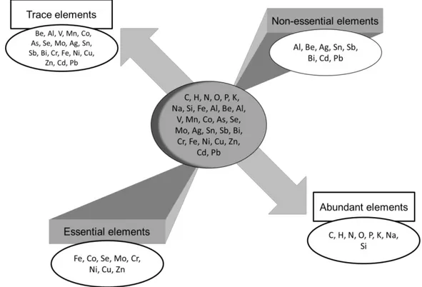
Fig. 4. Essential and non-essential elements, abundant or in traces (modified after Amiard 2011).
Previously, scientists used the generic term "heavy metals" when referring to trace elements. Today this appellation is discussed. Effectively, some metals are not particularly "heavy" (e.g. Al, Ni). In addition, some elements are not metals (e.g. As, Se). For these
6 reasons, the majority of researchers prefer today the name "metallic trace elements" (if it is indeed metals) to the appellation "heavy metals", or then the formula "trace elements" when they are not metals (As, Se, B) (Duffus 2002).
Trace elements can either be essential or non-essential (Fig. 4); the essential elements recognized by the World Health Organization (WHO) are I, Zn, Se, Fe, Cu, Cr and Mo, the latter playing an important role in biological systems (WHO 1996, 2004). Others TEs may/could also be essential, such as Mn, Co, As, Ni, V etc; the essentiality is a characteristic which evolves according to our knowledge and to the sensitivity of the authors who have a propensity more or less strong to classify an element among the essential or not (Amiard 2011). Non-essential TEs such as Hg, Pb or Cd play no physiological role, and are often toxic even in very small quantity (Nordberg et al. 2007). For these non-essential TEs, only a threshold of toxicity exists, while essential TEs can be either deficient in too small quantities, either toxic when they are absorbed in high concentrations (Amiard 2011).
2.2. Production and uses
If the world refinery and mine production of some trace elements (e.g. As, Cd, Pb, Sn) has proportionally little evolved since the 80ies, most of them have known a substantial increase (e.g. Fe, Al, Mo), particularly since the beginning of years 2000 (Table 1, Fig. 5). World demand for minerals is affected by 3 general factors: (i) uses for mineral commodities, (ii) the level of population that will consume these mineral commodities, and (iii) the standard of living that will determine just how much each person consumes (Kesle 2007).
Today, with the integration of India, the People’s Republic of China and other populous developing and emerging countries (e.g. Brazil and Russia) into the world economy, more than 50 % of the world’s population (instead of the previous 20 %) account for the largest part of raw materials consumption (Tiess 2010); alone, the People’s Republic of China’s demand for Al, Pb, Cu, Ni, Zn and Sn accounted for 32 ± 5 % of the world consumption in 2008 (Sievers et al. 2010). This increasing demand for mineral raw materials further concerns numerous “emerging” elements. These elements can either be truly emerging as they have just gained entry to the environment or because they are “contaminants of emerging concern” (Daughton 2004, 2005), as is the case for V, Sb or Bi.
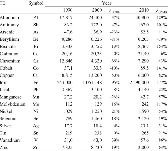
7 TE Symbol Year 1990 2000 ↗(1990) 2010 ↗(1990) Aluminum Al 17.817 24.400 37% 40.800 129% Antimony Sb 83,2 122,0 47% 167,0 101% Arsenic As 47,6 36,9 -23% 52,8 11% Beryllium Be 0,286 0,226 -21% 0,203 -29% Bismuth Bi 3,333 3,752 13% 8,467 154% Cadmium Cd 20,16 20,23 0% 21,40 6% Chromium Cr 12.846 4.320 -66% 7.290 -43% Cobalt Co 37,1 33,3 -10% 89,5 141% Copper Cu 8.815 13.200 50% 16.000 82% Iron Fe 543.000 1.061.148 95% 2.590.000 377% Lead Pb 3.367 3.100 -8% 4.140 23% Manganese Mn 27,2 20,2 -26% 42,7 57% Molybdenum Mo 112 129 16% 242 117% Nickel Ni 1.029 1.250 21% 1.590 54% Selenium Se 1.789 1.460 -18% 2.120 19% Silver Ag 17,7 18,4 4% 23,1 31% Tin Sn 219 238 9% 265 21% Vanadium V 31,0 43,0 39% 57,6 86% Zinc Zn 7.325 8.730 19% 12.000 64%
Table 1. World production of 19 trace elements of concern for the years 1990, 2000 and 2010, and percentage of increase by decades (data compiled from the Mineral Yearbooks published by the US Geological Survey website, http://www.usgs.gov/).
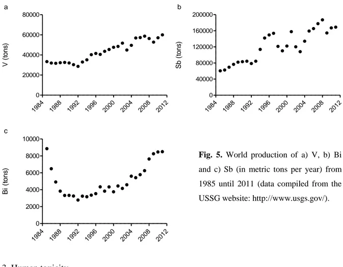
The use of these contaminants of emerging concern are multiple and diverse. V is regarded as one of the hardest of all metals. Since 1992, the world production of has V increased by 50 % per decade (Fig. 5a). This ubiquitous TE is employed in a wide range of alloys for numerous commercial applications extending from train rails, tool steels, catalysts, to aerospace (Moskalyk and Alfantazi 2003).
Antimony, whose mine production was 3 times higher in 2011 than in 1985 (Fig. 5b), greatly increases the hardness and the mechanical strength of lead, and is found in batteries, antifriction alloys, type-metal, small arms and tracer bullets, and cable sheathing. It further has many uses as a flame retardant (in textiles, papers, plastics and adhesives), as a paint pigment, ceramic opacifier, catalyst, mordant and glass decolouriser, and as an oxidation catalyst (Filella et al. 2002, Shtangeeva et al. 2011).
8 Bismuth consumption deeply decreased during the second half of the 80ies (Fig. 5c), mainly because of a decline in usage by the chemical and pharmaceutical industries. Nowadays, Bismuth is anew largely consumed in low-melting alloys and metallurgical additives, including electronic and thermoelectric applications. The remainder is used for catalysts, pearlescent pigments in cosmetics, pharmaceuticals, and industrial chemicals (Fowler and Sexton 2007).
1984 1988 1992 1996 2000 2004 2008 2012 0 20000 40000 60000 80000 a V ( to n s ) 1984 1988 1992 1996 2000 2004 2008 2012 0 40000 80000 120000 160000 200000 b S b ( to n s ) 1984 1988 1992 1996 2000 2004 2008 2012 0 2000 4000 6000 8000 10000 c B i (t o n s )
Fig. 5. World production of a) V, b) Bi and c) Sb (in metric tons per year) from 1985 until 2011 (data compiled from the USSG website: http://www.usgs.gov/).
2.3. Human toxicity
The major exposure media to TEs for humans are food, water and air (Beckett et al. 2007). The whole human kind needs water for sustaining life; the provision of a safe drinking water supply is a high priority issue for safeguarding the health and well-being of humans (Van Leeuwen 2000, WHO 2011) and is an important development issue at national, regional and local levels (WHO 2011). Although standards legislate the acceptable levels of contaminants in drinking water (Table 2), the supply of quality water remains a major challenge for humanity in the twenty-first century (Fig. 6; Schwarzenbach et al. 2010).
9 Fig. 6. Deaths from unsafe water, sanitation and hygiene (WSH) estimated by WHO sub-region for year 2000 (WHO 2002).
The spectrum of adverse effects caused by the consumption of contaminated water is huge and ranges from relatively harmless to life threatening (Table 2; Van Leeuwen 2000). Inorganic As is present in groundwater used for drinking in several countries all over the world (e.g. Bangladesh, Chile and China). Populations exposed to As via drinking water show excess risk of mortality from lung, bladder and kidney cancer, the risk increasing with increasing exposure. There is also an increased risk of skin cancer and other skin lesions, such as hyperkeratosis and pigmentation changes (Järup 2003).
Japanese who consumed Cd polluted rice and river water over a period of 30 years were found to have accumulated in their bodies a large amount of Cd that lead to a serious osteoporosis-like bone disease known to the Japanese as “itai–itai byo” or “ouch–ouch disease” (Pan et al. 2010). Industrial wastes and agriculture activities have released hazardous and toxic materials in the groundwater and thereby led to the contamination of drinking water of some of the great Cairo cities, Egypt. Strong relationships between contaminated drinking water and chronic diseases were identified: renal failure was related to Pb and Cd contaminations, liver cirrhosis to Cu and Mo, hair loss to Ni and Cr, and chronic anaemia to Cu and Cd (Salem et al. 2000).
Al WHO: 0.9 (< 0.1 in conventional
treatment plants; < 0.2 in other
treatment types)
Erosion of natural deposits; Al salts used as flocculents during the treatment of drinking water. Little indication that orally ingested Al is acutely toxic to humans; no adverse health effect at levels found in drinking water; Al exposure is a risk factor for the development or acceleration of onset of Alzheimer
disease. Sb WHO: 0.020; EPA, HC: 0.006 Erosion of natural deposits; discharge from petroleum refineries; fire retardants; ceramics;
electronics; solders; contaminants from pipes and fittings.
Increase in blood cholesterol; decrease in blood sugar; microscopic changes in organs and tissues (thymus,
kidney, liver, spleen, thyroid). As WHO, EPA: 0.01 Erosion of natural deposits (erosion and weathering of soils, minerals, ores); runoff from
orchards; runoff from glass and electronics production wastes.
Skin damage or problems with the circulatory system; increased risk of getting cancer (lung, bladder, liver,
skin - classified as human carcinogen); neurological effects (numbness and tingling of extremities).
Be WHO: 0.010; EPA: 0.004 Discharge from metal refineries and coalburning factories; discharge from electrical, aerospace
and defense industries.
Intestinal lesions; rarely found in drinking-water at concentrations of health concern.
Bi No guideline value Concentrations of Bi in drinking water have not been reported. Doses used in medicines are very much larger than the estimated dietary exposure; dietary exposures to Bi
are unlikely to be of toxicological concern. Cd WHO: 0.003; EPA, HC: 0.005 Erosion of natural deposits; corrosion of galvanized pipes; discharge from metal refineries;
runoff from waste batteries and paints; leaching from solders or black polyethylene pipes;
industrial and municipal waste.
Kidney damage; softening of bone; classified as human carcinogen.
Cr WHO, HC: 0.05; EPA: 0.010 Erosion of natural deposits; releases or spills from industrial uses (steel and pulp mills). Enlarged liver; irritation of the skin, respiratory and gastrointestinal tracts; kidney problems.
Co No guideline value Drinking water has a low-Co content, usually between 0.0001 and 0.005 ppm. Cardiovascular effects (cardiogenic shock, sinus tachycardia, left ventricular failure, and enlarged hearts) observed in people who consumed large amounts of beer over several years time containing Co sulfate as a
foam stabilizer; gastrointestinal effects (nausea, vomiting, and diarrhea), effects on blood, liver injury, and
allergic dermatitis have also been reported in humans from oral exposure to Co.
Cu WHO: 2;
EPA: TT Action Level = 1.3;
HC ≤ 1.0
Erosion of natural deposits (erosion and weathering of rocks and minerals); corrosion of household plumbing systems; contaminants from pipes and fittings; acidic mine water drainage; landfill leachates; sewage effluents; iron-related industries.
Short term exposure: gastrointestinal distress; long-term exposure: liver or kidney damages. Cu is an essential element in human metabolism; adverse health effects occur at levels much higher than the aesthetic
objectives. Fe HC: aesthetic objectives ≤ 0.3 Erosion of natural deposits (erosion and weathering of rocks and minerals); use of Fe
coagulants; corrosion of steel and cast iron pipes.
Not of health concern at levels causing acceptability problems in drinking-water.
Pb WHO, HC: 0.010;
EPA: TT Action Level = 0.015
Erosion of natural deposits; corrosion of plumbing systems (pipes, solders, brass fittings and lead service lines); contaminants from pipes and fittings.
Infants and children (under 6 years): delays in physical or mental development; neurobehavioural effects; children could show slight deficits in attention span and learning abilities. Adults: Kidney problems; high blood pressure. Others: anaemia; central nervous system effects; in pregnant women, can affect the unborn child; classified as probably carcinogenic to humans.
Mn WHO: 0.4;
HC: aesthetic objectives ≤ 0.05
Erosion and weathering of rocks and minerals; naturally occurring in many surface water and
groundwater sources, particularly in anaerobic or low oxidation conditions (the most important source for drinking-water).
Not of health concern at levels causing acceptability problems in drinking-water.
Mo WHO: 0.02 Contaminations may occur in areas where Mo ore is mined. Occurs in drinking-water at concentrations well below those of health concern. Ni WHO: 0.07 Ni levels in natural waters ranges from 0.002 to 0.010 ppm in fresh and tapwater; water is
generally a minor contributor to the total daily oral intake; the Ni contribution from water may
be significant where there is heavy pollution, where there are areas in which Ni occurs naturally in groundwater or where there is use of certain types of kettles of non-resistant material in wells or of water that has come into contact with Ni-plated taps; released from
fittings; released from industrial Ni deposits.
Lack of evidence of a carcinogenic risk from oral exposure to Ni.
Se WHO: 0.04; EPA: 0.05; HC: 0.01 Naturally occurring (erosion and weathering of rocks and soils); discharge from petroleum and metal refineries; discharge from mines.
Toxic effetcs: hair or fingernail losses at extremely high levels of exposure; numbness in fingers or toes;
circulatory problems. Ag WHO: available data inadequate to
permit derivation of health-based
guideline value; EPA: 0.1
Naturally occurring (erosion and weathering of rocks and soils); drinking water, not treated
with Ag for disinfection purposes, usually contains extremely low concentrations of Ag.
Water-soluble Ag compounds such as nitrate have a local corrosive effect and may cause fatal poisoning if swallowed accidentally.
Sn No guideline value Drinking-water is not a significant source of Sn; increasing use of Sn in solder, which may be used in domestic plumbing, and proposed for use as a corrosion inhibitor.
Occurs in drinking-water at concentrations well below those of health concern; excessive levels of Sn in
canned beverages or other canned foods has been acute gastric; no evidence of adverse effects in humans
associated with chronic exposure to Sn.
V No guideline value Typical values of V concentrations in drinking water are below the detection limit. The main source of V intake is food; V little absorbed in the gastro-intestinal tract and mainly eliminated
unabsorbed with the faeces. Zn HC: aesthetic objectives ≤ 0.05 Naturally occurring; industrial and domestic emissions; leaching may occur from galvanized
pipes, hot water tanks and brass fittings; Zn concentrations in water from active or inactive
mines can be substantial.
Not of health concern at levels found in drinking-water; effects on human health by contamination on water supplies must be rare.
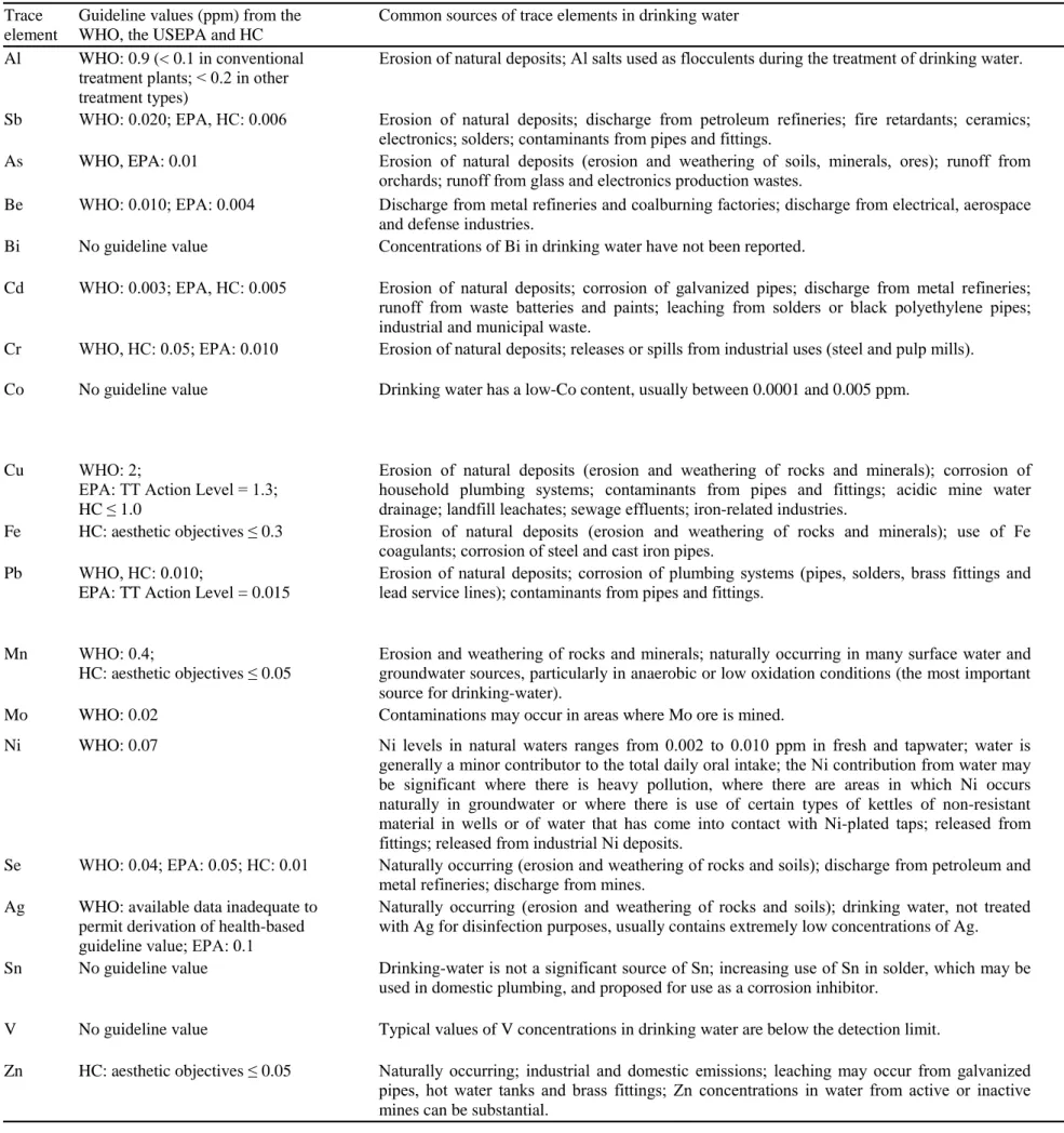
Table 2. Trace element guildeline values (ppm) for drinking water, common sources of trace elements in water and potential effects on human health. Data compiled from the World Health Organization (WHO, 2011), the United States Environmental Protection
Agency (EPA, 2009), Health Canada (HC, 2012), Nordberg et al. (2007) and the Committee on Toxicity of Chemicals in Food, Consumer Products and the Environment (COT, 2008). Treatment Technique (TT) Action Level: US drinking water requiring a treatment process in order to reduce the level of a contaminant.
11 Essential micronutrient may also show toxic effects when ingested at too high levels, as reviewed by Goldhaber (2003) and widely detailed in Nordberg et al. (2007). The ingestion of very high doses of Cr causes liver and kidney problems. Abdominal pain, cramps, nausea, diarrhea, and vomiting have been caused by the consumption of beverages containing high levels of Cu, and liver damage has been seen in individuals with diseases of Cu metabolism. Although exposure to Mn is not of health concern at levels causing acceptability problems in drinking-water, the consumption of Mn-containing well water has caused lethargy, tremor, and mental disturbances in Japan, and neurologic symptoms were reported in individuals exposed to Mn-contaminated drinking water in Greece.
The rivers, estuaries, coastal seas and oceans form an ecological continuum where pollutants pass in transit (CGDD 2011). According to the United Nations (UN 2004), more than 80 % of the pollution of the seas comes from inland via the rivers or through runoff and discharges from the coastal areas. As at least 60 % of the world’s population live within 100 km of the coast, the contaminations of coastal waters may pose serious risks to human health as well as marine ecosystems (Tanaka 2006). It is therefore essential to monitor the chemical pollution of coastal areas.
2.4. TEs in the sea: sources and speciation
Continental runoff and atmospheric deposition are the primary inputs of TEs in the marine environment (Callender 2003): crustal material is either weathered on (dissolved) and eroded from (particulate) the Earth’s surface or injected into the Earth’s atmosphere by volcanic activity; forest fires and biogenic sources are of a lesser importance (Nriagu 1989, 1990). In addition to these natural sources, there exists a multitude of anthropogenic emission sources, the major ones resulting from mining and smelting activities. Mining releases metals to the fluvial environment as tailings and to the atmosphere as metal-enriched dust whereas smelting releases metals to the atmosphere as a result of high-temperature refining processes (Callender 2003). Other important land-based anthropogenic sources of TEs proceed from various municipal, industrial and agricultural activities (Tanaka 2006). The occurrence of TEs in effluents stemming from notorious anthropogenic sources is summarized in Table 3.
12 Table 3. Occurrence of trace elements in effluents and associated land-based human sources (modified after Nagajyoti et al. 2010).
Trace elements are present in seawater under different oxidation states and chemical forms including free solvated ions, inorganic complexes (e.g. with Cl-, OH-, CO32-, SO42- etc.), organometallic compounds and organic complexes (e.g. with phytoplankton metabolites, proteins, humic substances etc; Donat and Bruland 1994). This distribution of elements amongst defined chemical species is termed “speciation” (Templeton et al. 2000). Speciation affects bioavailability, and bioavailability is determined by both external environmental conditions and the physiological/biological characteristics of organisms (Chapman 2008).
Addressing the chemical form of an element instead of its total concentration renders thenceforth the gained information much more valuable. The underlying reason for this is that the characteristics of just one species of an element may have such a radical impact on living systems (even at extremely low concentrations) that the total element concentration becomes of little value in determining its impact. A good example is Sn: the inorganic form of this element is much less toxic (or even does not show toxic properties), but the alkylated form is highly toxic (Cornelis and Nordberg 2007).
13 2.5. Removal processes from seawater
Unlike organic pollutants which can be degraded to less harmful components by biological or chemical processes, TEs are considered as non-degradable pollutants (Navratil and Minarik 2011, Pan and Wang 2012). This persistent character of TEs can alter, sometimes quite strongly, their natural biogeochemical balance in contaminated environments (Doney 2010). Processes removing TEs from seawater include active biological uptake or passive scavenging onto either living or non-living particulate material (Bruland and Lohan 2003). From the biological point of view, the most important uptake pathway is the mass transport through plasma membrane (Ahlf et al. 2009).
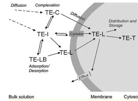
TEs are mainly transported into biological cells in ionic form due to the fact that ionic channels are involved (Fig. 7). In addition, specific transport mechanisms cross the membrane barrier like binding with membrane carrier proteins or transport through hydrophilic membrane channels. Lipid-soluble (non-polar) metal forms, including alkyl-TE compounds and neutral, lipophilic, inorganically complexed TE species can cross biological membrane by diffusion. TEs bound to very fine particles can also be engulfed by endocytosis (McGeer et al. 2004, Ahlf et al. 2009). Following absorption, metals are transported to internal organs for utilization, storage, toxic effects, and possibly release (Ahlf et al. 2009).
Fig. 7. Conceptual model of the main processes and sources for uptake of trace elements at a biological membrane. TE-C: TE complex; TE-I: TE ion; TE-LB: labile particle-bound TE; TE-L : TE bound to a biological ligand; TE-T : TE at target site (modified after Worms et al. 2006)
TEs can be removed from seawater through passive adsorption onto a wide variety of relatively high affinity surface sites on both living and dead particulate material (Bruland and
14 Lohan 2003). The combined process of surface adsorption, followed by particle settling, is termed scavenging (Goldberg 1954, Turekian 1977). Thereafter, labile bound TEs can also be desorbed from particles and resupply free metal ions to the dissolved metal pool (Fig. 7; Ahlf et al. 2009).
Much of the particulate material (along with its associated TEs) is internally recycled either in the water column or in surficial sediments. Marine sediments are usually considered as the ultimate sink of TEs where they can heavily accumulate (Bruland and Lohan 2003); marine sediments can also act as a source of TEs by releasing chemicals back to the overlying water column (Burton 2010, Pan and Wang 2012). The primary flux processes between sediments and the water column are resuspension and deposition, bioturbation, advection, upwelling/downwelling, diagenesis reactions, and diffusion (Burton 2010). Because of these remobilization processes, the effects of metal pollution on local environments and organisms can be substantial and long lasting in spite of years of restoration efforts (Pan and Wang 2012).
2.6. TE toxicity on marine biota
2.6.1. TE metabolism and toxicity testing
The potential impacts of contaminants on aquatic biota depend on the total concentrations of the contaminant, its speciation, interactions at receptors sites (e.g. at a fish gill membrane or on an algal cell surface), and uptake into the organism/cell, with either subsequent adverse effects or intracellular detoxification (Batley et al. 2004). Thenceforth, the sole exposure to a TE does not harm an organism; it has to be both absorbed and retained in sensitive portions of its life structure in toxic amounts (Chapman 2008).
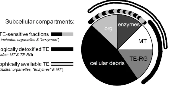
The toxicity of each TE is related to a metabolically available threshold concentration (Rainbow 2002). TEs accumulated by biota occur in a bioreactive fraction that is metabolically active and available, and a fraction that has been detoxified and is unavailable (Fig. 8; Chapman 2008). TEs bound to inducible TE-binding proteins such as metallothionein or phytochelatin or precipitated into insoluble concretions consisting of TE-rich granules comprise biologically detoxified TEs, whereas TEs bound to sensitive fractions such as
15 organelles and heat-sensitive proteins can be metabolically active; the higher the proportion of TE-sensitive fractions, the greater the vulnerability to TE toxicity (Wallace et al. 2003, Wallace and Luoma 2003). The TE-sensitive fractions and TE bound to metallothionein represent TE available for trophic transfer to predators (Wallace and Luoma 2003). This compartmentalization of metal as defined by Wallace and Luoma (2003) and Wallace et al. (2003) is a useful tool to interpret multiple ecotoxicological consequences of the subcellular partitioning of metals within organisms.
Fig. 8. A generalized ecotoxicological pie chart depicting subcellular compartments based on the biological significance of the various subcellular fractions in clams. Clams were homogenized, and differential centrifugation and tissue digestion techniques were used to obtain the following subcellular fractions (detailed procedure in Wallace and Luoma, 2003): TE-rich granules (TE-RG), cellular debris, organelles (org), heat-sensitive proteins (“enzymes”) and heat-stable proteins (metallothioneins, MT). Subcellular fractions that are potentially vulnerable to TE exposure (i.e. organelles and “enzymes”; dashed arc) constitute TE-sensitive fractions. Those fractions that are involved with TE detoxification (i.e. metallothionein, MT, and TE-rich granules, TE-RG; solid arc) constitute biologically detoxified TE. Fractions containing TE that is readily available to predators (i.e. organelles, “enzymes” and MT; double arc) constitute trophically available TE (modified after Wallace et al. 2003).
Mayer-Pinto et al. (2010) critically reviewed studies done on effects of TEs on aquatic assemblages and/or populations of invertebrates. These authors selected a sub-set of papers; the selection was done using an explicit randomisation process to ensure that a representative sample was taken from the scientific literature. Results from this random selection brought
16 out that most studies in the field had been descriptive: they generally demonstrated that the diversity of an assemblage tends to decrease with an increase of TE concentrations and that there are differences in the structure of the assemblages in the presence of large concentrations of TEs. Such descriptive studies are, however, unable to demonstrate any causal relationship between the TE contamination and the changes in the assemblages (Mayer-Pinto et al. 2010).
Toxicity testing methods are therefore required as a tool for predicting and assessing the impacts of anthropogenic environmental stressors on organisms and ecosystems (Amiard 2011). Laboratory-based toxicity testing has the obvious advantage to be unaffected by habitat or natural disturbances. This allows for experimental evaluation of various parameters and conditions, such as temperature, toxicant threshold effect levels, mixture interactions, life stages, and exposure duration under strictly controlled conditions (Burton 2010). Despite laboratory studies show lethal and sub-lethal effects of TEs on organisms, extrapolating such findings to the field is little reliable (Ralph et al. 2006): the majority of contaminant exposures of aquatic organisms are episodic in nature due to changing water and sediment quality; in addition, physicochemical characteristics of aquatic ecosystems (e.g., temperature, pH, water hardness and dissolved organic carbon) greatly influence bioavailability, toxicity, and bioaccumulation of contaminants (Chappie and Burton 2000, Liber et al. 2007, Clements et al. 2012). Naturally occurring factors in water and sediments affecting TE chemical bioavailability cannot be easily simulated in the laboratory (Lewis and Devereux 2009). Additional field experiments are therefore necessary to validate laboratory results under relevant environmental conditions.
Complementary results from laboratory and field toxicity tests are useful for decision making, particularly if the responses of the test organisms are severe and occur in multiple species (Burton 2010). Within this perspective, detailed reviews on tested organisms from different taxonomic groups allow (i) to identify species that may be suitable candidates in a suite of toxicity test protocols, keeping in mind regional differences in species requirements and tolerances (Fairbrother et al. 2007), and (ii) to highlight knowledge gaps that require to be addressed (van Dam et al. 2008). Such a work of synthesis was recently performed for the coastal waters of northern Australia, recognised internationally as important strongholds for marine biodiversity and containing some of the least impacted marine habitats in the world
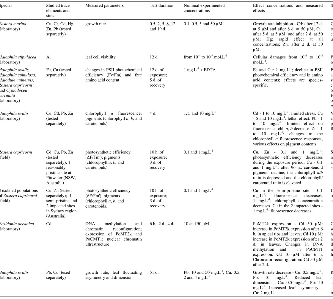
17 (Fig. 1; Halpern et al. 2008): Van Dam et al. (2008) reviewed the state of the science for toxicity testing methods for water column contaminants, summarizing data available for 16 taxonomic groupings, among them vascular plants (seagrasses and mangroves) and bivalve molluscs; Adams and Stauber (2008) reviewed concomitantly the status of whole sediment toxicity tests developed with numerous species of 7 taxonomic groupings, of which bivalve molluscs. The 2 following paragraphs will focus on TE toxic effects assessed on seagrasses and bivalves molluscs.
2.6.2. TE toxic effects on bivalve molluscs
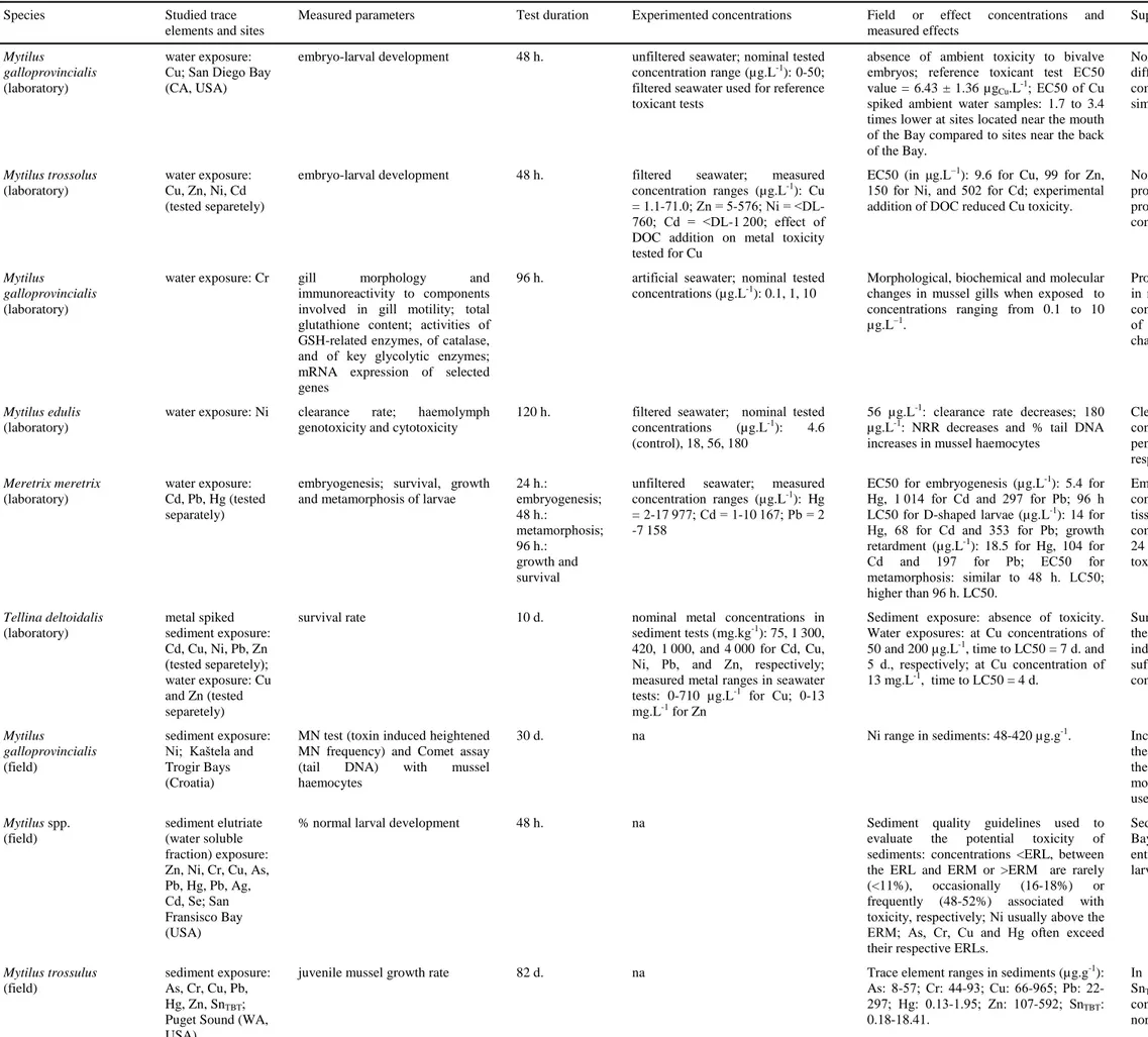
Bivalve molluscs possess many physiological attributes (sensitive to contaminants, tolerant of a wide range of abiotic factors, easily cultured and maintained in laboratory etc.) that render them suitable for consideration as bioassay organisms for toxicity testing (Depledge and Hopkin 1995). They are moreover good accumulators of organometallic contaminants and TEs from their surrounding environment due both to their behaviour and mode of feeding (Bryan et al. 1985). A number of standardized toxicity test protocols have been developed for determining toxicity of single chemicals, complex effluents and ambient samples of water or sediment to marine bivalves (e.g. Cal/EPA 2004, Burton 2010; detailed guidance manuals available from the EPA and the American Society for Testing and Materials, ASTM). Toxicity tests established on bivalve embryo-larval development are among the most sensitive in the EPA’s national toxicity dataset, which is used to derive water quality criteria (Rosen et al. 2005). Among bivalve molluscs, mussels from the genus Mytilus have been largely used.
TE toxicity on bivalve molluscs can be determined at different structural levels, from genes to individuals, and response parameters have included, in addition to larval-embryo developments, changes in growth rates, clearance rates and survival rates, DNA-damages, or changes in tissue morphology and in specific component immunoreactivity (Table 4). Toxicity varies greatly between TE. The median effects concentrations (EC50) for Meretrix
meretrix embryogenesis is 188 higher for Cd than for Hg. Moreover, this difference in
toxicity directly relies upon the response parameter of interest; so, the EC50 for M. meretrix larval growth is only 6 times higher for Cd than for Hg (Wang et al. 2009).