Salient object detection and segmentation in videos

HAL Id: tel-02299316

https://tel.archives-ouvertes.fr/tel-02299316

Submitted on 27 Sep 2019

HAL is a multi-disciplinary open access

archive for the deposit and dissemination of sci-entific research documents, whether they are pub-lished or not. The documents may come from teaching and research institutions in France or

L’archive ouverte pluridisciplinaire HAL, est destinée au dépôt et à la diffusion de documents scientifiques de niveau recherche, publiés ou non, émanant des établissements d’enseignement et de recherche français ou étrangers, des laboratoires

Salient object detection and segmentation in videos

Qiong Wang

To cite this version:

Qiong Wang. Salient object detection and segmentation in videos. Signal and Image processing. INSA de Rennes, 2019. English. �NNT : 2019ISAR0003�. �tel-02299316�

T

HESE DE DOCTORAT DE

L’INSA

RENNES

COMUE UNIVERSITE BRETAGNE LOIRE ECOLE DOCTORALE N° 601

Mathématiques et Sciences et Technologies de l'Information et de la Communication

Spécialité : Signal, Image, Vision

Par

Qiong WANG

Salient object detection and segmentation in videos

Thèse présentée et soutenue à Rennes, le 09 MAI 2019

Unité de recherche : Univ Rennes, INSA Rennes, CNRS, IETR (Institut d'Electronique et de Télécommunication de Rennes), UMR6164

Thèse N° : 19ISAR 07 / D19 - 07

Rapporteurs avant soutenance :

Frederic DUFAUX

Directeur de recherche CNRS – CentraleSupelec Guangtao ZHAI

Professeur - université de Shanghai Jiao Tong

Composition du Jury :

Président :

Didier COQUIN

Professeur des universités - université de Savoie Mont Blanc

Membres du jury :

Frederic DUFAUX

Directeur de recherche CNRS – CentraleSupelec Guangtao ZHAI

Professeur - université de Shanghai Jiao Tong Olivier LE MEUR

Maître de conférences HDR - université de Rennes 1

Directeur de thèse :

Kidiyo KPALMA

Professeur des universités - INSA Rennes Co-encadrante de thèse :

Lu ZHANG

Intitulé de la thèse :

Salient object detection and segmentation in videos

Qiong WANG

En partenariat avec :

A

CKNOWLEDGEMENT

I would like to express my sincere gratitude towards my thesis advisors, Prof. Kidiyo KPALMA and Prof. Lu ZHANG. Thanks for providing me the opportunity to work with them, discussing the problems during the research, reviewing my reports, papers and thesis carefully, giving me many suggestions, encouragement and support.

I would like to thank my committee members, Prof. Didier COQUIN, Prof. Frederic DUFAUX, Prof. Guangtao ZHAI and Prof. Olivier LE MEUR. Thanks for their helpful comments and suggestions.

I also thank Prof. Sylvain GUEGAN for the helpful comments during intermediate defense.

My appreciation also goes to my colleagues from the laboratory VAADER team of IETR, INSA Rennes for the pleasure time. I would also like to acknowledge the people for sharing their knowledge.

I would like to express my special grateful to China Scholarship Council (CSC) for the financial supporting. I would like to thank my husband, parents and brother for their love.

R

ÉSUMÉ ÉTENDU

Introduction

Le système visuel humain a une capacité efficace à reconnaître facilement des régions d’intérêt dans des scènes complexes, même si les régions ciblées ont des couleurs ou des formes similaires à l’arrière-plan. La détection d’objets saillants (SOD) vise à détecter l’objet saillant qui attire le plus l’attention visuelle. La réponse d’un système SOD est une carte de saillance dans laquelle chaque pixel est étiqueté par une valeur réelle prise dans l’intervalle [0,1] pour indiquer sa probabilité d’appartenir à un objet saillant. Plus la valeur est élevée, plus la saillance est élevée.

En fonction de l’objectif visé, les approches existantes peuvent être classées glob-alement en deux catégories: les approches basées image et les approches basées vidéo. Les approches basées image modélisent le processus de vision en fonction de l’apparance de la scène. Le système visuel humain étant sensible aux mouvements, les approches basées vidéo détectent l’objet saillant en utilisant des indices, à la fois, du domaine spatial que du domaine temporel et deviennent de plus en plus popu-laires. Dans ce travail, nous nous concentrons sur les approches basées vidéo. Ce su-jet a montré beaucoup d’intérêt notamment pour des applications exploitant l’attention humaine, telle que la conduite autonome [98], l’évaluation de la qualité, surveillance militaire, etc.

En conduite autonome, l’un des principaux problèmes est de garantir la robustesse de reconnaissance des panneaux de signalisation. Ces panneaux sont généralement de couleurs vives et attirent facilement l’attention humaine. Les approches de détection d’objets saillants dans une vidéo permettent de détecter le panneau de signalisation dans une scène dynamique, ce qui contribue à améliorer la sécurité lors de la conduite autonome.

Dans l’évaluation de la qualité d’image, la sensibilité du système visuel humain à divers les signaux visuels est importante. La détection d’objets saillants et l’évaluation de la qualité d’image sont toutes deux liées à la façon dont le système de visuel hu-main perçoit une image; les chercheurs intègrent des informations de saillance à des

modèles d’évaluation de la qualité d’image visant à améliorer leur performance. Une méthode habituelle consiste à utiliser la saillance comme une fonction de pondération pour refléter l’importance (ou la saillance) de la région dans une image.

Une autre application peut être trouvée dans la surveillance militaire. Les objets tels que les humains, les voitures et les avions attirent généralement un grand intérêt et doivent être soigneusement observé. Pour capter l’évolution de ces objets spécifiques, le calcul de la saillance fournit un indice important pour localiser les objets cibles.

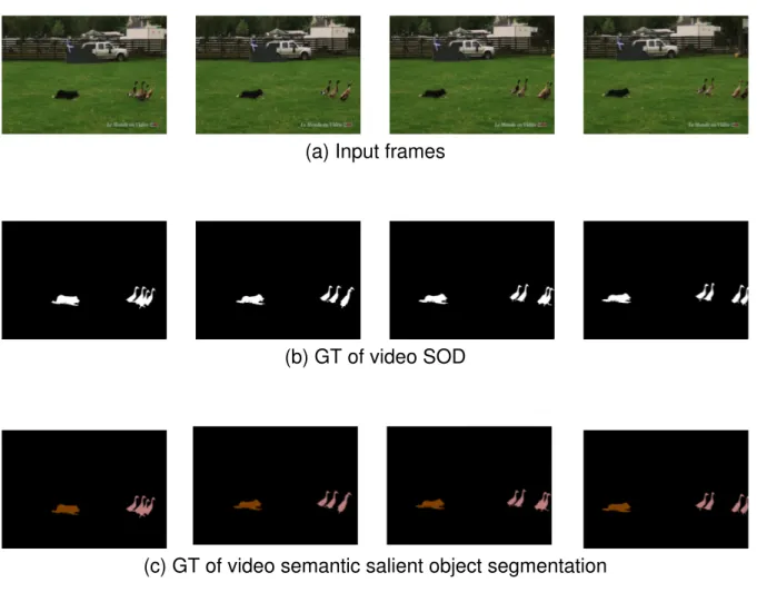
Les méthodes de calcul de saillance basées vidéo insistent uniquement sur l’étiquetage de chaque pixel de l’image vidéo en indiquant “saillant” ou “non saillant”. Pour les scènes réelles, la région saillante détectée peut contenir plusieurs objets (voir Fig.R1 (b)). Décomposer une région saillante en un ensemble d’objets différents est plus sig-nificatif et meilleur pour la compréhension de la vidéo. La Fig.R1 (c) montre la seg-mentation sémantique d’objets vidéo saillants [42] où tous les objets de même éti-quette sémantique sont regroupés sous cette étiéti-quette. Sur la Fig.R1 (d), on peut voir la segmentation semi-supervisée utilisant un étiquettage manuelle initial pour faire la segmention à travers la vidéo. L’assistance humaine est adoptée pour définir les ob-jets d’intérêt qui sont généralement délimités dans la première image de la séquence. En propageant les étiquettes définies manuellement sur le reste de la séquence de la vidéo, l’instance de l’objet d’intérêt est segmentée dans l’ensemble de la séquence vidéo. La segmentation semi-supervisée d’objets vidéo peut être considérée comme un problème de suivi, mais avec le masque en sortie. Dans la carte en sortie, les pixels sont regroupés en plusieurs ensembles auxquels sont attribués une identité cohérente à l’objet: les pixels d’un même ensemble appartiennent au même objet.

Ce dernier type de segmentation s’avère plus attractif mais n’a pas encore été complètement étudié et donc laisse de la place pour la recherche. Ainsi cette thèse s’est également intéressée à la segmentation semi-supervisée d’objets vidéo.

Notions de base sur la détection d’objets vidéo saillants

Lors de la création de jeux de données, de longues vidéos sont collectées par des volontaires ou sélectionnées à partir de sites Web de partage de vidéos comme Youtube. Ensuite, la fixation visuelle humaine est collectée pour une séquence vidéo d’entrée. A l’aide d’un système de eye-tracking, les participants aux expériences visualisent tous les courts vidéo-clips et les points de leur fixations sont enregistrés. Puis, tous les

Première image Images d’entrée (a)

(b) Vérité terrain (GT) d’objets vidéo saillants

(c) GT d’objets saillants basée sémantique

Etiquetage manuel GT pour la segmentation semi-supervisée de l’objet vidéo

(d)

Figure R1. Comparaison entre la détection d’objets saillants, la ségmentation séman-tique d’objets saillants et la segmentation semi-supervisée d’objets saillants

masques d’objets sont annotés manuellement dans chaque image par les participants. Enfin, l’objet vidéo saillant est défini à l’échelle de la vidés entière: l’objet qui conserve les densités de fixation les plus élevées tout au long de la vidéo est sélectionné comme

objet saillant et la vérité-terrain est ainsi générée.

Dans le cadre de cette étude, cinq jeux de données ont été exploitées : VOS [49], Freiburg-Berkeley Motion Segmentation (FBMS) [8, 63], Fukuchi [27], DAVIS 2016-val [68] et DAVIS-2017-val [69]. Diverses métriques sont utilisées pour mesurer la simi-larité entre la carte de saillance générée (SM) et la vérité-terrain (GT). Les mesures couramment utilisées [6] sont: erreur absolue moyenne (MAE), courbe de précision-rappel (P-R), mesure de F-measure, précision-rappel et précision.

Techniques traditionnelles de déctection d’objets vidéo

saillants

Selon les techniques utilisées, les méthodes de détection d’objets vidéo saillants peu-vent être grossièrement scendées en deux catégories: méthodes les traditionnelles et les méthodes utilisant l’apprentissage profond.

Dans cette étude, une nouvelle méthode traditionnelle de détection des objets sail-lants dans les vidéos est proposée. Les méthodes traditionnelles de détection d’objet basées sur l’a priori de l’arrière-plan peuvent rater des régions saillantes lorsque l’objet saillant touche les bords de l’image. Pour résoudre ce problème, nous proposons pour détecter la totalité de l’objet saillant d’ajouter les bordures virtuelles. Un filtre guidé est ensuite appliqué sur la sortisaillance temporelle en intégrant les informations de bor-dure spatiale pour une meilleure détection des objets saillants du bord. Enfin, une carte de saillance spatio-temporelle globale est obtenue en combinant la carte de saillance spatiale et la carte de saillance temporelle en fonction de l’entropie. Les principales contributions sont:

• une technique basées sur la notion de bordure virtuelle est proposée pour dé-tecter un objet saillant connecté au bord de l’image,

• un filtre sensible aux contours est introduit pour fusionner les contours spatiaux avec les informations temporelles afin d’améliorer les contours des objets sail-lants,

• une nouvelle façon de décider du niveau de confiance de la carte de saillance spatiale et de la carte de saillance temporelle par le calcul de l’entropie et l’écart-type.

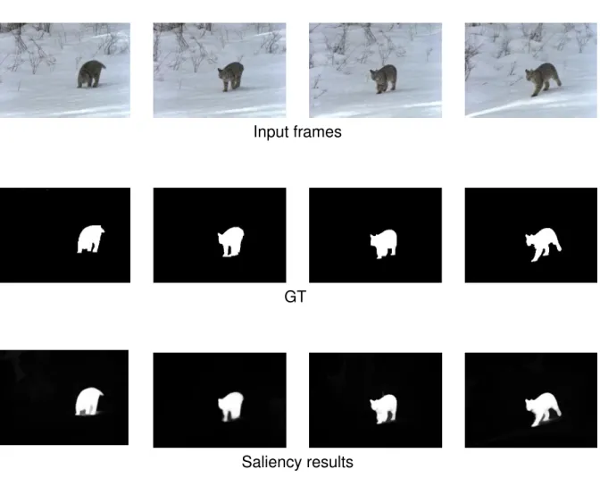
La Fig.R2 montre un des exemples de cartes de saillance générées à l’aide de la nouvelle approche VBGF exploitant les bords virtuels et le filtre guidé pour la détection d’objets vidéos saillants et la vérité-terrain (GT) correspondante.

Images d’entrée

Vérité terrain

Cartes de saillance générées

Figure R2. Exemples de cartes de saillance générées avec la méthode proposée (VBGF).

Revue des méthodes utilisant l’apprentissage profond

pour la détection des objets saillants dans les vidéos

Ces dernières années, les méthodes d’apprentissage profond (ou deep-learning) ont considérablement amélioré la détection des objets saillants dans les vidéos. C’est un sujet important et il reste encore beaucoup à explorer. Il est donc intéressant de se faire une idée globale, sur les méthodes existantes, qui pourrait ouvrir la voie à des

travaux futurs. Les méthodes basées sur l’apprentissage profond peuvent atteindre des performances élevées, mais elles sont largement dépendantes des jeux de données d’apprentissage. Il est donc nécessaire de tester la générécité des méthodes de l’état de l’art en effectuant des comparaisons expérimentales sur différents jeux de données publics. Ainsi, nous donnons un aperçu des développements récents dans ce domaine et comparons les méthodes correspondantes à ce jour. Les principales contributions sont:

• un apperçu des méthodes récentes d’apprentissage profond pour la détection d’objets saillants dans les vidéos,

• un classement des méthodes de l’état de l’art ainsi que leur architecture,

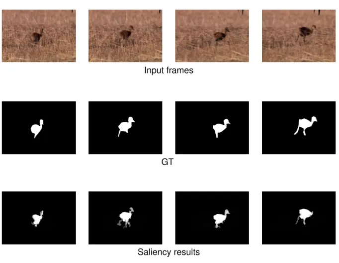
• une étude expérimentales comparative pour tester la générécité des méthodes de l’état de l’art à travers des expérimentations sur des bases de données publiques. Afin de montrer comment la performance d’un modèle traditionnel de détection d’objets vidéo saillants peut être encore améliorée en intégrant une méthode d’apprentissage profond, une méthode étendue (VBGFd) est proposée. C’est la version élargie de la méthode traditionnelle VBGF proposée intégrant la technique de deep-learning. La Fig.R3 montre exemples de cartes de saillance générées par la méthode proposée (VBGFd).

Méthode deep-learning pour la segmentation semi-supervisée

de l’objet vidéo

Dans le domaine de segmentation semi-supervisée de l’objet vidéo, la technique de déformation de masque, qui adapte (recale) le masque de l’objet cible en fonction du flux de vecteurs entre images consécutives, est largement utilisée pour extraire l’objet cible. Le gros problème de cette approche est que la carte déformée générée n’est pas toujours d’une grande précision, l’arrière-plan ou d’autres objets pouvant être détectés à tort comme étant l’objet cible. Pour remédier à ce problème, nous proposons une méthode SWVOS, qui utilise la sémantique de l’objet cible comme guide lors du pro-cessus de recalage. Le calcul du taux de confiance de déformation détermine d’abord la qualité de la carte déformée générée. Ensuite, une sélection de la sémantique est

Images entrées

Vérité terrain

Cartes de saillance générées

Figure R3. Exemples de cartes de saillance générées par la méthode proposée (VBGFd).

introduite pour optimiser la carte à faible taux de confiance, où l’objet cible est identifié, à nouveau, à l’aide de l’étiquette sémantique de l’objet cible. Les contributions sont:

• une méthode est proposée pour déterminer le niveau de confiance des cartes de recalés,

• la sémantique des objets est introduite pour filtrer les objets du premier plan appartenant à des classes différentes de celle de l’objet prédéfini.

La Fig.R4 montre certaines cartes de segmentation générées par l’approche proposée SWVOS.

Première image et étiquettes générées manuellement

Image d’entrée

Résultats de la segmentation

Figure R4. Exemples de segmentations obtenues à l’aide de la méthode proposée (SWVOS).

Conclusion et perspectives

Cette thèse porte sur les problèmes de détection d’objets vidéo saillants destinée à la séparation des objets saillants de l’arrière-plan dans chaque image d’une séquence vidéo et les problèmes de segmentation semi-supervisée de l’objet vidéo qui visent à attribuer une dentité d’objet cohérente à chaque pixel de chaque image d’une séquence vidéo. Nous avons proposé une méthode traditionnelle de détection d’objets vidéo saillants et une revue des méthodes deep-learning pour la détection d’objets vidéo saillants. Nous avons égalment introduit une extension de la méthode traditionnelle proposée pour y intégrer le deep-learning et une méthode de deep-learning pour la segmentation semi-supervisée de l’objet vidéo. Les approches proposées ont été éval-uées sur les jeux de données publics à grande échelle et difficiles. Les résultats ex-périmentaux obtenus montrent que les approches proposées donnent des résultats

satisfaisants.

Certains travaux futurs peuvent être dérivés des analyses précédentes: utiliser des représentations plus riches les achitectures de deep-learning qui pourraient améliorer les performances l’approche VBGFd proposé; entrainer les réseaux de deep-learning pour la fusion de cartes de saillance pour améliorer l’approche VBGF proposée qui peut faillir quand les saillance temprelles et spatiales ne sont pas suffisamment nettes. On peut également, envisager à employer plus d’indices de saillance vidéo prenant en compte l’attention visuelle humaine. Il sera aussi intéressant d’explorer davantage les aspects temporels et spatio-temporels qui permettraient d’assurer une detection de saillance tout le long de la vidéo. essayez des réseaux faiblement supervisés. Enfin, on peut envisager d’explorer les réseaux faiblement supervisés. En effet, les mod-èles supervisés améliorent les performances de détection, mais reposent sur un jeu de données volumineux d’apprentissage. Les modèles faiblement supervisés qui ne demandent de grandes masses de données retient l’attention et constituent un sujet d’intérêt pour l’avenir.

T

ABLE OF

C

ONTENTS

Introduction 19

Background . . . 19

Overview of the thesis . . . 22

1 Basic knowledge 27 1.1 Procedure of dataset building . . . 27

1.2 Benchmarking datasets . . . 27

1.3 Evaluation metrics . . . 30

2 Traditional techniques for salient object detection in videos 33 2.1 An overview of state-of-the-art methods . . . 33

2.1.1 Classification based on low-level saliency cues . . . 33

2.1.2 Classification based on fusion ways . . . 35

2.2 Introduction of some existing issues . . . 39

2.2.1 Background prior . . . 39

2.2.2 Spatial and temporal information fusion . . . 42

2.3 Virtual Border and Guided Filter-based (VBGF) algorithm . . . 49

2.3.1 Spatial saliency detection . . . 49

2.3.2 Temporal saliency detection . . . 53

2.3.3 Spatial and temporal saliency maps fusion . . . 57

2.4 Experiments and analyses . . . 58

2.4.1 Contributions of each proposed component to the performance . 59 2.4.2 Comparison of the proposed method with state-of-the-art methods 65 2.4.3 Computation time comparison . . . 72

2.5 Conclusion . . . 72

3 Overview of deep-learning methods for salient object detection in videos 75 3.1 Summary of existing surveys and benchmarks . . . 75

3.2 Introduction to state-of-the-arts methods . . . 76 17

TABLE OF CONTENTS

3.2.1 Classification based on the deep representations generation . . 76

3.2.2 Description of salient object detection frameworks . . . 77

3.3 Experimental evaluation . . . 87

3.3.1 Detailed performance on each dataset . . . 88

3.3.2 Global performance on various datasets . . . 96

3.3.3 Computation time comparison . . . 100

3.3.4 Failure cases and analysis . . . 100

3.4 Extension of the proposed method to integrate deep-learning technique 100 3.4.1 Extension of VBGF (VBGFd) . . . 102

3.4.2 Experiments and analysis . . . 102

3.5 Conclusion . . . 106

4 Deep-learning method for semi-supervised video object segmentation 107 4.1 An overview of state-of-the-art methods . . . 107

4.1.1 Online-offline learning . . . 107

4.1.2 Mask warping . . . 108

4.2 Introduction of the existing issue . . . 108

4.3 Semantic-guided warping for semi-supervised video object segmenta-tion (SWVOS) algorithm . . . 111

4.3.1 Mask warping . . . 111

4.3.2 Warping confidence computation . . . 112

4.3.3 Semantics selection . . . 113

4.4 Experiments and analyses . . . 116

4.5 Conclusion . . . 116

5 Conclusion and perspective 119

List of Abbreviations 123

List of Publication 125

Bibliography 127

List of Figures 139

I

NTRODUCTION

Background

The human vision system has an effective ability to easily recognize regions of interest from complex scenes, even if the focused regions have similar colors or shapes as the background. Salient object detection (SOD) aims to detect the salient object that attracts the most the visual attention. The output of the SOD is a saliency map, in which each pixel is labeled by a real value within the range of [0,1] to indicate its probability of belonging to a salient object. Higher value represents higher saliency.

According to the goal of detection, existing approaches can be broadly classified into image SOD or video SOD, which are illustrated in Fig.0.1 and Fig.0.2 respectively.

Input image

Ground truth (GT)

Figure 0.1: Examples of image SOD.

Image SOD models the visual processing based on the appearance of the scene. Since the human vision system is sensitive to motions, video SOD detects the salient object using cues in both spatial domain and temporal domain. In this present work,

Introduction

Input frames

GT of the corresponding frame Figure 0.2: Examples of video SOD.

we focus on video SOD. This topic has gained much attention for its wide applications, especially where the task is driven by the human attention, such as autonomous driving [98], quality assessment, military surveillance, etc.

In autonomous driving, one of the biggest issue is to ensure the robustness of road signs recognition. Road signs are generally in brightly colors and easily catch the human attention. The video salient object detection is good at discovering the road sign in a dynamic scene, which helps to improve the safe during autonomous driving.

In image quality assessment, the sensitivity of the human visual system to various visual signals is important. As salient object detection and image quality assessment are both related to how human vision system perceives an image, researchers incor-porate saliency information to image quality assessment models aiming at improving their performance. One usual way is to adopt salient object detection as a weighting function to reflect the importance region in an image.

Another application can be found in military surveillance. The objects such as hu-mans, cars and airplanes usually attracts a lot of interests and need to be carefully observed. To grasp the trend of these specific objects, video salient object detection provide a useful cue to localize target objects.

For video SOD (see Fig.0.3 (b)), in which the pixels with high value represent salient objects, and the pixels with zero value represent background. There is trend to solve this problem from traditional method to deep-learning based method.

Tradi-Introduction

(a) Input frames

(b) GT of video SOD

(c) GT of video semantic salient object segmentation

(d) GT of video object instance segmentation

Figure 0.3: A comparison of video SOD, video semantic salient object segmentation and video object instance segmentation.

tional methods usually detect the salient object based on hand-crafted features and prior assumptions, while deep-learning methods detect the salient object based on deep representations which are learned from training datasets with provided ground truth. For a given database, deep-learning methods have a better performance than many recent traditional methods. But it should be trained with huge and rich training

Introduction

datasets, which is impossible for some applications where the available data is small. Traditional methods do not suffer from such limitation. Therefore, we firstly focus on video SOD based on traditional method, i.e., detecting salient object based on prior assumption. Deep-learning methods attract large attention for its high accuracy and efficiency. We secondly focus on video SOD based on deep learning methods.

The aforementioned video SOD methods put emphasis on only labeling each pixel in the video frame to be “salient” or “non-salient”. For real-world scenes, the detected salient region may contain multiple objects (see Fig.0.3 (b)). Decomposing the detected region into different objects is more meaningful and is better for video understanding. Video semantic salient object segmentation [42], as show in Fig.0.3 (c), segments the salient region based on the semantic label, in which the salient objects belonging to the same semantic label are grouped together. From Fig.0.3 (d), in the output map of video object instance segmentation, the pixels are grouped into multiple sets and assigned to consistent object IDs. Pixels within the same set belong to the same object.

Video object instance segmentation attracts more interests and has not been fully investigated. We address the problem of assigning consistent object IDs to objects instance. One popular way for video object instance segmentation is called as Semi-supervised video object segmentation. Human-guidance is adopted to define the ob-jects that people want to segment. It is usually delineated in the frame that the object appears in the first time. By propagating the manual labels to the rest of the video sequence, the object instance is segmented in the whole video sequences. Semi-supervised video object segmentation can be regarded as a tracking problem but with the mask output.

Overview of the thesis

The thesis is organized as in Fig.0.4. Chapter 1 introduces the preliminary knowledge about saliency detection. Chapter 2 is dedicated to a proposed traditional approach for video SOD, and an overview of recent deep-learning based methods and an extended model are proposed for video SOD in Chapter 3. In Chapter 4, a semi-supervised video object segmentation approach is proposed. Chapter 5 concludes the thesis and gives some perspectives for future work. The following parts give a briefly introduction of each chapter, in order to lead readers to better understanding the content.

Introduction T h e si s Chapter 3 Chapter 2

Chapter 1 Preliminary knowledge about saliency detection

Chapter 4 Chapter 5

A proposed traditional approach for video SOD An overview of recent deep-learning methods

An extended model for video SOD A semi-supervised approach for video object

instance segmentation

Conclusion and some perspectives for future work

Figure 0.4: Overview of the thesis. object segmentation:

• A description of the dataset building. • A list of popularly used datasets.

• A introduction of widely used evaluation metrics.

Chapter 2 presents a novel traditional method (Virtual Border and Guided Filter-based salient object detection for videos (VBGF)) for solving challenging problems in existing traditional methods:

• A virtual border-based technique for detecting the salient object connected to frame borders using the distance transform.

• An edge-aware filter to fuse the spatial edge with the temporal information for enhancing salient object edges.

• A new way to decide the confidence level of the spatial saliency map and the temporal saliency map by computing Entropy and Standard deviations.

Fig.0.5 shows some saliency maps generated by VBGF and the corresponding GT. Chapter 3 puts emphasis on the analysis of the state-of-the-art methods in video SOD based on deep-learning techniques, which mainly concludes:

Introduction

Input frames

GT

Saliency results

Figure 0.5: Some examples of saliency maps generated by the proposed VBGF. • An overview of recent deep-learning based methods for salient object detection

in videos is presented;

• A classification of the state-of-the-art methods and their frameworks is provided. • Experiments are made to test the generality of state-of-the-art methods through

experimental comparison on different public datasets.

• An extension of the VBGF (VBGFd) by integrating a deep-learning technique is proposed and the performance is evaluated.

Fig.0.6 shows some examples of saliency maps generated by the VBGFd.

Chapter 5 proposes a Semantic-guided warping for semi-supervised video object segmentation (SWVOS) to address the semi-supervised video object segmentation problem:

Introduction

Input frames

GT

Saliency results

Figure 0.6: Some examples of saliency maps generated by VBGFd.

• A selection method is proposed to decide the confidence level of the warped maps.

• Object semantic is introduced to filter foreground object belonging to the class which is different from the class of the pre-defined object.

Fig.0.7 shows some segmentation maps generated by the proposed approach SWVOS.

The first frame and its manual labels

Input frames

Segmentation results

CHAPTER1

B

ASIC KNOWLEDGE

Chapter 1 firstly introduces the procedure of dataset building for video SOD in Section 1.1. Then, benchmarking datasets built in recent years are introduced in Section 1.2. Thirdly, evaluation metrics are finally listed in details in Section 1.3.

1.1

Procedure of dataset building

This section introduces the constructing of the video SOD dataset [49]. In the proce-dure of dataset building, long videos are collected by volunteers or selected from video-sharing websites like Youtube. Then short clips are randomly sampled to keep the clips containing objects in most frames. Then the human fixation is collected for an input video sequence. Subjects participate in the eye-tracking experiments are required to free-view all video short clips and their fixations are recorded. Thirdly, all object masks are manually annotated by subjects for each frame. Finally, the video salient object is defined at the scale of whole videos: the object that keeps the highest fixation densities throughout a video is selected to be the salient object, and the GT is generated. The procedure as shown in Fig.1.1.

1.2

Benchmarking datasets

This section reviews the most popular datasets for video SOD and semi-supervised video object segmentation, respectively.

The VOS [49] dataset is a recently published large dataset for SOD in videos, which is based on human eye fixation. These videos are grouped into two subsets: 1) VOS-E contains easy videos which usually contain obvious foreground objects with many different types of slow camera motion. 2) VOS-N contains normal videos which contain complex or highly dynamic foreground objects, and dynamic or cluttered background.

Chapter 1 – Basic knowledge for video salient object detection

Video collection by volunteers Video collection from video-sharing websites

Human fixation on different frames in a video sequence

Input frame _{Annotated masks Selection GT}

Figure 1.1: Examples of dataset building.

Due to the limited number of large-scale datasets designed for SOD in videos, ex-isting methods usually use datasets from highly related domains like the datasets here-after.

The FBMS dataset [8, 63] is designed for moving object segmentation. Moving ob-jects attract large attention and thus can be regarded as salient obob-jects in videos. As in the methods [17], we use the 30 test videos for test and only evaluate the result of frames which are provided the ground truth. It includes different cases (such as “the salient object touches the frame border” in sequence “marple7”, “the salient object is very similar to the background” in “dog01” and “cars1”, “multiple objects” in “cars5_20”, “horses04_0400” and “people2_10” or “the background is complex” in “cats01”).

The Fukuchi [27] dataset, designed for video object segmentation, includes 10 se-quences. Since most objects have distinct colors or are very dynamic, they can be

con-1.2. Benchmarking datasets

sidered as salient objects. The salient object touches the frame border in most video sequences, such as in “DO01_013” all the salient objects touch the frame border and in “M07_058”, “DO01_055” and “DO02_001” part of salient objects touch frame border. All tested methods hardly detect the salient object for one video sequence “BR128T”. As in [14], this sequence “BR128T” is excluded in the test.

The DAVIS 2016-train-val dataset [68] is a popular video dataset for video fore-ground segmentation. It is divided into two splits: the training part used for training only and the validation part for the inference. It is widely used for SOD in videos, because of the foreground properties (most of the objects in the video sequences have distinct col-ors, which can be regarded as salient objects). The DAVIS-2017-train-val dataset [69] is a recently published video dataset. It is divided into two splits: training and validation. It is mainly an extension of DAVIS-2016 dataset.

The detailed information of these datasets are listed in Table 1.1.

Table 1.1: Comparison between various test datasets.

Dataset Numbers Resolution

Sequence Frame GT VOS 200 116103 116103 [408,800] VOS-E 97 49206 49206 [408,800] VOS-N 103 66897 66897 [448,800] FBMS-test 30 13860 720 [350,960] Fukuchi 10 740 740 [352,288] DAVIS 2016-val 20 1376 1376 [480,854] DAVIS 2017-val 30 1999 1999 [480,854]

The YouTube-VOS dataset [96] is a recently published and the largest dataset with high resolution for semi-supervised video object segmentation. It is the most challeng-ing dataset, and it contains three sets: Train, Val and Test. It has the total number 197,272 of object annotations. For the Test set, it contains 508 video sequences with the first-frame ground truth provided. 65 categories of objects in the Test set appear in Train set, which are called as “seen objects”; and 29 categories of objects in the Test set do not appear in Train set, which are called as “unseen objects”.

To illustrate datasets, some examples are given in Fig.1.2 29

Chapter 1 – Basic knowledge for video salient object detection

VOS FBMS DAVIS 2016 Fukuchi YouTube-VOS

Figure 1.2: Some examples are given for each dataset.

1.3

Evaluation metrics

For video SOD, various metrics are used to measure the similarity between the gener-ated saliency map (SM) and GT. The more commonly used metrics are:

• Mean Absolute Error (MAE): computed as the average absolute difference be-tween all pixels in SM and GT. A smaller MAE value means a higher similarity and a better performance.

MAE = 1 h1 × w1 h1×w1 X i=1 |GT(i) − SM(i)| (1.1)

where h1 is the frame height, w1 is the frame width.

• Precision-Recall (P-R) curve [6]: SM is normalized to [0, 255] and converted to a binary mask (BM) via a threshold that varies from 0 to 255. For each threshold, a pair of (Precision, Recall) values are computed which are used for plotting P-R curve. The curve closest to the upper right corner (1.0, 1.0) corresponds to the best performance. Precision = |BM T GT| |BM| , Recall = |BMT GT| |GT| (1.2)

• F-measure: used to evaluate the global performance: F − measure = (1 + β

2_{) × (Precision × Recall)}

(β2_{× Precision + Recall)} (1.3)

1.3. Evaluation metrics

Note that the benchmark [49] adopts an adaptive threshold (computed as the minimum value between “maximum pixel value of saliency map” and “twice the average values of saliency map”) to convert the saliency map to a binary mask, and the calculates of metrics (MAE, Precision, Recall and F-measure). A higher F-measure, Precision and Recall values mean a better performance.

For video SOD evaluation, the metrics values are firstly computed over each video, and secondly computed the mean values over all videos in each dataset.

For semi-supervised video object segmentation, Region Similarity J and Contour Accuracy F [68] are used to measure the similarity between the generated segmenta-tion map (M) and the ground truth (GT). Region Similarity J is defined as the intersecsegmenta-tion- intersection-over-union of M and GT. Contour Accuracy F is computed by the contour-based pre-cision Pc and recall Rc.

J = |M T GT| |MS GT| F = 2PcRc Pc+ Rc (1.4) A larger J value and a larger F value mean a better performance. For the overall evaluation, the final measure is the average of four scores: J for seen categories, J for unseen categories, F for seen categories and F for unseen categories.

CHAPTER2

T

RADITIONAL TECHNIQUES FOR SALIENT

OBJECT DETECTION IN VIDEOS

In this chapter, Section 2.1 gives an overview of state-of-the-art methods dedicated to video salient object detection. Section 2.2 describes some issues existing in recent works. Section 2.3 presents the proposed method in detail. In Section 2.4, we conduct comparison experiments to evaluate the performance of the proposed method. Section 2.5 concludes the chapter.

2.1

An overview of state-of-the-art methods

A large number of approaches have been developed for detecting video salient objects based on traditional methods. Various low-level saliency cues are exploited for detec-tion and different fusion ways are used to fuse the spatial and the temporal informadetec-tion together.

2.1.1

Classification based on low-level saliency cues

For video SOD, we propose to classify low-level saliency cues into three categories: prior assumption, foreground object and moving object.

Saliency cues: prior assumption

Contrast prior, spatial distribution prior, background prior, boundary connectivity prior, center prior and objectness prior [28] are most popular. Specifically, color contrast prior is mostly used in early works to capture the uniqueness in a scene. Chen et al. [15] obtain the motion saliency via contrast computation. Chen et al. [14] compute the color contrast and the motion contrast respectively. Spatial distribution prior implies that the

Chapter 2 – Traditional techniques for salient object detection in videos

wider a color is distributed in the image, the lesser likely a salient object contains this color; background prior assumes that a narrow border of the image is the background region; boundary connectivity cue is based on the assumption that most of the image boundaries will not contain parts of the salient object: the boundary connectivity score of a region according to the ratio between its length along the image border and the spanning area of this region; center prior assumes that a salient object is more likely to be found near the image center, so it is usually used as a weighting coefficient on saliency maps; objectness prior leverages object proposals as the salient object cue; focusness prior assumes that a salient object is often photographed in focus to attract more attention.

For the saliency value computation, distance transform, graph-based, structured matrix decomposition, etc. are recently used measures. The features are usually ex-tracted in pixel-level or superpixel-level. For superpixel-level, the image is decomposed by using superpixel segmentation which groups similar pixels and generates compact regions. For distance transform, the saliency value is computed as the shortest dis-tance from each pixel or superpixel to seed pixels. Seed pixels selection is the key of distance transform. Based on background prior, Wang et al. [91] consider the spatio-temporal edge map border as seed pixels. Yang et al. [100] consider the four borders as seed set individually. Xi et al. [93] select the spatio-temporal seeds based on boundary connectivity cue. For graph-based method: an image is over-segmented into superpix-els and mapped to one single graph. The saliency value of each superpixel is then computed based on the similarity between connected nodes and the saliency related queries. For structured matrix decomposition [3], a matrix is decomposed into a low-rank matrix representing background and a sparse matrix identifying salient objects.

Saliency cues: foreground object

Video foreground object [23] which is separated from the background is another popu-lar saliency cue for SOD in videos. Using foregroundness cue , Tu et al. [82] compute foreground weights to estimate saliency maps. Chen et al. [17] define the foreground potential and background potential based on reliable object region and background re-gion. Chen et al. [14] assign high saliency value around foreground object. Aytekin et al. [1] extract the salient segments by applying a spectral foreground detection method. Kim et al. [39] detect the foreground salient objects. Guo et al. [28] separate the fore-ground object from the backfore-ground to produce an initial saliency estimation.

2.1. An overview of state-of-the-art methods

Saliency cues: moving object

Moving objects [4, 58] usually attract largely the human attention. Temporal saliency is detected from motion information. The optical flow method is one of the most popular tools to extract the motion information effectively. The salient object can be detected using the optical flow vectors by removing redundant motion (i.e. global motion, in-cluding the camera movement or the background motion). For the redundant motion computation, Tu et al. [81] propose that if the percentage of motion magnitude greater than the half of the maximum motion magnitude is larger than 50%, the global mo-tion exists. Luo et al. [56] set the major direcmo-tion along x-axis (either positive x-axis or negative x-axis) and y-axis (either positive y-axis or negative y-axis) to be the global motion in optical flow vectors. Cassagne et al. [12] calculate the mean value of the magnitude and the orientation of optical flow vectors as the global motion. Decombas et al. [20] compute the average value of optical flow vector along x-axis and y-axis as the global motion. These methods only use the motion information between adjacent frames [105] to detect the salient object in temporal domain. However, the general idea of video salient object is that it has a coherent motion over time. It means that motion consistence need to be considered. Liu et al. [54] propagate motion saliency measures over video sequences. Zhou et al. [106] provide a bidirectional temporal propagation.

Fig. 2.1 shows the classification of the video SOD methods based on low-level cues.

2.1.2

Classification based on fusion ways

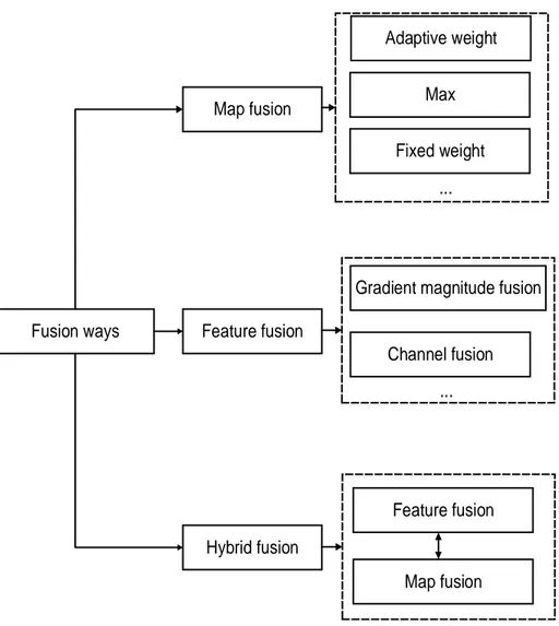
For video SOD, both spatial and temporal information can help the saliency detection. We propose to classify the existing methods into “Map fusion”, “Feature fusion” and “Hybrid fusion” methods. “Map fusion” firstly obtains the spatial saliency map and the temporal saliency map, and then combines them together. “Feature fusion” is to fuse the extracted spatial feature and extracted temporal feature together to give a spatio-temporal feature, which is used to generate the spatio-spatio-temporal saliency map. In order to employ more video saliency information, these two techniques are used together in “Hybrid fusion” recently.

Chapter 2 – Traditional techniques for salient object detection in videos

Video saliency cues

Prior assumption Foreground object Various priors : Saliency measures: Contrast prior Backgroundness prior

Boundary connectivity prior

Moving object

Objectness prior

Distance transform

Matrix decomposition

Graph-based

Markov random field ...

...

2.1. An overview of state-of-the-art methods

Map fusion

Fang et al. [26] give an adaptive weighted fusion rule with an uncertainty computation on both spatial and temporal saliency maps. Kannan et al. [37] propose a Max fusion. For each pixel, the fused saliency is the larger one between spatial saliency and tem-poral saliency. Duan et al. [22] combine these two saliency maps in a non-linear way, based on the assumption that spatially dissimilar and moving blocks are more visu-ally attractive. Tu et al. [81] propose to equvisu-ally weight both saliency maps in a linear way. Zhai et al. [102] propose a dynamic fusion technique where temporal gaze atten-tion is dominate over the spatial domain when large moatten-tion contrast exists, and vice versa. Tu et al. [82] generate two types of saliency maps based on a foreground con-nectivity saliency measure, and exploit an adaptive fusion strategy. Yang et al. [100] propose a confidence-guided energy function to adaptively fuse spatial and temporal saliency maps. Ramadan et al. [71] apply the pattern mining algorithm to recognize spatio-temporal saliency patterns from two saliency maps.

Feature fusion

Wang et al. [89] and Wang et al. [88, 91] detect the salient object from the fused spatio-temporal gradient field. Guo et al. [28] select a set of salient proposals via a ranking strategy. Li et al. [49] fuse the spatial and temporal channel to generate saliency maps, and then use saliency-guided stacked autoencoders to get the final saliency map. Bhattacharya et al. [3] use a weighted sum of the sparse spatio-temporal features. Chen et al. [15] obtain the motion saliency map with spatial cue, then use k-Nearest Neighbors-histogram based filter and Markov random field to eliminate the dynamic backgrounds.

Hybrid fusion

Kim et al. [39] generate the spatio-temporal map based on the theory of random walk with restart, which use the temporal saliency map as the restarting distribution of the random walk. Liu et al. [54] obtain the spatio-temporal saliency map using temporal saliency propagation and spatial propagation. Xi et al. [93] first get spatio-temporal background priors, and the final saliency value is the sum of appearance and motion saliency. Zhou et al. [105] generate the initial saliency map, and propose localized

Chapter 2 – Traditional techniques for salient object detection in videos

estimation to generate the temporal saliency map, and deploy the spatio-temporal re-finement to get the final saliency map, which is then used to update the initial saliency map. Chen et al. [14] get the temporal saliency map to facilitate the color saliency com-putation. Chen et al. [17] detect the motion cues and spatial saliency map to get the motion energy term, which are combined with some constraints and formulated into the optimization framework. Chen et al. [13] employ contrast cue, devise a Markov random field solution and learn multiple nonlinear feature transformations to detect the video salient object detection. Fig. 2.2 shows the classification of the video SOD methods based on fusion ways.

Fusion ways

Map fusion

Feature fusion

Gradient magnitude fusion Max Fixed weight Hybrid fusion Channel fusion ... Feature fusion Map fusion Adaptive weight ...

2.2. Introduction of some existing issues

2.2

Introduction of some existing issues

In this section, a brief overview of some existing issues related to our work is given. The “background prior” [6] is widely used in SOD approaches based on traditional tech-niques. A narrow border of the image is assumed to be the background region. When the salient object pixels appear in the border, their saliency values are set incorrectly to zeros. Besides, video SOD detects the salient object from both spatial domain and temporal domain. How to combine these two saliences together during the detection is complex.

2.2.1

Background prior

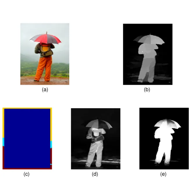
Based on this assumption, the distance transform [72] has been widely used for saliency computation. Traditionally, the distance transforms measure the connectivity of a pixel and the seed set using different path cost functions. Since background regions are as-sumed to be connected to image borders, the border pixels are initialized as the seed set and the distance transform detects a pixel’s saliency by computing the shortest path from the pixel to the seed. The shorter the shortest path is, the higher the saliency is. In the background prior, all the border pixels are regarded as background. Thus, in the distance transform, all the border pixels are set to be seed and their saliency values are thus zeros. This is not true if the object of interest appears in the frame border.

Based on “background prior”, Zhang et al. [103] propose a salient object detection method based on the Minimum barrier distance transform. Combined with the raster scanning, a fast iterative Minimum barrier distance transform algorithm (FastMBD) detects the initial image saliency. In addition, the region possessing a very different appearance from image boundary is highlighted. For each image boundary region, the mean color and the color covariance matrix are calculated using the pixels inside this boundary region. Then the intermediate image boundary contrast map is obtained based on the Mahalanobis distance from the mean color. The final boundary contrast map is got from the four intermediate image boundary contrast maps. After the initial saliency map is integrated with the image boundary contrast map, a morphological smoothing step, a centeredness map and a contrast enhancement operation are used as post-processing operations. Fig. 2.3 gives an example, in which Fig. 2.3 (b) shows the initial saliency result using FastMBD and Fig. 2.3 (c) presents the final result. Fig.

Chapter 2 – Traditional techniques for salient object detection in videos

2.3 (c) is improved but the lower part of the person is not detected, since it touches the border of the frame.

Input

FT

HC

SIA

RC

GS

HS

AMC

SO

GD

MB

MB+

GT

Figure 8: Sample saliency maps of the compared methods. The baseline using the geodesic distance (GD) often produces a

rather fuzzy central area, while our methods based on MBD (MB and MB+) do not suffer from this problem.

5.4. Limitations

A key limitation of the image boundary connectivity cue

is that it cannot handle salient objects that touch the

im-age boundary. In Fig.

9

, we show two typical examples of

this case. Our method MB fails to highlight the salient

re-gions that are connected to the image boundary, because it

basically only depends on the image boundary connectivity

cue. Our extended version MB+, which further leverages

the appearance-based backgroundness prior, can help

alle-viate this issue if the foreground region has a high color

contrast against the image boundary regions (see the top

right image in Fig.

9

). However, when such

background-ness prior does not hold, e.g. in the second test image in

Fig.

9

, MB+ cannot fully highlight the salient region, either.

6. Conclusion

In this paper, we presented FastMBD, a raster scanning

algorithm to approximate the Minimum Barrier Distance

(MBD) transform, which achieves state-of-the-art accuracy

while being about 100X faster than the exact algorithm. A

theoretical error bound result was shown to provide insight

into the good performance of such Dijkstra-like algorithms.

Based on FastMBD, we proposed a fast salient object

de-tection method that runs at about 80 FPS. An extended

ver-Input

MB

MB+

Figure 9: Some failure cases where the salient objects touch

the image boundary.

sion of our method was also provided to further improve the

performance. Evaluation was conducted on four benchmark

datasets. Our method achieves state-of-the-art performance

at a substantially smaller computational cost, and

signifi-cantly outperforms the methods that offer similar speed.

(a)

Input

FT

HC

SIA

RC

GS

HS

AMC

SO

GD

MB

MB+

GT

Figure 8: Sample saliency maps of the compared methods. The baseline using the geodesic distance (GD) often produces a

rather fuzzy central area, while our methods based on MBD (MB and MB+) do not suffer from this problem.

5.4. Limitations

A key limitation of the image boundary connectivity cue

is that it cannot handle salient objects that touch the

im-age boundary. In Fig.

9

, we show two typical examples of

this case. Our method MB fails to highlight the salient

re-gions that are connected to the image boundary, because it

basically only depends on the image boundary connectivity

cue. Our extended version MB+, which further leverages

the appearance-based backgroundness prior, can help

alle-viate this issue if the foreground region has a high color

contrast against the image boundary regions (see the top

right image in Fig.

9

). However, when such

background-ness prior does not hold, e.g. in the second test image in

Fig.

9

, MB+ cannot fully highlight the salient region, either.

6. Conclusion

In this paper, we presented FastMBD, a raster scanning

algorithm to approximate the Minimum Barrier Distance

(MBD) transform, which achieves state-of-the-art accuracy

while being about 100X faster than the exact algorithm. A

theoretical error bound result was shown to provide insight

into the good performance of such Dijkstra-like algorithms.

Based on FastMBD, we proposed a fast salient object

de-tection method that runs at about 80 FPS. An extended

ver-Input

MB

MB+

Figure 9: Some failure cases where the salient objects touch

the image boundary.

sion of our method was also provided to further improve the

performance. Evaluation was conducted on four benchmark

datasets. Our method achieves state-of-the-art performance

at a substantially smaller computational cost, and

signifi-cantly outperforms the methods that offer similar speed.

(b)

Input

FT

HC

SIA

RC

GS

HS

AMC

SO

GD

MB

MB+

GT

Figure 8: Sample saliency maps of the compared methods. The baseline using the geodesic distance (GD) often produces a

rather fuzzy central area, while our methods based on MBD (MB and MB+) do not suffer from this problem.

5.4. Limitations

A key limitation of the image boundary connectivity cue

is that it cannot handle salient objects that touch the

im-age boundary. In Fig.

9

, we show two typical examples of

this case. Our method MB fails to highlight the salient

re-gions that are connected to the image boundary, because it

basically only depends on the image boundary connectivity

cue. Our extended version MB+, which further leverages

the appearance-based backgroundness prior, can help

alle-viate this issue if the foreground region has a high color

contrast against the image boundary regions (see the top

right image in Fig.

9

). However, when such

background-ness prior does not hold, e.g. in the second test image in

Fig.

9

, MB+ cannot fully highlight the salient region, either.

6. Conclusion

In this paper, we presented FastMBD, a raster scanning

algorithm to approximate the Minimum Barrier Distance

(MBD) transform, which achieves state-of-the-art accuracy

while being about 100X faster than the exact algorithm. A

theoretical error bound result was shown to provide insight

into the good performance of such Dijkstra-like algorithms.

Based on FastMBD, we proposed a fast salient object

de-tection method that runs at about 80 FPS. An extended

ver-Input

MB

MB+

Figure 9: Some failure cases where the salient objects touch

the image boundary.

sion of our method was also provided to further improve the

performance. Evaluation was conducted on four benchmark

datasets. Our method achieves state-of-the-art performance

at a substantially smaller computational cost, and

signifi-cantly outperforms the methods that offer similar speed.

(c)

Figure 2.3: FastMBD15 [103]. (a) Input image, (b) Minimum barrier distance transform with the Raster Scan, (c) Final result. (Figures are copied from the published paper [103])

Tu et al. [80] combine the Minimum barrier distance transform with a minimum span-ning tree. Instead of finding the shortest distance, they search the shortest path in the minimum spanning tree. The minimum spanning tree is constructed by avoiding edges with large color difference between adjacent pixels. To ensure the detection of the salient object that touches the frame border, the boundary color dissimilarity measure is used. They first divide the boundary into three groups according to their color values and then the intermediate pixel-wise color dissimilarity map of each group is calculated using the Mahalanobis distance. The final color dissimilarity map is the weighed sum of three intermediate color dissimilarity maps. In the post-processing, a boundary dissim-ilarity map, a pixel location dependent masking and an adaptive contrast enhancement are used. Fig. 2.4 gives an example to show the intermediate results.

Jiang et al. [36] propose a saliency detection via absorbing Markov chain on an image graph model. It measures image saliency by using the similarity of the absorbed time of each transient node with the background absorbing nodes (the image border). It considers both the edge weights on the path and the spatial distance when comput-ing the absorbed time, so the object that is different from or far from the background absorbing nodes can be highlighted. The homogeneous background region in the im-age center may not be effectively suppressed. The saliency map is updated using a weighted absorbed time. Fig. 2.5 compares the results without update processing and