HAL Id: hal-00861063
https://hal.archives-ouvertes.fr/hal-00861063
Submitted on 11 Sep 2013HAL is a multi-disciplinary open access
archive for the deposit and dissemination of sci-entific research documents, whether they are pub-lished or not. The documents may come from
L’archive ouverte pluridisciplinaire HAL, est destinée au dépôt et à la diffusion de documents scientifiques de niveau recherche, publiés ou non, émanant des établissements d’enseignement et de
From Recurrent Neural Network to Long Short Term
Memory Architecture
Xiaoxin Wei
To cite this version:
Xiaoxin Wei. From Recurrent Neural Network to Long Short Term Memory Architecture. 2013. �hal-00861063�
University De Nantes
Master Multimedia
and Data Management(MDM)
From Recurrent
Neural Network to Long Short Term
Memory Architecture
Application to Handwriting Recognition
Author:
supervisor:
Xiaoxin WEI Christian VIARD-GAUDIN
Harold MOUCHERE
Abstract
Despite more than 30 years of handwriting recognition research, Recognizing the unconstrained sequence is still a challenge task. The difficulty of segmenting cursive script has led to the low recognition rate.
Hidden Markov Models (HMMs) are considered as state-of-the-art methods for performing non-constrained handwriting recognition. However, HMMs have several well-known drawbacks. One of these is that they assume the probability of each observation depends only on the current state, which makes contextual effects difficult to model. Another is that HMMs are generative, while discriminative models generally give better performance in labelling and classification tasks. Recurrent neural networks (RNNs) do not suffer from these limita-tions, and would therefore seem a promising alternative to HMMs. A novel type of recurrent neural network, termed as Bidirectional Long Short-Term Memory (BLSTM) architecture, will be studied in this thesis. A sequence concatenating technique called Connecionist Temporal Classification (CTC) is applied. Finally, Three extended decoding algorithm: Levenshtein Distance(LD), full path(FD), max path(MD) are proposed insighted by HMM to have a lexicon-based classification. The system BLSTM-CTC-FP is demonstrated to be robust to lexicon-based recognition and reduce 50% error than the ex-isting best model.
Keywords Handwriting recognition, Sequence modeling, Neural network, Long short term memory, Lexicon-based.
Contents
Abstract 1
1 Introduction 4
1.1 Background . . . 4
1.2 Scope and objective . . . 5
1.3 Thesis Layout . . . 6
2 State of art 7 2.1 Overview . . . 7
2.2 Explicit Segment System . . . 8
2.2.1 Segmentation . . . 8
2.2.2 Character-base Classifier . . . 11
2.3 Implicit Segment . . . 12
2.3.1 Generative Model . . . 12
2.3.2 Hybrid of Generative and Discriminative Model . . . . 16
2.3.3 Discriminative Model . . . 19
2.4 Summary . . . 20
3 Long Short Term Memory 22 3.1 Overview . . . 22
3.2 LSTM architecture evolution . . . 22
3.2.1 Input and Output Gate . . . 23
3.2.2 Forget Gate activation: button to forget . . . 24
3.2.3 Peephole Connection: immediate supervisor . . . 25
3.3 Topology . . . 27
3.4 Backprobagation through Time: learning weights . . . 28
3.5 Bi-direction Extension: BLSTM . . . 29
3.6 Summary . . . 30
4 Connectionist Temporal Classification 31 4.1 Overview . . . 31
4.2 From Timestep Error to Sequence Error . . . 31
4.3 Sequence Objective Function . . . 35
4.4 Decoding . . . 36
4.4.1 Levenshtein Distance (LD) . . . 37
4.4.2 Full Path Decoding (FP) . . . 38
4.4.3 Max Path Decoding (MP) . . . 39
5 Experiment 40 5.1 Overview . . . 40 5.2 IRONOFF Dataset . . . 40 5.3 Framewise Recognition . . . 41 5.4 Temporal Recognition . . . 43 6 Conclusion 49 Reference 50
1
Introduction
1.1
Background
Handwriting is a skill that is personal to individuals. Fundamental char-acteristics of handwriting are three folds. It consists of artificial graphical marks on a surface; its purpose is to communicate something; this purpose is achieved by virtue of the mark’s conventional relation to language. Writing is considered to have made possible much of culture and civilization. Hand-writing recognition is the task of transforming a language represented in the spatial form of graphical marks into its symbolic representation.
Handwriting is still one of the most important communication methods even effected by the widespread acceptance of digital computers nowadays. For example, people are still requested to signed personally on documents instead of printed ones. Besides, a pen-based interfaces in digital devices are popular in the recent decades and will play a more important role in the future due to its natural interaction way for human and machine.
Therefore, Some tasks have been put forward to understand the hand-writing recognition by computers [26] ,which includes handhand-writing
recogni-tion, interpolation and identification. Handwriting Recognition is the task of
transforming a language represented in its spatial form of graphical marks into its symbolic representation. Handwriting interpretation is the task of de-termining the meaning of a body of handwriting, e.g, a handwritten address. Finally Handwriting Identification is the task of determining the author of a sample of handwriting from a set of writers, like signature verification.
On the other side, according the input data, Handwriting can be casted into online and offline data. In the online case, the two-dimensional coordin-ates of successive points of the writing as a function of time are stored in order. In offline case, only the completed writing is available as an 2-D image. To some extent, Handwriting Recognition is the basis to the other two tasks. Although there are many existing application, the technology is not fully matured. Thus the main contribution of this thesis will focus on hand-writing recognition and only the online data is considered.
Figure 1: different kinds of handwriting sequence data input.Line 1 is box handwriting which the position of each letter is known; Line 2 is script hand-writing in which each letter is isolated. Line 3 is natural handhand-writing which maybe cursive and unconstrained
1.2
Scope and objective
There are still two kinds of different tasks in Handwriting Recognition, which is to recognized isolated character and sequence. Unsurprisingly, the latter on is more difficult. Isolated character recognition has been achieved a good performance, about 99% percent for different language [34] [11] [9]
For sequence Recognition, There are different kinds of sequence input data depending on whether the position of each letter in the stream of se-quence has been defined. In the first situation of Figure 1, the writer is forced to write each letter into a box, which the position is known. Also, the writer can be asked to write each letter separately. In this case, each letter will be isolated. the position is unknown but easy to obtain by applying some con-ditional cuts. The previous two situations can be called constrained writing because the writers writes according to some constraints. However, this does not happen in humans actual writing habits, which usually is cursive and unconstrained. Just like in the third line of the figure, each letter in a word is unknown and difficult to achieve. Therefore, it is still challenge to develop a robust and reliable system for that kind of sequence.
The main contribution of this thesis are as follows:
a). analyze the existing related sequence recognition system, point out the limitation and the relationship between BLSTM-CTC
b). apply the BLSTM-CTC system to different handwriting recognition c). explore the optimal features for Long Short Term Memory(BLSTM) d). extend the CTC technique to lexicon-based decoding using various
method.
e). comparison of lexicon based BLSTM-CTC with state of art models, like hybrid of HMM and NN.
1.3
Thesis Layout
The first section presents some background, the issue related to handwriting recognition and the scope, aim and contribution of this thesis. The rest of the thesis is organized as followed: Chapter 2 presents the state of the art of handwriting sequence recognition, which has been categorized into two taxonomy: implicit and explicit segment systems. Both will be listed the main technique and related papers. The purpose of this section is trying to link and distinguish the BLSTM-CTC with other systems.
In section 3, theoretical foundation of Long Short Term Memory (BLSTM). LSTM is a multi-active recurrent neural network with a more sophisticated hidden neuron called memory block. The topology of LSTM and its learning algorithm Back propagation through time (BPTT) are also referred. Finally, a forward and backward pass recurrent structure is applied to equip with bidirection.
A word level concatenating technique is discussed in section 4, called Connectionist Temporal Classification(CTC),which is used to transcribe the character-based BLSTM error onto sequence error. It is actually a HMM termilogy take advantage of some algorithm, like forward and backward, Vi-terbi. Thanks to HMM, different decoding methods is proposed to transplant on CTC in lexicon-based recognition.
Experiments are conducted in section 5 including framewise and temporal sequence task. Lexicon-based evaluation is used to compared with some state-of-art model.
2
State of art
2.1
Overview
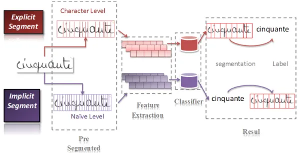
The sequence recognition models can be casted into two category: explicit segment and implicit segment. The overview of these two systems can be seen in Figure 2. Both includes pre-process(here we just point out segment), feature extraction, classifier and then get the final result(segments and se-quence label). There are two main distinction points between implicit and explicit, The first system needs dedicated cutting technique to be cut seen like character. By contrast, the segment of second system is based on heur-istics information. Secondly.In the explicit, we can not get the result unless we know the segment, but the implicit segment system is the opposite, which it first get the result then segments.
Figure 2: Sequence Recognition System Taxonomy 1.Explicit Segment
The recognition task of constrained handwriting sequence is similar to isolated character recognition as we can achieve the segmentation of the se-quence. Then a sequence level can be concatenating with characters. How-ever, to recognize the unconstrained sequence data is much more complicated since the segmentation information is unknown. One approach is to recognize individual characters and map them onto complete words, which is the same
as the previous case. This needs to first classify each segment. However, seg-mentation is difficult for cursive or unconstrained text, at least as difficult as to recognize. In this case, if the segmentation is not reliable, the recognition will be even harder. On the other hand, segmentation is not finally defined unless the words has been recognized. This will create a circular dependency between segmentation and recognition referred to as Sayre’s paradox [12]. 2.Implicit Segment
Another approach to the unconstrained sequence is to simply ignore the Sayre’s paradox, and carry out segmentation without "much effort",just seg-ment them into basic strokes, slices or points, rather than characters. this will be much easier. for example, for online data, the stroke boundaries can be defined as the minimum of the velocity. For offline data, we can cut each sequence at the minimum vertical histogram. The segmentation and recogni-tion is usually at the same. The final segmentarecogni-tion can not be defined unless the recognition result is known.
This Chapter has been put forward the taxonomy of sequence recognition system in Section 1. The overview of explicit segment system will be in Section 2, including the segment technique and classifiers. Section 3 will describe implicit system. Section 4 comes to the conclusion.
2.2
Explicit Segment System
For the explicit segment sequence recognition system, there are usually four steps: pre-process, segmentation,feature extraction, classifier.There are some common operations in sequence preprocessing, like noise removal, slant angle correction, smoothing, which will be the same to the implicit Segment Sys-tem.
2.2.1 Segmentation
Character segment is crucial to the following step classifier in this kind of recognition system. if the segments is not correct, the result will be wrong no matter how robust the classifier is. Then researchers spend no effort to improve the performance of character segmentation. Some segmentation techniques [10] is listed as followed:
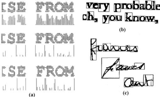
Dissection is applied for many years, like projection analysis, connected component processing, and contextual post processing grapheme. more in-formation of these methods is shown in the figure 3.
Space and Pitch: In machine printing, vertical whitespace often serves
to separate successive characters. This property can be extended to hand-printed by providing separated boxes in which to print individual symbols. The notion of detecting the vertical white space between successive charac-ters has naturally been an important concept in dissecting images of machine print or handprinted.
Projection: projection is shown in Figure Figure 3(a), vertical
projec-tion is applied in the offline handwriting image. It is an easy matter to detect white columns between characters. but it fails to make the character O-M separation. Line 2 in (a) apply the differencing measure for column splitting and it will give a clear peak at the separated point. However, O-M case still fails. Line 3 in (b) difference after column ANDing. The image transformed by an AND of adjacent columns, which leads a better peak in between O-M.
Connect Component Analysis: Figure 3 (b) shows how connected
component works. The example illustrates characters that consists of two components or more than one components will have wrong segments.
Grapheme: in Figure 3 (c), Here, a Markov model is postulated to
rep-resent splitting and merging as well as misclassification in a recognition pro-cess. The system seeks to correct such errors by minimizing an edit distance between recognition output and words in a given lexicon. An alternative ap-proach still based on dissection is to divide the input image into sub-images that are not necessarily individual characters. The dissection is performed at stable image features that may occur within or between characters.as for example, a sharp downward indentation can occur in the center of an ’M’ or at the connection of two touching characters.
2.Ligatures and Concavity
Dissection is not efficient for cursive handwriting script. Other improving features like ligatures and concavities [22] are also used for cutting point.Marks an x-coordinates as a ligatures point where the distance between y-coordinates of the upper half and lower half of the outer contour for a x-coordinate is less than or equal to the average stroke width. Besides, concavity features in the upper contour and convexities in the lower contour are used in conjunction with ligatures. The process is in following Figure 4.
Figure 3: Dissection technique. (a)Line 1: vertical projection; Line 2: differ-ence of vertical projection; Line 3: differencing measure of ANDing column; (b)connected component Analysis; (c)Grapheme
Figure 4: Segmentation of cursive script by ligature feature (a) Ori-ginal test image. (b) slant normalization.(c) Splitting upper and lower contours.(c)Ligatures based on the average stroke width.(e) Concavit-ies/convexities.(f)Segmentation points.
3.Over Segment
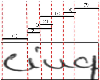
However, the segments result is still unreliable without considering the recognition feedback. Therefore a more modern way is a hybrid of segment and recognition. A dissection algorithm is applied to the image, but the in-tent is to "over-segment", i.e, to cut the sequence in sufficiently many places that the correct segmentation boundaries are included among the cuts made, as in Figure 5.
Once this is assured, the optimal segmentation is defined by a subset of the cuts made and the classification is brought to choose the most promising segmentation. The strategy is in two steps. In the first step, a set of likely cutting paths is determined, and the input image is divided into elementary components by separating along each path. In the second steps, segmentation hypotheses are generated by forming combinations of the components. All combinations meeting certain acceptability constraints(such as size, position, etc.) are produced and scored by classification confidence. An optimization algorithm is typically implemented on dynamic programming principle. One example is shown in figure 5
Figure 5: Over segment strategy. There are seven sub paths, and the optim-ized combination path is 1-2-5-7.
2.2.2 Character-base Classifier
After the segmentation, we assume the result is character-based, as the clas-sifier and segmentation is independent, various character-based clasclas-sifier can
be chosen, like HMM(hidden Markov model) [25], neural network [34], sup-port vector machine(SVM)[4].
2.3
Implicit Segment
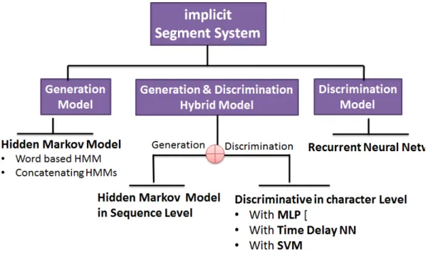
Implicit Segment System is quite different from the previous one. It is not possible to surely say what common procedures they need. Since segmenta-tion and recognisegmenta-tion don’t separate so clearly, and some models even don’t need a segments. But we can cast them into three catalogs according to the types of the classifier in Figure 6. These are generative, discriminative, and the hybrid of both. Each of them will be discussed in this section.
Figure 6: Implicit Segment Sequence Recognition System Taxonomy
2.3.1 Generative Model
The most famous generative model dealing with sequential data is hidden Markov model(HMM). before starting, this subsection first go through some basic theory which is also related to the technique of the thesis main word in later section, and then the model applied HMM to handwriting sequence recognition.
HMM [5] is a statistical model of Markov process, which succeeds to treat with sequential data by observations and underlying states. The Markov hy-potheses define that the probabilistic description is truncated to just the current state and the predecessor state, Also, the observation is not determ-inistic which depend on the current state. Each HMM is represented by a set of parameter λ = (A, B, π), where A denotes the transition matrix, B the matrix of emission, and π the initial state distribution. With an HMM, the first stochastic process is represented by the probability that the HMM generated observations and second by the sequence of state transitions un-dertaken. There are two basic types of HMM: discrete and continuous. In the case of discrete HMM, the matrix B contains discrete probabilities to each observation while in continuous, B is not directly a matrix, but represents mixtures of Gaussian or other PDFs.
There are three algorithms that are respective related to three main issues of HMM.
Forward and Backward Algorithm
One the main issue of HMM is recognition. Given several HMMs models
λi, recognition is to classify the model with most probabilities that a given
string belong tol. This is to calculate argmaxiP (O|λi). The problem is to
sum up all the paths of states that equal to the given observation, which is a time-consuming work. Forward and backward algorithm is generated to calculate this sum value efficiently. Since we can compare this with LSTM forward and backward algorithm in later section, we go a little further about it.
The main idea of the algorithm is to compute a forward variable αt
iand
backward variable βt
i, in which αti denotes the probability of all the paths
equal to the partial observation ending at time t with state i and meanwhile βt
i denotes the probability of all the paths equal to given observation starting
a time t with state i. Assume there are N states, T time length, then the probability of a given HMM model of an observation can be translated to.
P (O|λ) = N X i=1 ( N X j=1 (αtiaijbtj + 1βjt+ 1)) = N X i=1 (αtiβit) (1)
Forward and backward variable is like the ’save points’ in the paths. It is not able to retrieve the probability of each path through this algorithm. But it doesn’t matter since we only need the final sum probability, which can be
achieved by adding the ’save points’. Viterbi Algorithm
Another issue of HMM is decoding. Given a string of observation and a model λ, how to extract the optimal underlying states path. We can also compare it with the later proposed CTC decoding issue in Section It is sim-ilar to the forward and backward algorithm. We have the ’save points’ of
each sub path call δt
i. The differences to αti and βit is δit is not a sum value
but maximum. It denotes maximum probability path ending at time t of state i among all the partial paths. Finally, the optimal state path can be obtained by traced back from time T to time 1 by choose the state with max
δit at each time t. Since the it is proposed by A.Viterbi [3], the algorithm is
called Viterbi .
Baum-Welch Algorithm
The training problem is crucial since a optimized model is basic guar-antee to recognition and decoding. However, there is no known analytical solution that exists for the learning problem. The popular solution is iter-ative algorithm: Baum-Welch algorithm [2]. It is a generalized expectation-maximization(EM) algorithm for finding maximum likelihood estimates and posterior mode estimates for the parameters.
The algorithm perform alternatively between E step and M step. In E step, it calculate an expected count of the particular transition-observation pair while in M step, we update the parameters by maximizing the expected likelihood found on the E step. The parameters found on the M step are then used to begin another E step.
HMM is first distinguished itself by speech sequence processing and re-cognition. on-line handwriting is very similar to the problem of continuously speech recognition. Online handwriting can be viewed as a signal (x,y) over time, just like in speech. Then more and more researchers started to extend HMM to handwriting recognition. The work includes [32] [16] [7] [19] [37] [36]apply HMM in cursive handwriting recognition.
A classic application is handwriting word recognition using word-level HMM framework [7].The meaning of word-level is that each word in the
dictionary forms an HMM λi, the recognition is performed by presenting
the observations to all HMMs and select the model with greatest
probabil-ity P (O|λi) using forward and backward algorithm. Usually, it is a holistic
method, segmentation is not necessary. All the classifier knows is the whole word, but it can’t define which characters it contains. Therefore, we only can classify the exact word that occurs in the training set.The problem is that we have millions of words although we can have a small and limited alphabet(26 for English lowercase, and 65 for French). It is impossible to model all the word as an HMM and it will cost time for recognizing. Therefore this is always limited to small lexicon size.
The most common solution is to model each character in the alphabet as an HMM then concatenating them as a word. [32] developed a two-level based HMMs for online cursive handwriting recognition: letter-level and word level. The input data is sampling points, each of them first are represented by 6 features(x,y,δx,δy, penup/pendown, x − max(x)) then clustered into 64 centers. There is no segments needed and each point finally describe into 64 discrete value. 53 HMMs with 7-states left-right topology are formed to rep-resent a single symbol including 52 character and one for white space.Since the penning of a script often differs depending on the letters written before and after, additional HMMs are used to model these contextual information. [19] uses the similar structure for offline cursive handwriting . The se-quence data first are segmented into letters or pseudo letters by ligature fea-tures. The letters or pseudo letters are described by some histogram feature, which need to be tantalized. For training, Each symbol HMM is discrete and characterized by a more delicates topology which takes the under-segments, over-segments and null value into consideration. The word model is made up by concatenation of appropriate letter models consisting of elementary HMM. The Viterbi algorithm is used in recognizing the letters in a word.
Compared with the previous discrete HMM, [37] apply a continuous dens-ity two-level continuous HMM for offline data. The segment is replaced by cutting the image into overlapping sliding windows, which are extracted pixel-based low level feature. Letter-based HMMs are generated by assuming the features in Gaussian mixture distribution.
In conclusion, there are some commons in word-level and concatenating HMMs. First, compared with the previous explicit segment system, the seg-ment in HMMs is easier or even not necessary. Besides, the segseg-ment does
not take all the risk as HMM have a hidden states. Second, both word-level and concatenating HMMs directly recognize the result word without knowing each observation belong to which letter in the word. It means that we get the result even not awaring the segments. The segments can then be retrieved by the Viterbi algorithm, which is quite different to explicit segment system. On the other hand, the above HMM models suffer from some drawbacks. First, word-level HMM is limited to small lexicon size while in two-level HMMs, it is difficult to train the letter-base HMMs since the train data-sets usually don’t provided the segments. Either the system can segment sequence data into letter by hand or use another isolated character dataset. The latter lose the contextual information while the former is time consum-ing and not practical when the amount is large. Secondly, considerconsum-ing the a handwriting recognition system , where each HMM represents a letter, the HMM corresponding to a given letter only train by the samples of this let-ter. So an given symbol HMM neither takes the number of classes nor the similar symbol into account. Its generative capability does not maximize the distance between classes. Thirdly, both HMMs model are subjected to some assumption which may be restrict in practice. In discrete model, The features will lose information after quantizing. However, continuous model still suffers by assuming several Gaussian mixture model.
2.3.2 Hybrid of Generative and Discriminative Model
Given the drawbacks of HMM, the reason is mainly due to its arbitrary parametric assumption that given the estimation of a generative model from data. However, it is well known that for classification problems, instead of constructing a model independently for each class, a discriminative approach should be used to optimize the separation of classes.
As a consequence, by combining HMMs and discriminative model, such as neural network(NN) it is expected to take advantage of both. The researchers has explored to apply different kinds of NN associated with HMM to boost the performance of handwriting recognition. such as MLP, TDNN,RNN.
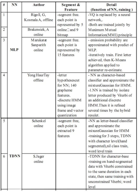
Table 1: state-of-art model:HMM Hybrid with different kinds of Neural Net-work applied to Handwriting recognition
However, Neither the structure of how to combine NN and HMM nor how to train them is surely final defined. Thus the optimal hybrid modeling with NN and HMM is still an open question. Some related work is shown in the following Table 1
In the initial combination paper No.1 and 2 in Table 1 [28] [8], VQ in a discrete HMM is realized by replacing the usual k-means VQ by a neural network. It allows to eliminate the quantization error. Maximize the MMI principle of HMM enables to backprobagate the error to train the neural network. Paper No.3 [24] is a similar case but apply to continuous HMM, where the emission probability is approximated with predict of NN.
Although the early system contain neural network, but it is not able to involve much discriminative information. Paper No.4 in Table 1 [33] is a breakthrough in the merge of NN and HMM. NN is the character-based classifier. The isolated training data is extracted by Viterbi from baseline recognizer. The output of NN divided by the letter class prior are used dir-ectly as observation probability for the letter-level HMM. A ligature HMM and word HMMs are also designed in the system. The training process can be iterated by using the segment from the hybrid model.
The function of NN in Paper No.5 in Table 1 [29] is same to No.4[33] as approximate the Gaussian density function.
Paper No.5 [31] describe a similar structure as Paper No.4, where the mixture Gaussian is replaced by outputs of NN divided by the probability class except RNN is able to memorize and each output node of RNN is linked to just one state of a HMM. The problem is the amount of training data re-quired for neural nets, which can be higher than for pure HMM system.
2.3.3 Discriminative Model
Although the NN-HMM hybrid well outperforms the HMMs model, it’s still in the generation loop and constrained by distribution assumption. Discrim-inative models doesn’t suffer from this problem. However, it is difficult to design a sequence recognition model only with discriminative model since it lack the ability to handle time varying sequences.
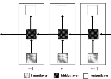
Recurrent Neural Networks are a particular category of ANNs, which is capable of storing memories and dynamically driven compared with other feedforward NN like MLP. There are various topology of RNN, one classic example is that there is one hidden layer. All the inputs are connected to hidden layer which is fully connected to itself. The recurrent link is actually a time delay connection, which if unfolded can be drawn as in Figure 7. The weights learning always use the algorithm of backpropagation through time.
Figure 7: Classic Recurrent Neural Network
But at the same time, RNN has its own problem when applied to hand-writing recognition:
the current architecture fails to have long term memory. The reason is that the influence of a given input on the hidden layer, and therefore on the network output, either decays or blows up exponentially as it cycles around the network’s recurrent connection. This shortcoming is called
[6] which point out that it is hard for RNN to bridge gaps of more than 10 time steps between relevant input and target events, which is obviously unpractical for handwriting sequence.
The traditional RNN can not be directly used to sequence labeling since the objective function is unable to concatenating the sequence error.
A.Gers has solved the above problems. The gradient vanish problem is solved a multi-active structure of RNN called Long Short Term Memory (LSTM) [13] , while a HMM terminology objective function [15] is generated to deal with the second problem. Both techniques will be illustrated in the following section and will be the main work of this thesis.
2.4
Summary
This section first introduces the taxonomy of handwriting sequence recogni-tion system, which is explicit and implicit segment. In the explicit system, the sequence recognition is obtained after the segment is decided, while we directly get the recognition result in implicit model, which can then be used to achieve the segment. Besides, the state-of-art of handwriting recognition system is then listed to further their feature and own problem. For expli-cit segment model, it suffers in the ambiguity and unreliability of segment process. On the other hand, implicit model is outperformed in generative classifier and the hybrid of generative and discriminative. However, the ex-isting models are limited by the HMM generation condition.
The sequence recognition model BLSTM-CTC is similar to the previous discussed HMM-NN hybrid except it is fully discriminative. Like the hybrid, an NN structure is used for character-based discrimination, which is role of BLSTM. Besides, in the hybrid, HMM is responsible for sequence concaten-ating while in BLSTM-CTC, it use some forward backward algorithm and HMM idea to translate the sequence error into LSTM model. All will be detailed discussed in the later section.
But here we can first forecast the superiority compared with the previous HMM-NN hybrid models. First, the character-based discriminative classifier is trained by the data which is exactly sequence data containing contextual information without hand segment or isolation procedure. Second, character-based classifier can also fulfill the word-level recognition by a concatenating objective function. All is due to the main difference between BLSTM-CTC
3
Long Short Term Memory
3.1
Overview
As discussed in previous section, recurrent neural networks is able to deal with sequence data by storing variant time series, However, it fails to have long term memory.In this section, a discriminative model called Long Short Term Memory will be discussed, which is capable to deal with long time se-quence. LSTM was first introduced by Sepp Hochreiter [17], The main idea of LSTM is to design a constant error cell by multi-active hidden neurons. The structure of the neurons has been modified over ten years to have better performance.
The rest context will be organized as followed: The evolution of LSTM structure is shown in Section 1, which includes input, output, forget gate and peephole connection. After defined the neurons, Section 2 describe different topology. A directional technique is added in section 3 along with the al-gorithm. Section 4 describe the learning algorithm needed: backprobagation through time(BPTT). Summary is given in Section 5.
3.2
LSTM architecture evolution
This subsection will be illustrated evolution of multi-active unit used in LSTM. First we define some annotation as followed:
- Subscription wjj0 is from unit j to j’. As traditional classic RNN
archi-tecture, there are input layer, recurrent layers and output layer. The hidden layer is constructed by hidden neuron, which is called memory block(MB). One memory block can contain one or several memory cell(MC). For annota-tion of the nodes, i denotes the unit index in the input layer. Greek letter
ρ, π, φ is the subscription of input gate, output gate, and forget gate in the
recurrent layer. c refer to one of the cells in a block. st
c is the state of cell
c at time t. Note that only the cell output connected to other block in the
hidden layer, other LSTM activation like state is only visible in the block. We use h to refer to the cell output from other blocks in the hidden layer.
- Inputs and Outputs of Units: trigger to read and write xtj is the
network input to any unit j at time t. For example xt
i is the network input
from unit i in the input layer at time t. yt
j is value of xtj after activation.
For example, any cell output unit after activation at time t in a block can
be expressed as yt
activation function of cell input and output respectively.
- Units Number Let I be the number of nodes in input layer, K be
the size of output layer and H be the number of cells in the hidden layer. C denotes the number of memory cells in one block.
3.2.1 Input and Output Gate
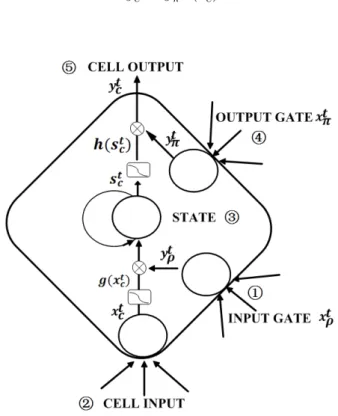
Memory cell was introduced by J.Schmidhuber [6] to have a constant error flow. The main idea is that as time goes, the NN is able to protect stored information from perturbation while outputs also require protection against perturbation. Therefore an input and output gate is generated in the memory cell, where input is the switch of reading while output is the trigger to writer. The cell in the hidden layer is not able to receive the information to store unless the input gate is open. Also, only when the output gate is open, can the cell emits the store information to output layer or to recurrent link.
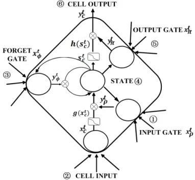
Thus, Memory cell is actually a multi-active neurons with input and output gate activation. The architecture of memory cell is shown in Figure 8 The equation is shown as followed:
Input Gates : xtρ= I X i=1 wiρxti | {z }
f rom input layer
+ H X h=1 whρyt−1h | {z } f rom recurrent (2) ytρ= f (xtρ) (3) Cells : xtc = I X i=1 wicxti + H X h=1 whcyt−1h (4) stc= st−1c |{z} previous state + ytρg(xtc) | {z } current state× input gate (5) Outputs Gates : xtπ = I X i=1 wiπxti | {z }
f rom input layer
+ H X h=1 whπyht | {z } f rom recurrent (6)
Cell Outputs :
yct = ytπh(stc) (7)
Figure 8: LSTM memory block with one cell, containing input gate and output gate. The self-recurrent(with weight 1.0) indicates feedback with a delay of one time step.There are two operation: a squarish activation and a multiplier. The number shows the updating steps.
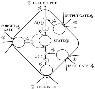
3.2.2 Forget Gate activation: button to forget
The original LSTM allows information to be stored across arbitrary time lag, and error signals to be carried far back in time. However, if we present a continuous input stream, the cell states may grow in unbounded fashion. It is also not practical since we need to reset the cell states occasionally in the real task, e.g, at the beginning of a new character sequence.
Thus, an adaptive forget gate is added [14]. which is the same to previous LSTM except the accumulate states not adding the previous directly but with some adjustment. Architecture can be seen as Figure 9
Figure 9: LSTM memory block with one cell,adding forget gate, which is an adjustment to the previous stat. The number indicates the updating order.
The forget gate is defined as same as input and output gate, and calcu-lated before cell state.
F orget Gates : xtφ = I X i=1 wiφxti + H X h=1 whφyht−1 (8) ytφ= f (xtφ) (9) Cells states : stc= btφst−1c | {z } previous state adjustment + ytρg(xtc) | {z } current state× input gate (10)
3.2.3 Peephole Connection: immediate supervisor
LSTM is equipped with long short term memory and able to reset, but how do it know how long of memory the model needs. For example, when output
gate is close, each gate receive none from the cell output. The solution is to allow all gates to inspect the current cell state even when the output gate is closed. The adding connection is called "peephole" [13], which can be founded in Figure 10
Figure 10: LSTM memory block with " peephole" connection, with which all the gates can supervise the cell state.
So state function stay the same, while each gate function modified: Input Gates : xtρ= I X i=1 wiρxti | {z }
f rom input layer
+ H X h=1 whρyht−1 | {z } f rom recurrent + C X c=1 wcρst−1c | {z } f rom cell;state (11) ytρ= f (xtρ) (12) F orget Gate : xtφ= I X i=1 wiφxti+ H X h=1 whφyt−1h + C X c=1 wcφst−1c (13) ytφ= f (xtφ) (14)
State function is calculated as , Noting that the input and output gate is related to previous t − 1 state, output gate is refer to current t state:
OutputsGate : xtπ = I X i=1 wiπxti+ H X h=1 whπyht + C X c=1 wcπstc (15) ytπ = f (xtπ) (16)
3.3
Topology
After clearly discussing the architecture of memory block in LSTM, which includes an input gate, output gate and forget gate along with peephole con-nection. The next step is to define the whole neural network layout.
In terms to application, the more difficult the task is, more dense and complicated connection is needed. for example, we can:
1. Increase the cell number in a block. 2. Increase recurrent neurons.
3. Direct shortcut from input layer to output layer.
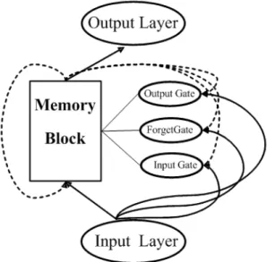
But more dense the network connection is, more time will be needed for training and testing.For experiments proves that one cell in a block is suffi-cient to handwriting recognition. Thus a not so dense topology is introduced and applied to the experiment in Chapter 5.The topology is shown in Fig-ure 11, in which input layer is all connected to the hidden layer(gates and cell inputs). Besides, The cell outputs are fully time delay recurrent to the hidden layer and feedforward to the output layer. There is only one cell in the hidden layer constrained by the figure size. In hidden layer, more cells added will increase the input stream to cell inputs and gates.
Here supposed a classification task with output layer size O. input layer size I. We can set block size in hidden layer to H, There are C cells in one block, which share the same input, forget and output gate. The total number weights can be added by the following three items:
F rom Input Layer :
I × H × C | {z } T o Cell Input + 3 × I × H | {z } T o Gates (17)
Figure 11: LSTM topology with one single-cell block in the hidden layer. The solid line indicates the feedforward connection(from input layer & to output layer), and the shade line refers to the recurrent link from cell output.noting that the peephole connection is not drawn in the figure due to the size limits.
F rom Output Layer :
O × H × C
| {z }
F rom Cell Output
(18) F rom Recurrent : (H × C) × (H × C) | {z } T o Cell Output + (H × C) × (3 × H) | {z } T o Block Gates + 3 × H | {z } P eephole Connection (19)
3.4
Backprobagation through Time: learning weights
Backpropagation is the most widely used tool in the field of artificial neural networks. The Basic backpropagation has been well applied to feedforward neural network. Its further extension, called backpropagation through time (BPTT) was first introduced in [20] , which can deal with dynamic system like recurrent neural network.
Here is the BPTT algorithm pseudo-code applied to LSTM can be de-tailed seen in [13].
3.5
Bi-direction Extension: BLSTM
The previous LSTM with input, forget and output gate is capability with long time lag, state reset and resolve temporal distance. But all states are accumulated forward. In real task, the system is usually requested to take backward information into consideration. For example, the cursive handwrit-ing script is one character connected with another, Thus the character after is as important as the character before.
[30] proposed a bi-directed RNN structure to overcome the limitation of single direction. The idea is to split the state neurons of a regular RNN in a part that is responsible for positive time direction(forward states) and the negative direction(backward states). Outputs from forward states is not con-nected to backward states. This is like two separate hidden layer which both linked from input layer and meets at output layer. The unfolded topology is shown in figure 12.
Figure 12: General structure of the bidirectional recurrent neural network shown unfolded in time for three time steps.
The bi-direction structure are also can applied to LSTM, just modifying the hidden neurons by memory blocks. The extended structure can be called BLSTM(bi-direction long short term memory).The training is the same al-gorithm as stated in Section 3.3 because there are no interaction between the two types of state neurons. However, BPTT is used the forward and backward pass procedure is slightly complicated because the update of state and output neurons can no longer be done one at a time. It will need to save time series in one sequence for both direction.
Supposed the one piece of sequence is from time 0 to time T , the forward and backward pass algorithm is followed by:
Forward Pass feed all input data for the sequence into BLSTM and
calculate all predict output.
• Do forward pass for forward states (from time 0 to time T ),save all the cell output through time
• Do forward pass for backward states (from time T to 0),save all the cell output through time
• Do forward pass for output layer by add two saving result
Backward Pass Calculate the error function derivation for the sequence
used in the forward pass
• Do backward pass for output neuron
• Do backward pass for forward states (from time T to time 0). Then do backward pass for backward states (from time 0 to T )
3.6
Summary
This section first reviewed the architecture of memory blocks in LSTM. It contains an input gate, a forget gate and an output gate along with peephole connection, which is to directly link the gates with state. This structure en-able the neural network with have long time dependency, state resetting and instant supervising. Then topology and the widely used learning algorithm call backpropagation through time is also discussed. Finally, considering the practical task, an enhanced BLSTM is described to have forward and backward state recurrent.
4
Connectionist Temporal Classification
4.1
Overview
In Section 2.4, we forecast the BLSTM-CTC is similar to HMM-NN model, which an NN is responsible to character discrimination and an HMM struc-ture for sequence modeling. Thus, there are two steps first is to find an NN, BLSTM is that kind of NN illustrated in Section 3. It can not only classify letter but also store memory and indicate a letter starting and ending point in the sequence. What makes difference is the second step. Get insight from HMM, CTC can concatenates in sequence level using some HMM techniques, like forward and backward algorithm, but without constrained by the distri-bution assumption.
Three issue need to be considered: First, how to express from character level to sequence level. A multi-to-one mapping rule and forward backward algorithm is illustrated in Section 4.1; Second, What is the objective func-tion? Some equations are described in Section 4.2; Finally, Section 4.3 talk about recognition problem: decoding and propose three lexicon-based decod-ing algorithm.
4.2
From Timestep Error to Sequence Error
In the Section 3.3, the learning is based on the t time error. Actually in temporal classification task, we don’t know the t time’s error instead the whole sequence error. So this section temporal classification is how to back propagate the sequence error to each t time using a HMM framework [15] on the output layer.
Let the training S be a set of training examples, each element of S is a pair of sequences(x, z). Sequence x is an input sequence given length T
where x = x1, x2, . . . , xT We refer to the distinct points in the input sequence
as timesteps, while z is a target sequence with at most as long as the input sequence z = z1, z2, . . . , zU, U ≤ T.
Supposed that each timestep output is conditionally independent, so the
given the elements π ∈ LT is the joint probability of each output yt
k, π is
called the path ,yt
kis the softmax normalized output of the NN at time t unite
k(k ∈ |L0|, where L0 is the alphabet adding a blank option, L0 = L ∩ blank.
p(π|x, S) =
T
Y
t=1
Next is the definition of a many-to-one mapping B : L0T → L≤T from
the set of paths onto the set L of all possible labellings. The operator B is executed by removing the first the repeated labels and then blank from
the paths. B(a − ab) = B(−aaa − −abb) = aab (0−0 means blank). The
probability to a given sequence label z ∈ L≤T is the sum probability of all
the paths π which have B(π) = z.
p(z|x) = X π∈B−1(z) T Y t=1 yπtt (21)
As the time sequence is long, there are a plenty of paths to sum, which is expensive time consuming. Fortunately, there is a similar problem in HMM to calculate the P (O|λ). In HMM the multi paths is due to the probability relation between the hidden states and observations, While here the multi option is due to transition mapping between the path π and the target z.
Inspired by HMM, the main idea is to apply forward and backward al-gorithm to have saving point, just like in Section 2.3.1.
Forward variable is defined as sum probability of all paths with length t
mapping to sequence label l1:s/2. s is the index for l0, where l0 is sequence
with the blanks added to the beginning , the end and each pair of labels in
l (|l0| = 2|l| + 1). Thus s/2 allows the sequence task to transform from blank
added label to just label. s/2 will approximates using rounded down integer.
αts = X π∈NT B(π1:t)=l1:s/2 t Y t0=1 ytπ0 t0 (22) The initialization of αt
s can be: where b means blank in the sequence.
α11 = yb1 (23)
α12 = yl1
1 (24)
α1s = 0 ∀s ≥ 2 (25)
The forward algorithm is to calculate αtbased on alpha(t − 1).According
to the mapping rule B, αt
s is surely ending with label l0s at time t. Thus the
recursion can be written as : αts = ytl0 s ( Ps i=s−1α t−1 i if l 0 s= b or l 0 s−2= l 0 s Ps i=s−2α t−1 i otherwise (26)
Figure 13: Forward algorithm with l0 = ” − A − B − ” L0 = 5, T = 3, while
point means blank(non-label) while black points means label. the table is filled from t = 1 to 3, arrows denotes the recursion direction. A block means the paths that forward variable contains.
Here is the example for the recursion , we suppose T = 3 for observation
sequence, l = AB, so l0 = −A − B − with |l0| = 5, the algorithm of initial
and recursion is shown in Figure 13
In the above figure, the paths in the block means sum probability of that forward variable. For example, when t = 2, there are three paths mapping to
l03: π = ” − −A”, ”AAA”, ” − AA”. Thus, α2
3 = P (” − −A”) + P (”AAA”) +
P (” − AA”), The forward variables can be initialized by the first column and
row. Then others can be calculated by the previous column (see the arrow direction). Finally the probability of l is then the sum of the total probability of l’ with and without the final blank at time T .
p(l|x) = αT|l0|+ αT|l0|−1 (27)
Similarly, the backward variables is defined as the summed probability of all paths whose suffixes start at t map onto the suffix of l starting at label s/2 βst = X π∈NT B(πt:T)=1S/2:|l| T Y t0=t+1 yπt0 t0 (28)
The initialization and recursion is β|lT0|= yb1 β|LT0|−1 = yl1 1 βsT = 0 ∀s ≤ |l0| − 1 βst = (Ps+1 i=s β t+1 i y t+1 l0 i if l 0 s = b or l 0 s+2 = l 0 s Ps+2 i=s β t+1 i y t+1 l0 i otherwise (29) The same example as forward algorithm is given in Figure 14
Figure 14: Backward algorithm with l0 = ” − A − B − ” L0 = 5, T = 3, while
point means blank(non-label) while black points means label. the table is filled from t = 3 to 1, arrows denotes the recursion direction. A block means the paths that backward variable contains.
And then the label sequence is given by the sum of the products of the forward and backward variable. It means that for a labeling l, the product of the forward and backward variables at a given s and t is the probability
of all the paths corresponding to l that go through the symbol l0
sat time t. p(l|x) = |l0| X s=1 αtsβst (30)
One example is to use the above two tables(Figure 13 and 14) to have a product at each point. The result will be in Figure 15. The sum of each column through t is the the probability p(l|x).
Figure 15: Product of forward and backward variable, noting that the product will be zeros if one of the variable is zeros. Sum of the column will be the probability p(l|x).
4.3
Sequence Objective Function
The objective function through all the samples in dataset is defined as the negative log probability of correctly labeling the entire training set:
O(x, l) = − X
(x,l)∈S
ln(p(l|x)) (31)
In the training process, a coordinate gradient descend is usually used to loop from each sample. Thus in terms of a given piece of samplel,x, the
deviation to the weight is equation 32, where yt
k is the kth output of LSTM at time t. ∂O(x, l) ∂w = −ln(p(l|x)) ∂yt k × ∂y t k ∂w (32)
The second item is solved by BPTT algorithm [20] in Section 3.4. The first item is re-expressed in 33 using forward and backward algorithm. Denoting lab(l, k) = s : l0s = k ∂p(l|x) ∂yt k = 1 yt k X s∈lab(l,k) αtsβst (33)
To backpropagate the gradient through output layer, a0t
k is the output
value before the softmax function, and ∂yt k ∂at k = yktδkk0 − yt ky 0t k (34) Therefore ∂O ∂at k0 = N X k=1 ( 1 yt k X s∈lab(x,k) αtsβst− 1 p(l|x)) × (y t kδkk0 − yt ky t k0) (35) Noting that δkk00 k 6= k0, so ∂O ∂at k0 = ytk0 N X k=1 ( 1 p(l|x) X lab(x,k) αtsβst) − 1 p(l|x) X lab(x,k0) αtsβst (36) = ytk0 − 1 p(l|x) X lab(x,k0) αtsβst (37)
4.4
Decoding
Figure 16: Decoding. The table shows the LSTM outputs at each time in the sequence. A recognition path is chosen by picking up the label with the maximum probability. Then a multi-to-one mapping rule B is used
Decoding is to translate plenty of paths into one sequence label l∗ when
we use the model to recognize sequence. The easiest way is to form a path choosing the label with the highest probability at each time step. Then using the mapping rule B to transcribe it as shown in Equation . The main idea can be seen in Figure 16
l∗ = B(arg max
π p(π|x)) (38)
–Lexicon-based task
The above classification task is very challenge, because even a very slight mistake will lead to the word error. And in most situation, the dictionary is known, therefore, we want to constrain the output labeling sequence accord-ing to a lexicon. Some post-progress need to be added, first method, we can
try to match the above result l∗ to the words W
in the lexicon. Second, we skip the process to classify the word but directly to compare the word probability given a specific word W in the lexicon p(W |x). All will be detail discussed.
4.4.1 Levenshtein Distance (LD)
In this method, we directly use the result of decoding. After recognizing
the label l∗, we want to compare it with the words in the dictionary. One
possible approach is to calculate the edit distance, which define a way to measure the difference between two strings by transforming one string into the other, applying a series of edit operation on individual character. For every character in the first string, a sequence of the operations insert, delete and replace can be performed. The edit distance between two strings is then defined as the minimum number of edit operation needed to transform. Since scientist V.I.Levenshtein introduced that distance, it is commonly known as Levenshtein distance [23].
The edit distance D between two strings S1 and S2can be calculated by a
dynamic programming algorithm in recursion. And lexicon-based recognition using Levenshtein distance can be written as
w∗ = arg min D(I∗, word)
word∈Dict
(39)
The problem is that I∗ is not so reliable, because it will be wrong even
there is only little mistake in path π. For example, there is the path for word
in the long sequence. To avoid the effect of this, an improved Levenshtein distance can be applied considering the operating cost to each character in the sequence. The main idea is to product the confidence of this character in I∗, like p(0i0|0 − −aa − −i − − − t0) = y7
0i0 , then the cost to delete and
substitute 0i0 is y7
0i0. The meaning is that more confident the result, more cost
needed to pay.
Let A(n) = b1, b2, . . . , xn be the classification sequence and B(m) =
b1, b2, . . . , bm be a given word in the lexicon. where two strings with
re-spective length n and m,Yl∗k be the confidence value of recognizing l∗k The
distance recursion value D(r, k):
D(r, k) = min(D(r − 1, k − 1) + c(ar, bk) ∗ Yl∗
r,
D(r − 1, k) + c(ar, λ) ∗ Yl∗
r, D(r, k − 1) + c(λ, bk)) (40)
In Equation 40, the first item is substitution, second is deletion while the third is insertion. Only the substitution and deletion are multiplied with the confidence of the classification. Since there are several consecutive time
output label equal to l∗
r, we choose Yl∗ r by Yl∗ r = min y t l∗ r , where πt= l ∗ r (41)
4.4.2 Full Path Decoding (FP)
The previous decoding method will lack the ability to reject, which we build by a post probability. As words in the dictionary is given word|word ∈ Dict, the one with the highest probability will be the winner. Therefore the prob-lem has become
I∗ = arg max
word p(word|x) (word ∈ Dict) (42)
There are plenty of path π mapping to a given word. Full path decoding is to consider all of these path. The problem is the same to calculate p(l|x). A forward algorithm can be applied:
p(word|x) = αT|word|+ αT|word|−1 (43)
The advantage is that we considered all the possibilities, which is the same criteria with training process. But it is time consuming when the dictionary size is large.
4.4.3 Max Path Decoding (MP)
Since we want a fast way to compute a given recognition, a max path probab-ility is computed instead of the full paths added. But how to know which path is with highest probability. Fortunately, thanks to the Viterbi algorithm, we can apply it here.
Since there is no hidden states in LSTM, it is much easier. First we
initialized the Viterbi operaotor δt
ssame as forward variable αtsas in . Second
we recursive from t = 1 to T using the following equation. δs(t+1) = yst
(
max(δ(s − 1)t, δ(s)t) ls0 =0 b0or ls0 = l0(s − 2)
max(δ(s − 2)t, δ(s − 1)t, δ(s)t) otherwise
(44) at the same time, the trelix as the max path is recorded by:
πt∗ = arg max i∈s−1,sδ t i l 0 s= 0 b0or l0 s= l 0(s − 2) arg max i∈s−1,s,s−2δ t i others (45) Since there is no hidden states in LSTM, it doesn’t need to back trace like Viterbi in HMM. the probability for a given word is approximate to probability of its max path π as:
p(word|x) ≈ max(δ|word|T , δT|word|−1) (46)
4.5
Summary
This Section first reviewed the Connectionist Temporal Classification tech-nique, which can equip a recurrent neural network with the ability to sequence recognition. Modified forward and backward algorithm is used to compute the observation probability. For lexicon-based recognition task, Three kinds of decoding algorithm is proposed. First, a fast decoding method is ap-plied using improved Levenshtein distance. Second, a full path method is calculated by the previous forward algorithm. Third, inspired by HMM, a modified Viterbi is applied to LSTM as the max path decoding.
5
Experiment
5.1
Overview
Compared with the HMM and HMM-NN hybrid, LSTM-CTC is totally a discriminative model along with the ability of long time sequence depend-ency without the limitation of generative distribution assumption in HMM. Three improved decoding methods are proposed for the lexicon-based task. There are various issues that need to be addressed in order to make the im-plementation of the system successful. We make use of an available databases IRONOFF [35] for the experiments to test the system.
There are two kinds of experiment are designed: framewise and temporal experiment. In a framewise experiment the label for each time frame is given and no sequence level technique needed. The purpose of this experiment is to compare it with other classic neural network structure, like MLP, RNN. In the second kind of experiment, The evolution of LSTM will first be con-sidered to compared. Also we compared the model BLSTM-CTC with other state-of-art models in lexicon-base recognition to prove its superiority.
Therefore, this chapter is organized as followed: Section 5.2 describe the dataset IRONOFF. The first kind of experiment is implemented in Section 5.3 while temporal recognition is conducted in Section 5.4. Section 5.5 gives the summary.
5.2
IRONOFF Dataset
The IRONOFF database is collected by Christian Viard-Gaudin from IR-CCyn laboratory in 1999. It contains both online and offline handwriting data. Different kind of data is included: isolated digits, lower case letter, upper case letter, signs and words. Both Train and Test set is previously defined. More specific number can be founded in Table 2. All the words are unconstrained and were written by about 700 different writers. The various writing style from the same word "soixante" can be seen in Figure 17.
In framewise experiment, the digit set will be used for baseline experi-ment. In the temporal experiment, the Cheque Word set (CHEQUE) and the whole word set(IRONOFF-197) are both tested. CHEQUE is a subset of word sequence, only with 30 lexicon. The words are from the French bank checks. For the whole word set(IRONOFF-197), there is 197 words in dic-tionary. Although there online and offline data, we only use the online data
Table 2: IRONOFF dataset details
Type Training Samples Test Samples Total
Digit 3059 1510 4086 Lowercase 7952 3916 10685 Uppercase 7953 3926 10679 Cheque word 7956 3978 11934 English Word 1793 896 2689 French Word 19105 9552 28657 IRONOFF-197 20898 10448 31346 for experiment.
Figure 17: Word "soixante" in IRONOFF from six writers
5.3
Framewise Recognition
–Data Pre-process & Feature Extraction
The digit set online data in IRONOFF is used. Each of the samples is isolated digit comprising by invariant time length. In the pre-process, be-cause there are two kinds of network is compared;feed-forward and recurrent. In feed forward structure, since the network need to have the fix size of one sample, each digit is first sampled by a fix number of points 30, while in recurrent network, there is no need to sample the points, because recurrent can deal with variant length . Second, size normalization is applied. All are limited to [-1,1] bounding box depending on the larger size of width and height.
7 features (x, y, ∆x, ∆y, ∆(∆x), ∆(∆(y)), pen − on) are extracted to each point of the digit, which is similar in [8]
Table 3: Digits Results
MLP Classic
Recurrent LSTM BLSTM
Frame Level – 0.3% 0.06% 0.043%
Digit Level Last
frame 2.86% 2.27% 2.06% 1.7% Digit Level multi-to-one mapping B – 2.6% 2.06% 1.7% Weights 8740 1450 4960 9910
Four kinds of NN are applied for comparison:
MLP: with one hidden layer, each input is fully connected to hidden
layer, and hidden is fully connected to output.
Recurrent Neural Network(RNN): classic recurrent neural model.
LSTM: in which hidden neuron cell is a block with input, output, forget
gate and peephole connection, the input layer is fully connected to neuron cell and all gates. Hidden layer is fully recurrent to itself.
BLSTM : long short term model with two independent hidden layer,
both are connected to input and output layer. One is ”forward state” layer, the recurrent state is based on previous information. The other is ”backward state” layer, which account on the future information.
All the number of hidden neurons in the following structure is set to 30. In MLP, the input will be the whole sequence points with 210 timesteps(30 sampling points, each by 7 features), and the output size is 10. For the other three network, the input size is 7 and then it can accumulate the invariant time step length along each digit. The output size is 10 plus 1 for blank, since we assume that all the labels before the last time step is ”not a digit” while the label of the last time frame is set to the digit.
–Experiment Result
The result is shown in in Table 3. In recurrent network, Both frame level and digit level recognition rate is evaluated. Frame level recognition rate
is the correct frames through the total frame number while digit level the correct digit through all the digits. When concatenating to digit level, two techniques are used: mapping only depend on the the last frame or using the multi-one mapping rule B in Section 4.2 to transcribe the path to sequence.
l∗ = B(arg max
π p(π|x)) (47)
In this translation mapping, the output may contain not only one digit but several. The recognition rate is defined as only the sample correctly clas-sified.
From the result, we can see that all the system achieve good result since the simplicity of the dataset. All the recurrent systems are better than MLP, where BLSTM is the best, obtaining 40% less error than MLP. Due to the large input size of MLP, its weight is nearly two times as much as LSTM. Compared the classic recurrent and two LSTM models, The interesting is that classic recurrent get different results to two evaluation of digit level, while both LSTM is the same. It means that in classic recurrent, some wrong digits will be come up not until the last frame, and LSTM and BLSTM only observe a label in the last frame. It shows LSTM structure can have more stable performance by having memory cell.
5.4
Temporal Recognition
After the base recognition to digit, BLSTM achieved the best result. Now BLSTM-CTC is applied to word sequence task using IRONOFF dataset, some experiments are organized as followed:
a. Since in word sequence, ’x’ will grows from the character left to right.
Thus this ’x’ feature is not reasonable for character-based discriminative model. Some optional modification needed be applied for optimizing the result.
b. To further understand the cell structure in LSTM, we compare the
evolution version of BLSTM in Section 3.2. First is classic RNN, then the multi-active cell with only input and output gate, then adding forget, peephole connection finally extended to BLSTM.
c. CHEQUE and IRONOFF-197 dataset are used to compare different kinds of decoding methods. Dictionary is enlarge by adding redundant words to see the robustness and efficiency of different decoding methods.
d. The best result of c is used to compared with other state-of-art models.
–Data Pre-process & Feature Extraction
The rescaling procedure is a little different from previous step, because we need to estimate the length of the word. The procedure is as followed: first is centered at point (0,0), the height of word is in the range [-1,1], and the width is in [-number of Stroke, number of stroke], which want to adjust the width depend on the stroke number in this word.
7 features is extracted as previous. But the problem is that the x co-ordinate will grow as the word written, which depends on the length of the word. Since the x value is used in the feature, some normalization is needed to modify.
Lists of coordinate x normalization is:
Method a, noNorm: no normalization for x coordinates, in this case,
even for the same letter, the value depend on where it occurs in the word.
Method b, winMean: a sliding window is applied. Which the
normal-ized x equal to itself subtract the mean value of the point in this window.the windows size is set to 3.
Method c, winNorm: after Method b, then apply linear normalization
divided by range in this window.
Method d, substract : each ’x’ just subtract the previous ’x’.
Method e, lR: subtract the value of linear regression curve t − x .
Some visualization of these methods applied to the word ’seize’ can be seen in Figure 18. Finally we want to define whether the previous method are contributed or just adding noise, so
Method h, wX: just remove the x-coordinate. And reduce the input to 6 dimensions.
Figure 18: Different kinds of x-coordinate normalization. blue line for no normalization, which x increase as word written. red ones show different kinds of normalization, which are fluctuated between the line.
–Neural network topology
We use a BLSTM structure, which there is two independent hidden layer (’forward’ and ’backward’ state). Each of them is fully connected to input layer and recurrent to themselves. The Input layer size is 7. In CHEQUE set, output size is 23(22 alphabet plus a blank unit), the hidden neuron is set to 50 for each direction. Thus 25722 weights is achieved. While in full set, the output layer size is 67(66 alphabet plus blank) and the hidden neuron increase up to 80 to fit it. The hidden neuron number has not been search to optimize.
Table 4: Normalization of coordinate ’x’ in sequence on CHEQUE Test Samples
Rate Train SamplesRate
Method a, noNorm 67.63 % 90.2% Method b, winMean 80.02% 95.7% Method c, winNorm 81.55 % 99.6% Method d, substract 80.37% 99.5% Method e, lR 76% 96.2 % Method f, wX 79.63 % 99.9 %
The table 4 shows that different ’x’ normalization results on the CHQUE set. Evaluation method is recognition rate of the correct samples through all test set. To reduce the random phenomenon during the training, each method system has been repeated five time to have an average recognition rate.
From Figure 4, the no normalization input (blue line) is growing when word written, which is not reasonable. What we want to retrieve the trivial feature characteristic inside the letter since we can’t segment the sequence to have the x coordinate for isolated letter. winMean and subtract method seems to flat after normalization without carrying too much distinction in-formation. LR adjust full curve and may be too much depend on the se-quence. The results shows that no normalization method is pretty bad in performance. LR seems over-modified. The ’winNorm’ is best one. Thus, in the later experiment, we adjust the x-coordinate by method c.
–Experiment b: BLSTM evolution
BLSTM has evolved from classic RNN, multi-active cell only with input and output gate, then adding forget gate and peephole connection. Then finally extended to bidirection. IRONOFF-197 is applied to test. Evaluation method is as previous: recognition rate of the correct samples through all test set. To reduce the random phenomenon during the training, each method system has been repeated five times to have an average recognition rate. The result is shown in Table 5.
RNN is not able to deal with long time sequence. And without the reset button it is still not working. There is a sharp increase by adding forget gate