The effect of nanoscale structure on interfacial energy

(1)

The Effect of Nanoscale Structure on Interfacial Energy

by

Jeffrey James Kuna B.S. Mechanical Engineering Northwestern University, 2004

SUBMITTED TO THE DEPARTMENT OF MATERIALS SCIENCE AND ENGINEERING IN PARTIAL FULFILLMENT OF THE REQUIREMENTS FOR THE

DEGREE OF

DOCTOR OF PHILOSOPHY IN MATERIALS SCIENCE AND ENGINEERING at the

MASSACHUSETTS INSTITUTE OF TECHNOLOGY February 2011

ARCHNES

MASSACHUSEp-TT OF TECHNO0LOGY_NI

FEB 0 8 2011

LIBRARIES

Signature of Author:_ __ __

D9aofinf Mn1erials Science ana rngineering January 12, 2011

Certified by:

Professor of

Francesco Stellacci Materials Science and Engineering Thesis Supervisor

.

-

//

Accepted by:

Christopher Schuh Chair, Departmental Committee on Graduate Students

(2)

The Effect of Nanoscale Structure on Interfacial Energy

Jeffrey James Kuna

Abstract

Interfaces are ubiquitous in nature. From solidification fronts to the surfaces of biological cells, interfacial properties determine the interactions between a solid and a liquid. Interfaces, specifically liquid-solid interfaces, play important roles in many fields of science. In the field of biology, interfaces are fundamental in determining cell-cell interactions, protein folding behavior and assembly, and ligand binding. In chemistry, heterogeneous catalysts greatly increase reaction rates of reactions occurring at the interface. In materials science, crystallization and the resulting crystal habit are determined by interfacial properties, and interfaces affect diffusion through polycrystalline materials. In nanotechnology, much work on self-assembly, molecular recognition, catalysis, electrochemistry and numerous other applications depends on the properties of interfaces.

The structure and properties of interfaces have been studied experimentally using a variety of techniques including various forms of microscopy, wetting measurements, and scattering techniques. Conventionally, the typical interface considered was highly homogeneous and exhibited a uniform composition and roughness. In contrast, many of the interfaces encountered in biological or nanotechnological systems have surfaces with a greater degree of complexity. While the surface may be compositionally homogeneous over a large area, these surfaces are structured and have a complex surface topology. On a mixed interface, several different chemical groups may be present on the surface, and the chemical composition can vary on a sub-nanometer length scale.

Structured systems are inherently difficult to experimentally measure. Most techniques available to characterize interfaces average properties over the entire surface and are not sensitive to nanoscale variations. Furthermore, many of these techniques are incapable of distinguishing global, surface-dependent properties from artifactual influences. Many surface characterization techniques require a large, flat, smooth surface. Preparation of mixed interfaces is an experimental challenge as well as many mixed interfaces with nanoscale structure are present on objects that are themselves nanoscale, such as proteins. Several technological hurdles exist that limit the ability to produce nanoscale mixed interfaces large enough for conventional measurements.

In this thesis, the effect of surface structure on wetting behavior was investigated. Interfaces can be characterized by the energy required to form them, a quantity called interfacial energy. Models have been developed to describe the interfacial energy of mixed interfaces for a wide range of surfaces. These models only account for the composition of the surface. The wetting behavior of mixed surfaces has also been related to artifact-dependent wetting effects (namely the effect of a boundary or asperity). No attempt has been made to incorporate surface structure into a global expression of interfacial energy.

(3)

This thesis will study how the structure of an interface determines the resulting interfacial energy. Surfaces prepared with chemical domains of different length scales demonstrate and interfacial energy trend with significant deviation from the current best model. Specifically, the observed trend is non-linear, unlike the conventional model, and furthermore in some cases, is non-monotonic. These deviations are shown to stem from the surfaces' intrinsic structure and are not an artifact of the measurement process or surface defects.

The deviations from the predicted trend are explained by the molecular scale structure of the solvent. The two proposed mechanisms, cavitation and confinement, arise when surface features are smaller than a solvent-dependent length. With cavitation, non-wetting surface features below a size threshold are more non-wetting than would be expected. With confinement, wetting patches become less wetting as their dimensions are decreased. Molecular dynamics simulations support the proposed mechanisms. Additional experimental results provide further experimental evidence of the proposed molecular-scale wetting phenomena.

(4)

Contents Overview

Chapter 1: Introduction to Interfacial Energy ...

9 Chapter 2: Interfacial Energy of Patchy Surfaces ...

48 Chapter 3: The Experimental Systems and Methods ...

60 Chapter 4: Experimental Results...86

Chapter

5:

_{The Breakdown of Cassie-Baxter Theory and Considerations for}

a N ew T heory ...

105 Chapter 6: Conclusions and Future Work ...

124 Appendix: Experimental Methods...134

(5)

Figures and Illustrations

1.1 Interfacial Energy Exam ples... 11

1.2 W ork of A dhesion/Cohesion ... 15

1.3 Tolm an's M odel... 19

1.4 Fowkes' M odel ... 25

1.5 Spreading Coefficient... 27

1.6 Young's Equation... 32

2.1 Contact Line Caveats... 50

2.2 M onolayer Structure... 51

2.3 M onolayer C.A Length Invariance... 52

2.4 CB Theory and M onolayers... 53

2.5 Hydrophilic Patches ... 55

2.6 Protein Interfaces ... 56

3.1 M onolayer Form ation... 61

3.2 M onolayer Phase Separation ... 63

3.3 N anoparticle M onolayer Phase Separation... 70

3.4 N anoparticle M onolayer M orphology... 71

3.5 N anoparticle M onolayer Sim ulations... 72

3.6 Phase Separation Driving Force... 72

3.7 N anoparticle Solubility... 75

3.8 N anoparticle Interfacial Energy Sim ulations... 76

3.9 SAM -AFM ... 81

4.1 M H ol/OT Contact Angle Results... 88

4.2 SAM M orphology and AFM /CA Correlation ... 90

4.3 N P Film s... 93

4.4 M H ol/OT W si... 94

4.5 M H ol/OT W si CA and AFM Correlation ... 95

4.6 M UDol/OT W si...96

4.7 Charged N P Film s... 99

5.1 Interfacial Density Profiles...107

5.2 Cavity Form ation Energy ... 111

5.3 M D M odels...115

5.4 M D D ensity Profiles...116

5.5 M D D ensity Profiles...117

5.6 Averaged Dom ain Densities ... 118

5.7 Linear Deviations at OM and 3M N aCl...121

Tables

4.1 N anoparticle Size D istribution... 88

(8)

Acknowledgements

I would like to acknowledge and thank my advisor, Francesco Stellacci, for his guidance, support, and inspiration throughout my studies. He has taught me much, and it was a pleasure to work with him.

Additionally, I enjoyed collaborating with Kislon Voitchovsky. His AFM expertise bolstered my own experimental claims, and I learned a lot from our frequent discussions.

The members of SuNMaG have always been friendly and supportive. In particular, Benjamin Wunsch has been an excellent friend and co-worker. He was always eager to discuss and diagnose issues with chemistry. It was also a pleasure to work with Osman Bakr and Jin Young Kim who provided help with TEM. Additionally, Randy Carney and I often discussed preparation of charged ligands and charged nanoparticles.

Finally, I thank my family. I would especially like to thank my mother for her support and encouragement. I would not be where I am today without my first chemistry set, countless electrical parts, and frequent trips to the library.

(9)

Chapter 1: Introduction to Interfacial Energy 1.1 Introduction

Interfacial energy is a commonly encountered thermodynamic concept that plays a fundamental role in a wide range of fields due to the ubiquity of interfaces themselves. In materials science, interfacial energy determines crystalline shape, the movement of grain boundaries, and surface reconstruction. It is an important parameter in the formation and stability of emulsions and colloids. In biology, interfacial energy controls membrane structure, and many biological self-assembly processes are driven by interfacial energy. Interfacial energy is also important in tribology and fluid mechanics where it dominates the formation of thin liquid films and capillary flow.

Several theories have been developed to calculate the interfacial energy of specific systems. As the field of material science rapidly grows, models for calculating interfacial energy given a surface's properties must be developed. Current best models of general systems only incorporate surface composition and roughness. Especially in the fields of nanotechnology and biology where surfaces are commonly highly complex and not adequately described using few parameters, new treatments for interfacial energy must be developed to deal with nuances of surface structure.

1.2 Interfacial Energy

Interfacial energy is defined as the energy per unit area required to extend an interface between two dissimilar materials. In introductory thermodynamics and fluid mechanics textbooks"2_{, this term is often presented as an intrinsic property of an interface, y, and is}

(10)

simply treated as the intensive property associated with the extensive property of interfacial area, as shown in the example expression for the variation in energy of a two component system in eq. 1.1 below:

dG = pdV - sdT + pdN₁+ pdN₂+ ydA (1.1)

The value y is treated as a constant whose value depends on the identities of the materials in contact, with more detailed treatments including the identity and concentration of species adsorbed to the interface, if any.

In the field of materials science, the assignment of a single, constant value to interfacial energy is universal. In treatments of nucleation, we find the enthalpic driving force associated with the formation of bonds offset by the cost of forming an interface.3 _In

simple treatments, the interfacial energy of the forming nuclei is giving a constant value. In another topic central to the field of materials science, our understanding of crystal growth relies heavily on interfacial energy. Rather than assigning a solitary interfacial energy to a crystal that is dependent on the identities of the two abutting materials, consideration for the crystallographic orientation of the exposed facets must be considered.' The interfacial energy of the entire crystal then, must be decomposed as the sum of the interfacial energies of each facet. The crystallographic orientation defines the density of the energy of dangling bonds present, and in turn the relative stability and resulting growth behavior of the crystal facets.

(11)

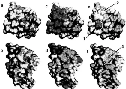
Figure 1. (a) Crystalline habit and growth, for example for this bismuth crystal, is determined by minimization of interfacial energy. (b) Under certain conditions, a mix of polymers can separate, or demix, driven by interfacial energy. Here a spun-cast film of polystyrene and poly(methyl methacrylate) form a striking pattern after demixing.5 _(c) Protein folding is another natural process driven by interfacial energy. In conceptual 2-dimensional lattice models6_{, hydrophilic residues (black beads) aggregate in the protein's} interior while hydrophilic groups (white beads) adorn the exterior. (d) An actual protein has a far more complex surface, however. Here, hydrophobin is shown from two angles.7 The shading represents hydrophobic groups (blue), hydrophilic groups (red) and intermediate groups (white). (Images taken from sources without permission, with the exception of (a), taken from wikimedia.org under the Creative Commons license.)

Interfacial energy also plays a vital role in another area of materials science-colloidal systems and dispersions, and largely determines their formation, resultant stability and

(12)

coalescence behavior.' 9 Here, interfacial energy is again treated as a function of the identities of the two abutting materials. However, since surfactants are commonly present at these interfaces and exhibit a large impact on interfacial energy, the role of the surfactant is included in the expression for interfacial energy as a function of concentration and the identity of the surfactant."," It is important to note that because in general the surfactants present at the interface largely lack structure and are randomly distributed, the interfacial energy can again be treated isotropically with satisfactory results. In more complex surfactant systems, especially those involving multiple components, interfacial energy is approached as a function of the components' identities and concentrations, and curvature of the interface. Interestingly, we note that the importance of a structural parameter can be seen in these systems: surfactants individually are viewed as having a structure, and not simply as point-like objects. Thus we see a nascent understanding that orientation of these objects is important and that each component (hydrophilic head and hydrophobic tail) is seen as distinct and, at least conceptually, having two different interfacial energies.

Another field in materials science where interfacial energy plays a prominent role is polymer science. Mixtures of polymers may undergo morphological changes driven by differences in interfacial energy in polymer demixing.5_"5 _{Here the polymer chains phase}

separate to reduce total interfacial energy. Much recent work has been focused on designing block copolymer systems that spontaneous self-assemble to generate a large variety of patterns and shapes as a foundation for more complex assemblies.16-19

(13)

Within the field of biology, the infamously difficult question of protein folding can be reduced to an attempt to minimize interfacial energy. In early conceptual models of the progression of protein folding20_-2 3_{, each residue, or amino acid, of a protein was labeled}

as either hydrophobic or hydrophilic, or equivalently, low- or high-interfacial energy. The interfacial energy of the entire protein was sequentially reduced by folding the protein to reduce the total number of residues exposed while maximizing the ratio of hydrophilic residues to hydrophobic residues on the exterior. While this model is simpler than the more complex computational models developed since, it is the common intuitive model for protein folding. Furthermore, the idea of grading each residues' relative hydrophobicity or hydrophilicity, or hydropathy, individually is still common today,24 25_,

and has been refined via the development of a numeric hydropathy scale that quantitatively relates the residues.23 26 A common method of presenting the morphology of a protein displays a mesh of the surface accessible surface area of the protein which is colored based on the relative hydrophilicity of the nearest residue.27

The conceptual insight to treat interfacial energy per residue was the key to beginning to understand the behavior of these complex systems. The growing complexity of a system under study is often accompanied by a decrease in the surface homogeneity. For such systems, especially those whose structure and function are strongly dependent on interfacial energy, the assumption of a constant interfacial energy for the entire system becomes questionable and the importance of structure in interfacial energy becomes apparent. Biological systems are inherently patchy at the molecular scale and many artificial systems are beginning to exploit such patchiness to direct self-assembly and

(14)

28

control material behavior. Just as an understanding of crystallographic growth would have been impossible for not the insight that the crystallographic orientation of a crystal's facet determines interfacial energy in addition to the composition of the crystal, a thorough understanding of the behavior and design of materials with structured interfaces is impossible without the development of a theory of interfacial energy that includes structural information.

1.3 Surface Energy vs. Interfacial Energy, the Work of Adhesion and other Definitions

Before further examining the theoretical development of interfacial energy, it would be helpful to define and demonstrate several terms and the thermodynamic relations between them. The materials used to develop these descriptions must be assumed to be isotropic and continuous, but may be taken to be liquids, gases, or solids, with the only exception that interfaces cannot exist between two gases.

The work of cohesion of a material, denoted W,1, is defined as the work required to

divide a material to produce two new surfaces of unit area in a vacuum (Fig. 2). As this produces two new units of area of surface, half of the work of cohesion is equal to the surface energy (yi) of the material. If two dissimilar materials are separated, the energy per unit of area is defined as the work of adhesion (W₁₂). Whereas the surface energy depended on the identity of one material, the work of adhesion is a function of the identity of two materials.

(15)

Work of Adhesion

1

1 Wu

7 W1

2 =

-

W

1

+

-VW

2 2

-

7Y12

2

1

711= -Wu 712 = 711

+

722 - W 1 2

2

Figure 2. The work of cohesion (left) is the energy required to separate a material from itself to generate 2 new units of surface area. The energy required is twice the surface energy. The work of adhesion (right) is the energy required to separate two distinct materials. The work of adhesion is the difference between the sum of the materials'

surface energies and their interfacial energy.

Interfacial energy is defined as the energy per unit area required to produce an interface between two materials. The expression for interfacial energy is:

Y12 = 71 + 72 - 1412 (1.2)

where y1 and 72 are the surface energies of each material, and W12 is the work of adhesion for the two materials. To understand the origin of this expression, it is important to consider the formation of an interface in vacuum. To form an interface, a unit area of each material must first be created; this energetic cost is simply the sum of the surface energies of each material. The attractive interaction between these new surfaces upon joining them to form the interface performs work (W12). Thus the energy required to form an interface is equivalent to the difference between the work required to form the

(16)

individual surfaces and the work returned to the system upon joining them. In this thesis, the interaction between a liquid and a solid will be expressed in terms of the work of adhesion rather than reporting the interfacial energy directly, due to the direct applicability of the Young-Dupr6 equation (Eq. 1.21) and its specificity in describing the attractive interactions. The interfacial energy may be viewed as an expression with two terms that describe the individual materials and a third term, the work of adhesion, that captures the interaction between these materials.8

As a final note: surface tension and interfacial tension are commonly conflated. The surface tension (or surface energy) of numerous materials is often presented in literature but it is important to remember that unless the measurements were performed under vacuum, the measured values more accurately describe the interfacial tension (or energy) of the interface between the material and the ambient atmosphere. Interfacial tension is thus a more apt term, but it is commonly reserved for the tension of an interface between two liquids.8

1.4 Thermodynamic Treatments of Interfacial Energy

J. W. Gibbs was the first to develop a thermodynamic model of the behavior of interfaces. While significant advances have been made in the knowledge of interfaces, Gibbs' concepts are still commonly referenced and are the foundation of all current theory.8,29-31' Gibbs' conceptual model of an interface was an infinitesimally thin layer between two phases that could be described by its area and curvature. On either side of this layer, or dividing surface, the materials are homogeneous and uniformly distributed

(17)

and at the dividing surface itself, an abrupt transition from one material to the other occurs. The interfacial tension would act in plane at this dividing surface.32

Such a model necessarily contains several assumptions, and it is important to note these assumptions and how they impact the nature of the interface. First, and most obviously, the interface itself has no structure-it is not a volume but a geometric boundary. Second, by assuming both substances are homogeneous, the interface is entirely isotropic and therefore does not contain structure. Finally, this treatment neglects the molecular nature of the materials and the nature of the interactions between molecules of the same and different phases.

In 1937, Fowler attempted to incorporate the concept of intermolecular forces into a theory of interfacial tension.3 3 _{His theoretical system was a planar interface of a vapor in}

contact with a liquid. An analytical expression was developed for the surface tension that required knowledge of the potential between two particles in the system and the distribution function of each material. This formulation was shown to yield a poor approximation of the surface tensions of argon and mercury. He conjectured that interfacial tension might depend on structure within the liquid. In the example given, this structure was conjectured to be highly ordered and crystalline in nature, with planes of varying bond density. Such structure does not exist in liquids and is relevant only to solids. This treatment attempts to incorporate intermolecular forces, but it still assumes an isotropic and homogeneous interface.

(18)

R. C. Tolman returned to a purely thermodynamic treatment and refined Gibbs approach by considering the structure of the interface.3_{' This conceptual model is especially}

notable because it serves as the basis for a majority of refinements made since to the structure of a liquid interface.34

Rather than confining the transition between phases to occur abruptly at a dividing surface, in Tolman's model, the transition occurs over a finite volume whose thickness was conjectured to be on the order of several molecular diameters. Within this transition region, the properties of each phase would deviate from the bulk properties as the dividing surface is approached. This treatment is more robust as it accounts for the finite extent of the interface, but cannot itself provide a means of describing the structure of the interface.

(19)

Laterally Homogeneous

Expanded View of Transition Region Transition Region - x N material 2 L2, P2 material 1 Pi

Gibbs Dividing Surface

2i

Density Profile Near Transition Region

Figure 3. (a) Tolman's model system is a sphere of material 1 embedded in material 2. (b) The dividing surface separates the two materials. The interface is assumed to not be diffuse. (c) The system exhibits spherical symmetry. Any variation occurs only along the outward direction. Variations within spherical shells are not accounted for with this treatment. (d) Along the radially axis, variations in the material density is allowed to occur. Hypothetical deviations from the bulk density of each material, indicated as the gray shaded regions, are shown as colored regions.

Tolman's theory is based on a two-phase system with spherical symmetry, as shown in Fig. 3a. A closer view of the interface is shown in Fig. 3b. The dark line is the dividing surface. As the transition occurs over a finite distance, there exist multiple ways to define the location of the dividing surface, and its location is selected to simplify the

(20)

mathematics. For this system, regardless of selection of the dividing surface, all surfaces will be spherical shells, and will lie parallel to each other. Here, the location of the dividing surface is taken as x=O on an axis emanating radially from the center of the system. The inner phase, composed of material 1, remains unperturbed by the interface until x=-b, where the equilibrium density and pressure are allowed to vary from the bulk. From x=-b to x=O, the density profile varies as shown in Fig. 3d. From x=O to x=a, a similar region exists where the properties of the outer phase deviate from that of the bulk at equilibrium. Fig. ld illustrates what the density profile through the transition region might look like. The gray shaded profiles represent the density profiles of each phase (material 1 on the negative x-axis, material 2 opposite) if the phases remained homogenous. The red and green shaded profiles represent the density deficiency or excess. From the geometry assumed in this treatment, namely spherical symmetry, variations in the liquids can only occur radially. As defining a surface with structure, or variation within a spherical shell, would defy the assumptions made in this treatment, this approach is unsuitable for describing interfaces at structured surfaces. It is however a convenient model to explain simple, homogeneous surfaces.

It is instructive to compare Tolman's treatment of the interface with the expression for the interfacial energy (Eq. 1.2). In Tolman's model, the system is comprised of a homogenous sphere of material 1 embedded in a homogeneous phase of material 2. The systems total energy can be expressed as the sum of the energy of each phase: Ei + E2.

When the transition layer is allowed to form, a correction term Es is added to the total energy. This derivation neatly parallels the derivation of and expression for interfacial

(21)

energy (Eq. 1.1) in terms of surface energies and the work of adhesion presented in the previous section. The work of adhesion does not only reflect the attractive forces between the surfaces, but also includes the work done when the interface restructures. The Es term in Tolman's theory, however, should not be interpreted as the energy of the transition region, but rather must be viewed as the energetic deviation upon relaxation from the system containing the non-relaxed, abrupt interface.

Tolman found that a necessary condition for equilibrium was

/I + # = Const. (1.3)

where i is the intrinsic chemical potential of component i and < is the potential due to external forces field. The forces experienced are the intermolecular forces present between molecules of the same phase, and between the two phases. Furthermore, if i is defined as

P

p (1.4)

where V is the Helmholtz free energy, p is the pressure, and p is the density, after substitution, taking the derivative with respect to position, and substitutingfx = d#/dx we find the expression:

d p dp 1dp d45

- -+-

+-=0

dx p2dx p dx dx (1.5)

The imbalance of forces near the interface is responsible for changes in density and pressure in the transition region. Away from the transition region, the potential due to intermolecular forces is constant and Eq. 1.4 reduces to pu=const. The physical origin of

(22)

the interfacial energy or tension can now be succinctly stated: unbalanced forces acting on the fluid at the interface change the local density from that of the bulk material, and this altered density in turn changes the average cohesive force at the interface, the sum of which is the interfacial tension.

The thickness of the transition region, even at the time Tolman formulated his theory, was known to be only a few molecular diameters. The applicability of thermodynamic concepts is questionable over such minimal extents, especially when large variations occur. The thermodynamic treatment rendered by Tolman did not provide an understanding of the actual structure of the liquid interface, and such a conceptual understanding would require the development of a theory that could incorporate molecular theory.

A statistical mechanical basis for surface tension was developed in 1949 by Kirkwood and Buff30 that incorporated the variations in density local to the interface. Similar to Fowler, they utilized a planar interface separating two fluid phases. While they did permit variations from the bulk density, they assumed the density only varied as a function of distance from the dividing plane. Interfacial tension was calculated as the stress acting at the interface necessary to offset the pressure variations that would occur in each phase if the interfacial tension were not present. The expression for interfacial tension is similar to an expression developed by Tolman,

(23)

The authors are careful to point on that an assumption made by Tolman, that the pressure p'(z) can be equated to the pressure of the bulk material at the same density, is inaccurate and must be treated using statistical mechanics. While the Kirkwood-Buff theory is capable of reproducing the same results as Fowler by reducing the transition region to a plane, it is more general since it makes no stipulations of the region local to the dividing surface. The theory is shown to reproduce the findings of Tolman, as well as approximate the surface tension of liquid argon.3 0

More recent numerical treatments have built on the knowledge of the interfacial structure. Notably, several attempts to clarify the density profile of gas/liquid and liquid/liquid interfaces using Monte Carlo or molecular dynamics simulations have been made. The success of these attempts is strongly dependent on the accuracy of the force field used. Additionally, the impetus behind many studies in this area is greater knowledge of the nature of liquid/vapor phase transitions, and not the measurement of mechanical properties such as interfacial tension.34

1.5 The Origin of Interfacial Energy: Intermolecular Forces

Even the earliest treatments of interfacial energy identified the lack of symmetry and the resulting force imbalance at the interface as the cause of interfacial tension. In the prior century, significant work has been directed at cataloguing and explaining the varieties of forces that can exist between molecules. All of the intermolecular forces are electromagnetic in origin and stem from interactions between dipoles or charges. A liquid whose molecules contain permanent dipoles is said to be a polar liquid, whereas a liquid that does not is termed non-polar. Non-polar liquids and polar liquids alike can

(24)

experience van der Waals forces due to fluctuations in the distribution of charge resulting in temporary dipoles, while interactions between two permanent dipoles (Keesom forces) and permanent and induced dipoles (Debye forces) require either both or one of the molecules to be polar.8

As the interfacial tension is so strongly determined by the nature and strength of the forces acting at the interface, efforts were made to decompose the interfacial tension according to the forces responsible. One early and rather successful attempt was made by Fowkes, who regarded interfacial tension as the sum of several components, each attributable to a class of forces. For instance, the interactions present in liquid mercury could be classed as either metallic bonds or dispersion forces. In water, the interactions were either dispersion forces or polar interactions, which included hydrogen-bonding effects. As hydrocarbons are a non-polar liquid, their interfacial energy is wholly attributable to dispersion forces and only contains this one term.

Hg Hq + 7Y Hq _(1.7)

?H20 H2O + 71H20 (1.8)

d

(25)

Figure 4. Fowkes' model of a liquid-liquid interface assumes an interface comprised of two monolayers of each liquid (demarcated by horizontal lines). Each monolayer experiences two forces: one toward their respective bulk, equivalent to the surface energy and a second toward the interface due to dispersive forces, with the magnitude as calculated by the Berthelot relation.

Fowkes employs a simplistic model of the interface as two abutting monolayers of liquid backed by their respective bulk phases. The interfacial tension is taken to be the sum of the attractive forces parallel to the dividing surface experienced within each monolayer of liquid (see Fig. 4). If one of the materials is taken to be non-polar, the only interaction that can occur between the two materials are van der Waals forces. The magnitude of this interaction is taken to be the geometric mean of each phase's dispersion component by the Berthelot relation. (In a similar route, Girifalco and Good36 _{had previously attempted} to calculate the work of adhesion directly from two materials' interfacial energy. This approach was unsuccessful as it ignored the nature of the interactions present.) In this model, each monolayer would experience its full surface tension drawing it toward the bulk and the dispersion interaction previously calculated drawing it toward the dividing

(26)

plane. Summing the contributions for both monolayers yields the total energy of the interface:

6d d

712 = 71 + 72 - 2 1 72 _(1.10)

Here the superscript denotes the fraction of surface energy from dispersive interactions. While this derivation oversimplifies the structure of the interface and liberally employs the surface energy as an additive force, the resulting expression is useful to examine as it parallels the expression given for the interfacial energy, with the work of adhesion given by the attractive force explained previously, 2 _{. Experimentally, this formulation was} tested by measuring the spreading of various hydrocarbons on water and mercury. Spreading occurs when wetting a surface is so favorable the contact angle is nonexistent, causing a drop to spread completely wetting the surface. With a hydrocarbon (HC) on water, this will only occur if the surface tension of water is greater than the sum of the surface tension of the hydrocarbon and the interfacial tension of their interface (see Fig. 5), or more succinctly if:

7YH2O - (7HC + YH2O/HC) > 0 (1.11)

The expression on the left hand side is termed the spreading coefficient and its sign indicates whether or not spreading would occur. By applying the previous equation (Eq. 1.10) to simplify the spreading coefficient, an efficient method of quantifying the dispersion component of water emerges. Note that this simplification is possible because it is assumed the surface tension of hydrocarbons is purely due to dispersive interactions. If the simplified coefficient is positive,

(27)

2 7HC 2o -YHC>0 (1.12)

spreading will occur. Indeed, the hydrocarbons with surface tensions less than H2o, 21.8 dynes/cm, are found to spread.37 _{Curiously, it was also found that this relation only held} true for purely aliphatic hydrocarbons. Aromatic hydrocarbons were found to interact with water more strongly than would be expected from purely van der Waals interactions. As aromatics are more polarizable than aliphatics, dipole-induced dipole related forces would be expected for these solvents.8

~ '7HC

YH2 0T 2OYH0/HC

Figure 5. The sign of the spreading coefficient determines if a liquid will spread on a liquid surface. It is derived by consideration of the forces acting on the three-phase line. For a very wetting liquid with a negligible contact angle, the interfacial tensions act in the same plane leading to Eq. 1.11.

The concept of spreading was also central to an attempt to understand the wettability of solid surfaces by Zisman.38 _{Spreading on a solid surface occurs when the contact angle of} a drop is zero, or equivalently when its cosine is one. If spreading occurs, a liquid drop would spontaneously spread to cover the surface; this state is termed complete wetting. By plotting the cosines of the contact angle for various hydrocarbon liquids on a given surface against their surface tensions, the surface tension when complete wetting begins could be extrapolated. As the liquids used were mostly aliphatic hydrocarbons (namely n-alkanes), the discrepancy that would occur when using polar solvents was not readily

(28)

apparent. Due to the number of interactions between a liquid and solid (H-bonds, polar forces, dispersion forces), the wetting behavior of a solid cannot be reduced to a single parameter, such as the critical wetting surface tension.

Owens and Wendt continued the analysis of Fowkes, and extended it to interfaces between phases which can interact via hydrogen bonding in addition to dispersion forces.3 9 _{In this case, the surface tension of water could be written as:}

7H20 7H0 -H20 _(1.13)

Using twice the geometric mean of each component as before, the work of adhesion can be expressed as:

i~ ~-I y 2 <_

r4'p

(1.14)

where the final term represents the work of adhesion. Here, the subscript represents the phase (s=solid, 1=liquid). If no superscript is present, the term represents the total surface energy. Otherwise, the superscript represents the surface energy component due to dispersive (d) or hydrogen-bonding (h), interactions. By using two different solvents that are fully characterized, i.e. the dispersion and hydrogen-bonding components of each liquid are known, measurements of the liquids' contact angles on a solid surface can be used to calculate the dispersion and hydrogen-bonding components of the surface. In the original publication, this method is shown to provide reasonable values.

Later work sought to refine the calculation of the interactions at the interface. The classification of a material's ability to hydrogen bond by a single coefficient is rather

(29)

inaccurate. It is well understood that hydrogen bonding occurs between a hydrogen bond donor and a hydrogen bond acceptor, and that a substance's ability to perform one role is not equivalent to the ability to perform the other. Therefore, a further distinction must be made in the decomposition of the surface energy terms to describe attractive interactions of a substance due to its role as a hydrogen bond donor or acceptor.4 _'4₁_{This further}

specification appears as another term in the interfacial energy:

2( j>1 2 'i14- ₂ Y~~

(1.15)

Here the subscript denotes the phase, and the superscript indicates the donor (+) and acceptor (-) components of the acid-base (AB) interaction. The necessity of clearly delineating the varieties of forces acting at an interface demonstrates that numerous factors must be taken into account and that the behavior of interfaces cannot be easily

summarized by a single factor.36,38,42

Recent work has challenged the need to examine the forces operating at the interface and has supported the view that interfacial energy can be reduced to a single parameter. Kwok et al. has argued against the validity of decomposing the interfacial energy by nature of intermolecular forces and has instead claimed that the contact angle is solely indicative of the surface tension of the probe liquid. In a series of studies, the advancing contact angle of drops of numerous liquids on a silicon wafer coated with a fluorinated compound was measured. Of the 30 liquids studied, 9 displayed constant contact angles as the drop size increased while the remainder displayed stick-slip motion.43 In another study by the same researchers, the interfacial tensions of immiscible liquids were studied to test the validity of Van Oss's approach. If a positive interfacial energy is calculated, it

(30)

was posited that the liquids should be immiscible, and vice versa. It was found that several liquid pairs with positive interfacial energies were in fact miscible.4 4

The spreading behavior of the first study is consistent with pinning of the three-phase line at defects on the surface. (See section 1.9.) From the published data, a large range of angles was observed43_{, yet, for a given liquid, the minimum angle achieved when the} drop becomes unpinned and advances, is essentially constant. This indicates the contact line pinning with the drop periodically relaxing to a non-pinned shape. Such measurements were excluded from Kwok's treatment, and only those that spread evenly were included. Furthermore, the use of a fluorinated substrate was a poor choice as fluorinated materials have unique interactions with both 'polar' and 'non-polar' materials. The second study44 _{on miscibility is more experimentally sound but has}

theoretical pitfalls. While Van Oss suggests that the interfacial energy of two liquids can be estimated knowing the nature of the intermolecular interactions present, it is never suggested that such calculation is an exact form or that it can completely capture the behavior of the liquids at the interface. Finally, the assumption that two liquids will be miscible if the calculated interfacial energy is zero or negative is flawed as the entropic contribution to the free energy of mixing is completely ignored. For these reasons, this thesis will adopt the conventional view that the strength and nature of interactions at the interface are critical to understanding wetting behavior, and furthermore, wetting behavior cannot be summarized by a single parameter.

(31)

1.6 Relating Experiment to Theory

Several methods exist for determining the interfacial energy of a solid liquid interface. The most common is goniometry, where the angle of contact of a small drop is measured and from which the interfacial tension can be calculated. In addition, there exist force-based techniques that can directly measure interfacial tension by recording the force exerted upon a probe in contact with a liquid. This section concludes with a novel technique developed in the scope of this thesis that measures interfacial energy with a scanning probe microscope.

The original development of a measurement of interfacial energies was made by Young in 1805.4 This method, commonly referred to as goniometry or more commonly contact angle measurements, is commonly used today. The basic technique can be described as thus: A drop of limited volume is placed upon a flat surface to be analyzed. Upon contact, the drop will attain an equilibrium angle with the surface. This angle is called the contact angle and describes the relative interfacial energies of the solid/liquid, solid/vapor, and liquid/vapor interfaces.

(32)

Figure 6. (left) Young related the magnitude of the interfacial tensions at the three-phase boundary of a sessile drop on a flat surface to the contact angle between the liquid-air and solid interfaces. (right) This equation must be employed judiciously as the liquid-solid interfacial tension calculated is only representative of the annular region immediately neighboring the drop's boundary. The differential area considered in the derivation is shaded.

In Young's original derivation, the equilibrium angle was calculated via force balance requirements at the 3-phase line. This derivation is briefly summarized in Fig. 6, and it yields the familiar equation:

7Se = 7/9 + 7Icos(9) (1.16)

While the end result is the same, it is instructive to consider an alternate derivation of Young's equation8_,4 6 _{that is posed in terms of an energy balance. While volume is being}

added to the drop, the 3-phase line will advance requiring the advancement of two interfaces (solid/liquid and liquid/vapor) and the retraction of the solid/vapor interfaces. The relationship uniting the interfacial energies and their differential areas shown in Fig. 6 is given below:

(33)

The contact angle is measured at equilibrium, so the drop volume is taken to be constant. The differential areas can be simplified by realizing that the change in As, is opposite to the change in As,. Additionally, the differential area dAi, can be geometrically related to dAsi via the geometric relation:

dAi, = dAsicos(0) _(1.18)

Upon substitution into the original equation, and requiring all derivatives of energy to be zero at equilibrium, we find the original Young's formula (Eq 1.16). While the end result is the same, the derivation reveals an important caveat of Young's formula. The contact angle measured does not reflect the interfacial energy of the entire wetted solid/liquid interface. Instead, it is only sensitive to the interfacial energy of an annular section local to the 3-phase line depicted in Fig. 6.

As described in Section 1.3, another important quantity that will be used to relay the measurements made in this thesis is the work of adhesion, Wsi. The expression for the work of adhesion is derived from the definition of interfacial energy (Eq. 1.19) with Young's equation (1.20), and is termed the Young-Dupre relation8 (Eq. 1.21). In contrast to the version of Young's equation given above (Eq. 1.16), Ys replaces ysv and yi replaces yIv in the version below (Eq. 1.20) due to the negligible influence of the gaseous phase on the interfacial energies of the liquid and solid.

7 78 + 71 Ys - WS1 (1.19)

7S = YS + -yicos(6) (1.20)

(34)

In this thesis the work of adhesion will be the preferred means of expressing interfacial measurements. As shown previously, the work of adhesion is directly related to the interfacial energy and describes the strength of the interaction between the solid and liquid. Furthermore, it is experimentally attractive, as its calculation requires only measurement of the contact angle and the probe liquid's surface tension. An understanding of this expression will also simplify interpretation of the following discussions on the wetting of non-ideal surfaces.

1.7 Extending Young's Equation

The surfaces in the derivations previously described are assumed to be perfectly planar and perfectly homogenous. However, only very few surfaces of scientific and technological interest will have a roughness in which the flat approximation would suffice. To allow measurements on textured surfaces, it is necessary to adjust the previously derived formula to incorporate the effect of surface roughness.

The first and most commonly used correction for roughness was developed by Wenzel in 1936.4 The roughness is characterized using a term r, the roughness factor, defined as the ratio of the area of the actual surface to the geometric or projected surface. Young's equation can be recalculated using this factor to yield:

r(,ysv - N) = 'y1cos(O) _(1.22) The measured angle corresponds the macroscopic angle measured. It is straightforward to relate the macroscopic contact angle measured on a rough surface to the contact angle

(35)

that would be measured on ideally smooth surface of the same material. The observed contact angle is related to the ideal contact angle via the relation:

r * COS(Oideal) = COS(Oobserved) _(1.23)

From this it is clear to see the effect roughness has on the contact angle: for surfaces that have a contact angle less than 900, increasing roughness reduces the contact angle, or increases wetting. For surfaces with contact angles greater than 90', increasing roughness increases the contact angle.

It is important to understand the origin of the r factor. Roughness is often reported as the root mean square (RMS) of the deviation from a surface's average height, as measured using profilometry. Wenzel recognized this measure did not satisfactorily capture the effect on wetting and highlighted a study in which samples exhibited the same contact angle yet differed nearly two orders of magnitude in RMS roughness.48 _{The effect of} roughness is better captured from calculating the total area of the interface. Such a measurement was impossible when Wenzel's work was originally performed but is now achievable with scanning probe techniques.

Furthermore, Wenzel makes a salient point that the "type" of roughness is absolutely critical.48 _{For demonstration, he considers a grooved surface that resembles a sawtooth} curve. Every surface with this profile has the same r-factor: 1.41. However, the importance of the scale of the effects can be seen with a simple thought experiment. A surface that is otherwise smooth with the sawtooth profile of a period greater than the drop size would report a contact angle equivalent to the angle that would be measured on

(36)

an ideally flat surface. Furthermore, decreasing the period of the roughness below the size of the liquid molecules would produce a surface whose solvent accessible area is equivalent to a flat surface. Thus, at both extremes of the length scale, the roughness of the surface cannot be probed by the liquid.

Furthermore, the type of roughness has a significant effect on the local contact angle. Early attempts to understand contact angle hysteresis sought to link geometric variations experienced by the three-phase line while advancing and receding to the macroscopic angle measured. As hysteresis is observed with surfaces that can be practically considered perfectly flat, this model is only one plausible cause of hysteresis. Roughness can also influence the anisotropy of a surface's wetting behavior. Grooved49_'50 _or

striped5

1 surfaces show that droplets do not present the same contact angle in both

directions. Surfaces can be fabricated with strongly anisotopic surface patterning to control the motion and growth of a liquid in contact with the surface. The roughness experienced by an expanding drop is proportional to the projected length of the local surface perpendicular to the contact line.

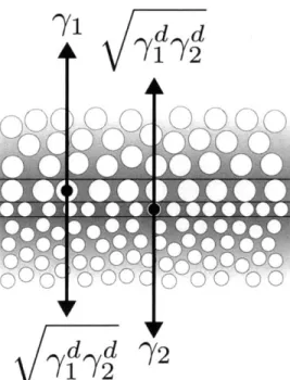
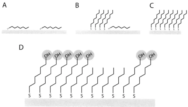
Wenzel's work was primarily motivated by a study of waterproofing materials, generally applied to flat surfaces. Cassie and Baxter, also studying waterproofing materials, sought to extend Wenzel's theory to porous surfaces, namely fabrics that had been treated with a water repellant coating.53 Porous surfaces in contact with a drop of water do not present a simple interface between a solid and a liquid. Rather, the liquid forms a mixed interface: a solid/liquid interface is formed where the drop contacts the surface, but a liquid/vapor

(37)

interface exists in the pores or voids in between fibers. If

fi

is defined as the surface fraction of the solid/liquid interface and

f

2 is defined as the surface fraction of the

liquid/vapor interface, with

f+f2

= 1, the solid interface's contribution to Young's equation can be treated as the weighted average of its components. Writing the energy to advance the solid/liquid interface a unit area in terms off, andf2, we find:

Eadv = (Ysv - 'Ysv) + f2Ylv (1.24)

The first term, is a product of the solid/liquid interface fraction

fi

and the interfacial energy difference of the interface being formed between the liquid and solid, and the interface being destroyed between the solid and vapor. The second product reflects the energy required to extend the liquid over the pores, creating a liquid/vapor interface.

For a flat surface, Young's equation can be rearranged to give an expression for Eadv:

7ysV -7s1 = 7vCOS(Oobserved) = Eadv (1.25)

By equating the two equations, an expression for the macroscopically measurable contact angle can be found:

'YlCOS(Oobserved) = fi(s1 -- Ysv) ± f2'Ylv (1.26)

Just as with Wenzel's formula, it was possible to translate the observed angle to the angle that would be measured on a perfectly smooth surface, it is possible to relate the material's contact angle to the measured angle:

7sv -- 73s

COS(Oideal)

-(1=27)

7brv (1.27)

(38)

Iff2, the fraction of the interface composed of the interface spanning pores, were zero, the previous equation reduces to Wenzel's formula, with

fi

replacing r. The Cassie-Baxter relation is used to understand the wetting observed on superhydrophobic surfaces.5456 These surfaces, which both exist naturally and are engineered, demonstrate contact angles with water exceeding 1500. The characteristics in common with all of these surfaces are a high degree of roughness and a surface that is intrinsically non-wetting. The non-wetting surface prevents the liquid from being drawn into the surface via capillary action, and the extreme roughness only permits a fraction of the droplet to contact the solid. As the fraction of the interface that is liquid/vapor increases, the observed angle approaches 1800, independent of the material's intrinsic wettability. Because of this property, the production and design of such surfaces is a technological goal.

While the Cassie-Baxter expression was developed to described rough surfaces that could trap air, it can be used more generally as an expression of interfacial energy for a heterogeneous surface. This treatment has been successfully applied to systems that possess heterogeneous surfaces containing domains of different chemical composition and wetting behavior.51'57-60 There have been extensions made to this model to further increase its accuracy by accommodating for the geometry of the surface51_'57_{; however,} these extensions are not generalizable and are system dependent. For this reason, the standard Cassie-Baxter equation will be treated as the benchmark model for expressing interfacial energy.

(39)

1.8 Experimental Determination of Interfacial Energy

Contact angle remains the most common and most accessible method of measuring the interfacial energy of a solid/liquid interface. This technique has been described in the preceding section and remains straightforward to perform. It must be noted that the measurements obtained are only valid if certain conditions are met. Only drops that are clearly advancing or receding and are not affected by surface imperfections (Section 1.9.) are admissible.

Tensiometry is a mechanical technique for measuring interfacial tension. This technique directly measures the force exerted on an interface; by lowering and raising a specimen in and out of a liquid, interfacial area is created and destroyed, respectively. By canceling the buoyant force exerted by the liquid on the object, the force due to interfacial tension can be accurately measured.61 The specimen must be smooth and possess a constant perimeter along the immersion direction as the interfacial tension is directly calculated by dividing the force measured by the sample's perimeter. Tensiometry can also be used to directly measure the surface energy of a liquid: using a perfectly wetting calibration standard, the resulting interfacial tension will exactly represent the surface tension of the liquid being measured. Two standard probes exist for conducting this measurement: the Wilhelmy plate and the DeNuoy ring, which are functionally equivalent but with different geometries.

Tensiometry is an attractive method of measuring interfacial tension because it easily allows measurement of advancing and receding angles. While the primary limitation in measuring contact angle hysteresis in sessile drop technique is ensuring the drop

(40)

perimeter is evenly advancing and receding, this is automatically accounted for by the geometry of the interface under study in tensiometry. Furthermore, tensiometry is capable of measuring highly wetting surfaces that exhibit low contact angles that are difficult to measure using goniometry.

The final technique to measure interfacial energy was recently developed by a collaborator and myself. This technique utilizes scanning probe microscopy to generate a mapping of interfacial energy over a nanoscale region, and it relies on measuring the energy dissipated while imaging a liquid/solid interface. Details of this method will be given in the following chapter. This technique is especially useful as it establishes the interfacial energy away from the three-phase contact line and ensures the region measured is free of defects.

1.9 Measurement Difficulties: Hysteresis and Pinning

The measurement techniques discussed so far have presented the measurement of contact angle as a straightforward method that produces certain results. However, much care must be spent in the acquisition and interpretation of the data gathered as large errors can occur due to the unique challenges of measuring contact angle. While contact angle so far has been presented as a geometric feature resulting from the underlying physical interactions at the interface, its value for a given liquid-solid interface is not unique. Most surfaces can actually report a large range of values depending on the last motion of the three phase line, and this dependence on the history and current motion of the contact line is referred to as contact angle hysteresis (CAH). The advancing and receding angles represent the extreme points of this range of values. To ensure reliable measurements,

(41)

one requirement is that the direction of motion be confirmed. That is, to report contact angle values of a drop that is clearly advancing as advancing (and likewise for receding) and not simply the angle observed of a sessile drop on the surface.

One cause of CAH is the presence of defects on the surface being measured. Even surfaces that are close to perfectly flat can contain small imperfections, either hills or holes in the surface. These imperfections can pin the three-phase line preventing from evenly advancing (or receding) over the surface. Because such defects prevent a barrier to a spreading drop, they will cause the apparent contact angle to be greater than what it would be for an ideally flat surface. For a receding drop, the three phase line may be pinned at the defect and cause the contact angle to appear lower than what it ideally would be if the surface were smooth.

Pinning defects have been studied in great detail because they represent a problem in performing and interpreting measurements as well as a challenge in the design of microfluidic systems.62 The geometry, relative stability, and movement of drops on superhydrophobic surfaces is dominated by pinning at the numerous projections from the surface.63 Pinning defects however also present a means of engineering surfaces that present anisotropic wetting properties. By fabricating surfaces with oriented grooves or raised plateaus, the contact angle becomes dependent on direction, and such surfaces are of interest for directing the motion of liquids on surfaces.64

With regards to characterizing surfaces of unknown surface energy, it is ideal to reduce the probability of pinning. This is done by producing surfaces with few intrinsic defects and by exercising caution to not damage the surface prior to and during measurements.

The effect of nanoscale structure on interfacial energy

The Effect of Nanoscale Structure on Interfacial Energy

ARCHNES

FEB 0 8 2011

LIBRARIES

.

-

//

The Effect of Nanoscale Structure on Interfacial Energy

Jeffrey James Kuna

Contents Overview

Chapter 1: Introduction to Interfacial Energy ...

9

Chapter 2: Interfacial Energy of Patchy Surfaces ...

48

Chapter 3: The Experimental Systems and Methods ...

60

Chapter 4: Experimental Results...86

Chapter

5:

The Breakdown of Cassie-Baxter Theory and Considerations for

a N ew T heory ...

105

Chapter 6: Conclusions and Future Work ...

124

Appendix: Experimental Methods...134

Table of Contents

Figures and Illustrations

Tables

1

1

Wu

7

W1

-

W

+

-VW

-

7Y12

2

2

1

+

2

2i

+-=0

r4'p

(1.15)

fi

f

f+f2

fi

fi

_{The Breakdown of Cassie-Baxter Theory and Considerations for}