Measuring Longevity Risk for a Canadian Pension Fund

Texte intégral

(1)2011s-43. Measuring Longevity Risk for a Canadian Pension Fund M. Martin Boyer, Joanna Mejza, Lars Stentoft. Série Scientifique Scientific Series. Montréal Avril 2011. © 2011 M. Martin Boyer, Joanna Mejza and Lars Stentoft. Tous droits réservés. All rights reserved. Reproduction partielle permise avec citation du document source, incluant la notice ©. Short sections may be quoted without explicit permission, if full credit, including © notice, is given to the source..

(2) CIRANO Le CIRANO est un organisme sans but lucratif constitué en vertu de la Loi des compagnies du Québec. Le financement de son infrastructure et de ses activités de recherche provient des cotisations de ses organisations-membres, d’une subvention d’infrastructure du Ministère du Développement économique et régional et de la Recherche, de même que des subventions et mandats obtenus par ses équipes de recherche. CIRANO is a private non-profit organization incorporated under the Québec Companies Act. Its infrastructure and research activities are funded through fees paid by member organizations, an infrastructure grant from the Ministère du Développement économique et régional et de la Recherche, and grants and research mandates obtained by its research teams. Les partenaires du CIRANO Partenaire majeur Ministère du Développement économique, de l’Innovation et de l’Exportation Partenaires corporatifs Banque de développement du Canada Banque du Canada Banque Laurentienne du Canada Banque Nationale du Canada Banque Royale du Canada Banque Scotia Bell Canada BMO Groupe financier Caisse de dépôt et placement du Québec Fédération des caisses Desjardins du Québec Financière Sun Life, Québec Gaz Métro Hydro-Québec Industrie Canada Investissements PSP Ministère des Finances du Québec Power Corporation du Canada Raymond Chabot Grant Thornton Rio Tinto State Street Global Advisors Transat A.T. Ville de Montréal Partenaires universitaires École Polytechnique de Montréal HEC Montréal McGill University Université Concordia Université de Montréal Université de Sherbrooke Université du Québec Université du Québec à Montréal Université Laval Le CIRANO collabore avec de nombreux centres et chaires de recherche universitaires dont on peut consulter la liste sur son site web. Les cahiers de la série scientifique (CS) visent à rendre accessibles des résultats de recherche effectuée au CIRANO afin de susciter échanges et commentaires. Ces cahiers sont écrits dans le style des publications scientifiques. Les idées et les opinions émises sont sous l’unique responsabilité des auteurs et ne représentent pas nécessairement les positions du CIRANO ou de ses partenaires. This paper presents research carried out at CIRANO and aims at encouraging discussion and comment. The observations and viewpoints expressed are the sole responsibility of the authors. They do not necessarily represent positions of CIRANO or its partners.. ISSN 1198-8177. Partenaire financier.

(3) Measuring Longevity Risk for a Canadian Pension Fund* M. Martin Boyer †, Joanna Mejza, Lars Stentoft‡. Abstract In this paper we consider two particular Canadian defined benefit pension plans to illustrate the importance of adequate mortality forecasting on actuarial liabilities. An employer who sets up an employee defined benefit pension plan promises to periodically pay a certain sum to the participant until death. Both the employee and the employer finance these periodical payments during the beneficiary’s career. Any shortcoming of funds in the future is, however, the employer’s responsibility. It is therefore essential for the employer to be able to predict with a high degree of confidence the total amount that will be required to cover its obligations to the future retiree. If increases in life expectancy were predictable and taken into consideration when establishing retirement funds, assessing future liabilities would be riskless in that respect. Unfortunately, future survival rates are uncertain. On that account, pensioners may outlive their life expectancies and expose pension funds to longevity risk. We present different tools to hedge this risk and the potential cost for two Canadian public pension plans. Keywords : Cairns-Blake-Dowd model, Lee-Carter model, Pension Funds. JEL Codes: G22, G23. *. This research is financially supported by CIRANO. HEC Montréal and CIRANO, 3000, chemin de la Côte-Sainte-Catherine, Montréal QC, H3T 2A7 Canada. martin.boyer@hec.ca. ‡ HEC Montréal and CIRANO, 3000, chemin de la Côte-Sainte-Catherine, Montréal QC, H3T 2A7 Canada. lars.stentoft@hec.ca. †.

(4) 1. Introduction. Although we would all like for our lives to last longer, we would need to do so without running out of funds once we’re old and grey. Lacking financial resources is, however, one of the pernicious effects stemming from longevity risk, which we define as the risk that a population lives longer than anticipated. Put differently, longevity risk is the risk that the annuitants’ anticipated life expectancy is less than their actual life expectancy so that not enough money has been put aside to fulfill the annuitant’s future consumption needs. Obviously, longevity risk greatly affects the profitability of institutions that offer lifetime pensions. But longevity risk also consistently affects all levels of society, from individuals to companies and governments: • To compensate for longevity risk alone, it has been estimated that companies should increase their pension fund provisions by approximately 4%. • For the Government of Québec, the implicit unfunded liability of the Régie des rentes du Québec is 172 billion dollars. The unfunded deficit for the government employees’ various pension funds is 53 billion dollars. • At worse, individuals risk running out of money after retirement; at best, they do not know how much they should save today to adequately finance their retirement. Two elements highlight the importance of longevity risk: the amount of money at stake (unfunded liabilities for insurers and retirement funds represent more than 1,800 billion dollars in Canada alone) and the systematic underestimation of the mortality rate. Turner (2006) reports that life expectancy has systematically been underestimated by about 18 months for each decade. Clearly, the decrease in the mortality rate has important consequences on the viability of public and private pension funds, as well as on life insurance companies, since underestimating life expectancy will lead to insufficient accumulations. The importance of longevity risk and exposure to it has recently been recognized by the international accounting standards board, which has begun to tackle the problem of how to disclosure longevity risk in financial statements (see Fujisawa and Li, 2010). One of the particularities of aggregate longevity risk is its non-diversifiable nature (see Milevsky et al., 2006). As long as the aggregate mortality rate is known, individual deaths remain independent random variables. The Law of Large Numbers can thus be applied: the larger the sample population, the more the latter’s life expectancy tends toward that of the total population, and the more certain the sample’s mortality rate. If the aggregate mortality rate is uncertain, then the Law of Large Numbers no longer 3.

(5) applies as individual deaths are no longer independent variables. Indeed, for the aggregate mortality rate to evolve, individual deaths must, on average, evolve in the same direction. They must therefore be partially correlated. As a consequence, aggregate longevity risk is a non-diversifiable risk. Aggregate longevity risk can thus be considered as a good and a bad thing for society. It is a positive risk insofar as the population, on average, lives longer because of improved sanitary conditions and medical innovations. Demographically speaking, this is positive progress. Financially however, the risk is negative. Indeed, the retirement systems of developed countries rely on aggregate mortality rate forecasts. These are generally in the form of the payment of a pension until the individual deceases. Thus, when the life expectancy of a cohort of pensioners exceeds forecasts, the retirement system must pay in excess of the level initially projected. It is then exposed to the risk of lacking the capital needed to meet its financial commitments. Also, given the non-diversifiable nature of aggregate longevity risk, it is difficult for retirement systems to hedge themselves against this risk. Considering the size of the risk exposure and its undiversifiable nature, it has been argued that the only way to potentially manage this risk is by drawing on the capital markets. Potential losses arising from longevity risk are so large that they would likely be devastating for the insurance industry; for capital markets, however, such losses are not uncommon. Thus, capital markets have the ability to absorb large amounts of risk, much more so than the reinsurance market. This ability stems from the fact these markets are very large and that their existing portfolios have, in general, virtually no exposure to this type of risk. For the participants in the capital markets a potential benefit is that assuming this type of risk could offer a new class of assets to money managers. Once again the reason is that such assets have zero or negligible correlation to their portfolio of financial assets. Thus, having exposure of this kind of risk can increase the level of diversification in their overall portfolio and therefore decrease the volatility of their entire book of business. For this reason the capital markets have started to develop products and solutions that allow financial institutions to invest in mortality and longevity. The primary example of such a product is the mortality swap whereby one party will pay a measure of expected mortality and in return will receive a measure of actual mortality experience. More recently investment banks have started to look more closely at other ways to sell longevity exposure in the capital markets. As a result, mortality indices are being developed by the likes of Credit Suisse, JPMorgan and Goldman Sachs. The JPMorgan index for instance, called LifeMetrics, provides data for evaluating current and historical levels of mortality and longevity. The immediate advantage of such indices is that they enable pension plans, insurers and reinsurers to measure mortality and longevity risk in a 4.

(6) standardized manner. For such contracts to be a success both hedgers and speculators will have to find it attractive to transact in the market, and both will need to become familiar and comfortable with the use of derivative products. In this paper we consider Canadian defined benefit pension plans and stress the impact of adequate mortality forecasting on actuarial liabilities. An employer who sets up an employee defined benefit pension plan promises to periodically pay a certain sum to the participant until his or her death. Although both the employees and the employer finance may be asked to fund the plan during the beneficiary’s career, any shortcoming of funds in the future is ultimately the employer’s responsibility. It is thus essential for the employer to be able to predict with a high degree of confidence the total amount that will be required to cover its obligations to the future retiree. To do so, several assumptions must be made, specifically, the rate of return on the assets before they are liquidated, the amount of the periodic payment (based on the employee’s salary and indexation) and of course, the number of years the employee is expected to live after retirement (i.e., the number of years that benefits will be paid). All these factors have a very large impact on the actual cost of the pension plan and on its solvency ratio. The conditional life expectancy is particularly difficult to predict due to medical improvements. For example, in 1950, a 65 year-old Canadian male pensioner was expected to live another 14.1 years. In 2006, a male with the same characteristics would go on to live another 19.5 years. This entails a 5.4 years of additional payments. Of course, such mortality trends can be modeled to offer predictions on future life expectancy. The Lee-Carter model is a simple one-factor model that offers a good fit for mortality modeling over a wide range of ages. The model measures mortality rates on the assumption that they are perfectly correlated at all ages. A more appropriate model would incorporate a second factor to seize cohort effects, however. That is, not only a parameter that captures the trend in longevity improvement but also another that distinguishes the different age dynamics. Our paper will use such an approach base on the Cairns, Blake and Dowd model (the CBD model hereinafter). Boucher and Boyer (2009, 2010) implemented the CBD model to the Canadian mortality tables. They estimated the future increase in life expectancy of Canadian men and women aged 55 and over using data from the Human Mortality Database and measured the longevity risk associated with issuing immediate and differed annuities by a pension fund. They then applied the CBD model to the Royal Canadian Mounted Police’s pension plan. The choice of the institution was due to the fact that its actuarial report is publicly available and because contributors and retirees are homogeneous. The present value of the expected future benefits was calculated using the projected mortality rates as forecasted by the Office of the Chief Actuary (OCA). The present value was then compared to the one obtained using the results of the CBD model. 5.

(7) Given the results, the plan’s value-at-risk (VaR) was calculated for different levels of confidence in order to emphasize the uncertainty in future predictions. The objective of this paper is to update and verify the results obtained by Boucher and Boyer (2010). The CBD model is re-calibrated using the most up to date data from the Human Mortality Database. The results of the regression are then applied to the RCMP’s pension plan and also to the Canadian Forces’ pension plan. The 2008 Actuarial Report on the Public Service Death Benefit Account offers an indication of how the actuary decreased future mortality. Mortality rates were expected to fall at decreasing rates for the next two decades and then level off for the reminder of the report’s time horizon. This is quite different from the variation produced by the CBD model, where mortality rates decline constantly and continually. Hence, there is an appreciable difference in the projected life expectancies. These are reflected in a considerable divergence in the estimated pension funds’ actuarial values. The CBD model reveals an actuarial liability significantly superior to the fund’s reported liability. The same result is obtained when the model is applied to the Canadian Forces’ pension plan. It is also revealed that the VaR of the CBD model varies greatly according to the current age of the participant as well as to the type of the annuity (immediate versus deferred). The next section gives a broad outlook of the Canadian mortality improvements from 1921 to 2006. It illustrates that, during the observation period, Canadian life expectancy for newborns rose from 57.0 to 80.8 years while life expectancy among 65 year-olds rose from 13.6 to 20.0 years. Accordingly, gains in life expectancy were 14% higher at age 65 than at birth. Section 3 presents the key features of the CBD model and its different applications. It shows that annuity premiums strongly depend on forecasted longevity improvements. It also demonstrates that, even if future trends are taking into consideration when evaluating present values, results will be highly uncertain. We also present in Section 3 some tools available to pension fund managers that would allow them to manage the risk appropriately, and the different participants in such a market. In Section 4, the model is applied to concrete institutions, the Royal Canadian Mounted Police and the Canadian Forces. It reveals how forecasted future mortality rates can affect defined benefit pension plans liabilities.. 2. Mortality trends in Canada. This section aims to represent mortality trends in Canada since 1921 and illustrates the trends graphically. The first two figures depict life expectancies at birth and at age 65 for both Canadian men and women, 6.

(8) whereas Figures 3 and 4 show the population survival curves (the probability that a newborn will survive to a given age) for three different years. Although not an exhaustive description of mortality trends, the figures demonstrate that Canada has seen considerable improvements in life expectancy.. Life expectancy at birth. Life expectancy at age 65. 90. 8. 22. 5 Males expectancy Females expectancy. 4. 60. Life expectancy (in years). 70. 2. 50 1920. 1930. 1940. Difference. 20 6 Difference (in years). Life expectancy (in years). Difference 80. 1950. 1960 1970 Time. 1980. 1990. 2000. 0 2010. 4. 18. 3. 16. 2. 14. 1. 12 1920. 1930. 1940. 1950. Figure 1. 1960 1970 Time. 1980. 1990. 2000. Difference (in years). Males expectancy Females expectancy. 0 2010. Figure 2. As seen from Figure 1, mortality reductions at birth slowed down in the 1960’s. From 1921 to 1960, life expectancy approximately rose by twelve years for men and sixteen years for women. This is much more than the increase that occurred since 1960, namely ten years for men and nine years for women. The gap between the two sexes has been narrowing since the 1980’s as we can see in the bar-charts of figures 1 and 2. Regarding life expectancy at age 65, it increased at a higher pace after 1960, especially for women Over the period from 1985 to 2006, the percentage increase was higher for men than for women.. Survival curves - Males. Survival curves - Females. 1. 1 1921 1965 2006. 0.9 0.8. 0.8 0.7 Survival probability. Survival probability. 0.7 0.6 0.5 0.4. 0.6 0.5 0.4. 0.3. 0.3. 0.2. 0.2. 0.1. 0.1. 0. 1921 1965 2006. 0.9. 0. 10. 20. 30. 40. 50 60 Age. 70. 80. 90. 100. 110. 0. Figure 3. 10. 20. 30. 40. 50 60 Age. Figure 4. 7. 70. 80. 90. 100. 110.

(9) Clearly, the probability of survival at any given age has been increasing. If increases in life expectancy were predictable and taken into consideration when establishing retirement funds, assessing future liabilities would be riskless in that respect. Unfortunately, future survival rates are uncertain. On that account, pensioners may outlive their life expectancies and expose pension funds to longevity risk. Given that longevity improvements are superior among the elderly and that pension plans are mostly affected by declines in mortality rates at older ages, the financial impact of misestimating longevity is considerable for pension plan sponsors and life-annuity providers. It is thus essential for a pension fund to quantify future longevity improvements. Failure to do so will lead to higher payouts than anticipated, which will result in the sponsoring company suffering major losses. The next section provides an estimate of future mortality rates in order to adequately ensure a pension plan’s solvency.. 3. Mortality models and models for longevity risk. There exists a vast literature on mortality modeling. Commonly used by insurance companies, the LeeCarter model (see Lee and Carter, 1992) is a simple one-factor model that offers a good fit over a full range of ages. Nonetheless, it estimates and forecasts mortality rates on the assumption that mortality is perfectly correlated at all ages and prevents any cohort-effect, an effect that is specific to a particular year of birth. As observed in historical life tables, improvement rates have been different across age groups. Hence, a more appropriate model would incorporate a second factor to seize this effect. That is, not only a parameter that captures the trend in longevity improvement but also another that distinguishes the different age dynamics. In contrast, the Cairns, Blake and Dowd (2006) model uses a more flexible two-factor model. Before introducing particular longevity forecasting models, it could be appropriate to see who could participate in the capital markets solution for longevity risk. Consequently, we will now review the potential sellers of longevity risk, their potential counterparties as buyers of this risk, and finally we describe the potential role for financial markets.. 3.1 3.1.1. The market for longevity risk Potential sellers of longevity risk. Apart from governments, three different parties are currently exposed to longevity risk in Canada: Corporations that offer a defined-benefit pension plan to their employees, individuals and insurance companies. These counterparties are naturally sellers of risk. Companies are exposed to longevity risk via the pension plans they offer their employees and in particular,. 8.

(10) defined benefit pension plans. On average, 7% of funds were under capitalized in 2009.1 With the move from defined benefit plans to defined contribution plans, pension funds now share the burden of longevity risk with individuals. As mortality rates decrease, a fund’s capital must be shared between more pensioners over a longer period. Finally, insurance companies are exposed to longevity risk through the annuity plans they offer. In a lifetime annuity contract, an individual exchanges a sum of money for the guarantee that he will receive periodic income until he dies. He is therefore sheltered from individual longevity risk. Insurers sell a large volume of contracts and estimate the price at which they must sell these annuities using aggregate mortality rate forecasts. When these forecasts are incorrect, the insurer makes more payments than anticipated and will not have sold its annuities at a high enough price. 3.1.2. Potential buyers of longevity risk. There are two existing potential counterparties which are likely to assume this risk: insurers and reinsurers, the government and the financial markets. Insurance companies’ transactions are based on the principle of diversification: by selling a large volume of policies, the variance tends towards zero and the risk is therefore diversified. However, as mentioned above, the aggregate component of longevity risk is not diversifiable. Therefore, insurance companies are reluctant to offer longevity products such as annuities. Indeed, including this risk in their balance sheet requires that they maintain a large capital reserve, which can be costly. They may also choose to transfer the risk to reinsurers, who also prefer to minimize their exposure. Also to be considered is the adverse selection that exists in relation to the sale of longevity products: individuals that subscribe these policies are also those who are likely to live longer than the average population. Adverse selection is doubled in this scenario. Agents wishing to subscribe to annuity plans are generally those who assume they will live a long life because they have a healthy lifestyle, for example. This is active adverse selection. Agents that subscribe these types of contracts are also the wealthiest. Yet, there is a strong negative correlation between wealth and the mortality rate: wealthy people generally live longer than the average population. This is passive adverse selection. As a consequence, insurance companies are reluctant to issue longevity products and therefore issue few of them, at a high price, which further emphasizes the problem of adverse selection. However, longevity products can allow them to hedge the mortality risk to which they are exposed as a result of their life insurance policies. Use of the private system, via insurance contracts, therefore seems limited. 1 DBRS. (June 2010), Canadian Private Pension Plans in 2009 — Performance Maintained, Challenges Remain, Industry. Study.. 9.

(11) The government could on the other hand be a player of interest. It is the only agent that can transfer the risk efficiently from one generation to another through fiscal and monetary policy. Younger generations are better able to adapt to longevity risk as their wealth is mostly comprised of their own human capital. On the other hand however, individuals who have already retired have only their pension entitlement. Thus, the government attempts to transfer the longevity risk to younger generations that are more apt to assume it. This raises one question however: Do governments transfer longevity risk efficiently? If governments make policies only to please current voters, this theoretical efficiency may not translate into reality. One must therefore question if the government is fulfilling its role adequately. The government could also contribute to the development of longevity risk market instead of being an active participant. In the context of a system based on longevity insurance policies, governments can make lifetime annuity plans mandatory for the entire population to reduce adverse selection problems. This would, however, only be a partial solution to the problem as the wealthier population, which lives longer than average, would receive a larger share of the annuities paid. The government could purchase longevity bonds to allow insurance companies to partially hedge their risk. Purchasing longevity securities would only increase the State’s exposure to longevity risk in a context where governments already face high-debt level challenges. Finally, the financial markets may be willing to assume the longevity risk. Diversified investors and hedge funds could be interested in financial instruments based on longevity risk for two reasons. First, the correlation between this asset class and other asset classes is very low. Secondly, given their very risky nature, longevity securities and instruments offer high returns. Thus, an investor benefits from an asset that has both a high return and a low correlation to other assets. Surely this must push the efficient frontier up and to the left. Another potential counterparty would group together businesses that stand to benefit from a population that lives longer. The example of insurance companies has already been mentioned. There are also companies that provide the elderly with products and care services. These include pharmaceutical companies - the longer the population lives, the greater the consumption of medications — and retirement homes. In fact, these companies’ transactions are mainly based on the consumption of the elderly. They are therefore exposed to longevity risk and would be an interesting counterparty to whom longevity risk could be transferred. However, these players have, up until now, shown little interest in the longevity market. At present longevity risk is a market in which supply and demand are unbalanced: several counterparties seek to sell this risk, but there are few players willing to assume it. Insurance companies and the government 10.

(12) are in a poor position to do so, which means that only financial markets seem to be a viable solution. 3.1.3. Future role of the financial markets. Within the scope of financial markets, hedging against longevity risk is achieved through the creation of derivatives of which the cash flows would depend on the mortality rates observed. The higher the survival rates observed, the greater the cash flow for the hedge buyer. Here we would like to mention that society can not eliminate longevity risk; it is simply redistributed to the economic agents most apt to assume it. These longevity financial instruments can take on many forms, but will generally have a long-term maturity. Researchers have already proposed bonds, futures, swaps and even options. Also, there is an important balance that must be respected when building these products. Very standardized products (such as futures contracts) that generate greater market liquidity and limit counterparty risk can be developed. On the other hand, this type of instrument can not adequately hedge a counterparty seeking to eliminate all exposure to longevity risk. Indeed, mortality patterns vary greatly depending on the population: Canadian mortality differs from American mortality. Also, the mortality of Canadian white-collar workers is different than that of Canadian blue-collar workers, etc. For example: the pension fund of a business present only in Quebec is looking to hedge itself against longevity risk. It therefore buys a derivative indexed to NorthAmerican mortality. It is therefore highly likely that this hedge will be ineffective given too high a level of risk. These longevity products are therefore difficult to model. 3.1.4. LifeMetrics and other longevity indices. The mortality models we will present allow for the modelling and potential forecasting of mortality rates. This means that derivative products could be constructed based on such models. An important alternative (see Boyer, Favaro and Stentoft, 2010) would be to construct mortality or longevity indices and model these directly. If the objective is to develop market-traded derivatives to hedge longevity risk one needs a longevity index. One example of such a mortality index is LifeMetrics, developed by JP Morgan, which provides data for evaluating current and historical levels of mortality and longevity. Other participants are Credit Suisse and Goldman Sachs which have also created mortality indices. The following figure plots the mortality rates of four regions for men aged 65 as provided by LifeMetrics (Netherlands, Denmark, United States, and England and Wales).. 11.

(13) Figure 5 Inasmuch as the indices enable pension plans, insurers and reinsurers to measure mortality and longevity risk the main benefit and the reason for their design is to facilitate the structuring of longevity securities and derivatives. There are several problems with the existing indices which impedes their direct use though. For instance, most of the existing indices are based on the general population or a particular portfolio of lives and therefore may not be representative of an annuity writer’s exposure. The basis risk is therefore potentially large.. 3.2. The Lee and Carter model. The model proposed by Lee and Carter (1992) is represented by the following equation for the natural logarithm of the mortality rate for the year t of a person of age x: ln (mx,t ) = ax + bx kt + εx,t .. (1). Mortality rate is then a function of three terms: two dependant on age x, and one dependant on the year t. Put differently, there is a parameter a and a parameter b for each age x (both are fixed over time), and a parameter kt whose value varies according to the year t, but are identical for any age x. In order to identify the parameters of the model some restrictions have to be imposed. The authors propose to impose the following constraints: X. bx = 1,. X. kt = 0.. x. and. t. 12.

(14) The variable kt , which is a time indicator of the mortality level, provides a general idea of the global mortality level for each year t. The lower the mortality rates across all ages throughout the year, the smaller the value of k for that year. Given that the sum of all of the kt values must equal 0, the years during which mortality rates were the lowest are assigned a negative kt . If, using historical data, we observe a trend of decreasing kt values over the years, this means that mortality rates have a tendency to decline over time. The bx values provide the sensitivity of the mortality rate of a specific age to changes in the level of overall mortality. For an age x, the higher the value of bx , the more impact a variation of the kt values will have on the mortality rates of people this age. Finally, ax represents the log-average over time of the mortality rates of people of age x. 3.2.1. Estimation of the Lee-Carter model. Due to the fact that only the mx,t ’s are observed, it is impossible to perform an OLS regression directly to estimate this model. Lee and Carter (1992) propose two methods for estimating their model (see Renshaw and Haberman, 2006, for an extension). The first is based on the singular value decomposition method, whereas the second is an approximation. Using the latter, we estimate the Lee-Carter model in several stages. 1. We first calculate each ax . As previously explained, these values are, for all x, the average over time of the natural logarithm of the mortality rates at age x. Letting n denote the the number of years of data used to estimate the model, then we have ax =. 1X ln (mx,t ) . n t. 2. We then estimate each kt . Given that the sum of the bx values has been fixed at 1, these values can be approximated. For each t, the kt values equal the sum across all ages of the difference between the natural logarithm of the mortality rates in t and the ax values. In mathematical terms this can be expressed as kt =. X x. ln (mx,t ) − ax .. 3. We estimate the bx using a linear regression over time. For each x value, we perform a linear regression without constant where the dependant variable is the difference between the natural logarithms over time of the mortality rates at age x and the parameter ax associated with this x value (found in step 1), and where the explanatory variable is the kt values (found in step 2). Thus, for each x value, we regress y = ln (mx,t ) − ax on x = kt . The coefficients corresponds to the estimated values of bx . 13.

(15) 4. Finally we re-estimate kt to incorporate the life tables observed in reality. Indeed, they have been calculated in such a manner that each mortality rate at each age is of the same significance. However, certain age categories are larger than others. As a consequence, a same mortality rate for two different ages will not necessarily represent the same number of deaths. Lee and Carter therefore propose a re-estimation of the kt values by iteration using observations of the size of each population for each age and the number of deaths. Thus, let Nx,t denote the size of the population of age x in the year t and let Dt denote the number of deaths, inclusive of all ages, in the year t. For each t, we must determine, by iteration, the associated kt value so that Dt =. X. Nx,t eax +bx kt ,. x. for each t. In particular, eax +bx kt corresponds to the mortality rate of individuals of age x in the year t. The number of individuals of age x in t is then multiplied by this mortality rate and we thus obtain the number of deaths in the year t among individuals of age x. The same calculation can be performed for all x values. The sum of the number of deaths in the year t allows us to obtain the total number of deaths for that year. We must then find the k value of the period that is as close as possible to the total number of deaths. A new study by iteration is performed for each t. Once these four stage have been completed, we know the ax , the bx and the kt values that make it possible to model, as realistically as possible, the surface of the mortality observed, the latter corresponding to the different mortality rates over time and across all ages. 3.2.2. Forecasting with the Lee-Carter model. Given the values of ax , bx and kt we can then use the Lee-Carter model to forecast future mortality rates. In particular, the coefficients ax and bx are presumed fixed over time by the Lee-Carter model and vary only with age. However, the kt values evolve over time. Thus, estimating future mortality rates using this model implies projecting the future values of kt . Given that the kt values reflect the general level of mortality over time, they can actually be modeled as a time series. In Lee and Carter (1992) it is proposed that an ARIMA model can be used to model the evolution of the kt and hence this allows us to estimate the future values of kt . Depending on the characteristics of the men’s series of kt values, and that of the women, we will select the ARIMA model with the best performance.. 14.

(16) For example, in an AR(1) model, the model is written as kt = θ + φkt−1 + εt , ¡ ¢ where εt ∼ N 0, σ 2 and where φ < 1 for stationarity. Under these assumptions we can estimate the values. of θ and φ using a linear regression method, and calculate the variance of the residual εt values. Based on. this, the future values can then be simulated.. 3.3. The Cairns, Blake and Dowd model. Let qx (t) represent the probability that a person aged x in calendar year t dies within one year. As shown in [?], the rate of mortality may be represented as a two-factor model qx (t) =. eA1 (t+1)+A2 (t+1)(x+t) , t ∈ {0, 1, . . . , T − 1} 1 + eA1 (t+1)+A2 (t+1)(x+t). (2). The first parameter, A1 (t), affects all ages by the same amount whereas the second parameter, A2 (t), affects higher ages much more than lower ages. Using the property qx (t) = 1 − px (t) (where px (t) represents the probability that a person aged x survives one year), the above equation can be rewritten as qx (t) = eA1 (t+1)+A2 (t+1)(x+t) px (t). (3). which we can write as ln. qx (t) = A1 (t + 1) + A2 (t + 1) (x + t) px (t). (4). so that we can estimate A1 (t) and A2 (t) for all t using ordinary a least squares regression technique. 3.3.1. Forecasting with the Cairns, Blake and Dowd model. The next step consists in forecasting values of A (t). To properly ascertain future outcomes, stochastic modeling must be used as it produces probability distributions for each estimate and not only single points forecast. In this regard, we extrapolate the risk factors with a bivariate random walk with drift. A (t + 1) = A (t) + μ + CZ (t + 1) D (t + 1) = μ + CZ (t) where Z(t) is a n-dimensional standard normal random variable, and vector μ ∈ Rn and matrix C ∈ Rn×n are parameters of the model. n is the total number of the risk factors. In our model n = 2. E [D] = μ 15.

(17) V ar (D) = CCT = V C is chosen as the Cholesky factor of the covariance matrix V . ¸ ∙ ¸ ∙ ¸ ∙ ∙ C11 A1 (t) μ1 A1 (t + 1) + = + A2 (t + 1) A2 (t) C21 μ2. 0 C22. ¸∙. Z1 (t + 1) Z2 (t + 1). ¸. We run a simulation to obtain the forecasted values of A (t) and use those values to calculate zex (t + 1) qex (t + 1) = A1 (t + 1) + A2 (t + 1) (x + t + 1) pex (t + 1). zex (t + 1) = ln. (5). This enables us to obtain the evolution of mortality rates through time. 3.3.2. qex (t + 1) =. ezhx (t+1) 1 + ezhx (t+1). (6). Incorporating parameter uncertainty in the simulation. In the classical simulation approach the estimated parameters are taken as given. However, the initial parameters of our model μ and V are subject to some degree of uncertainty due to limited information. Based on m observations, [?] suggest that the posterior distribution for μ, V | D should be µ ¶ µ ¶ 1 b −1 1 V−1 | D ∼ W ishart m − 1, V and μ | D ∼ M V N μ, V m m. where. μ b=. n 1 P D (t) m t=1. and. n 1 P Vb = (D (t) − μ b) (D (t) − μ b)0 m t=1. Using this information we can adjust our results for parameter uncertainty. For each previously generated path of A (t) we simulate V from the inverse-Wishart distribution and μ from a multivariate normal distribution and use these values for the rest of the sample path. To simulate the Wishart distribution we calculate the matrix SS0 SS0 = that satisfies. 1 b −1 V m. γ = SZ where Z ∼ N (2, m − 1) and obtain a variance-covariance matrix V −1. V = CC0 = (γγ 0 ) This matrix enables us to calculate the vector μ ∙ ¸ ∙ ¸ ∙ 1 C11 μ1 μ b1 = + μ2 μ b2 m C21 16. 0 C22. ¸∙. Z1 Z2. ¸. ..

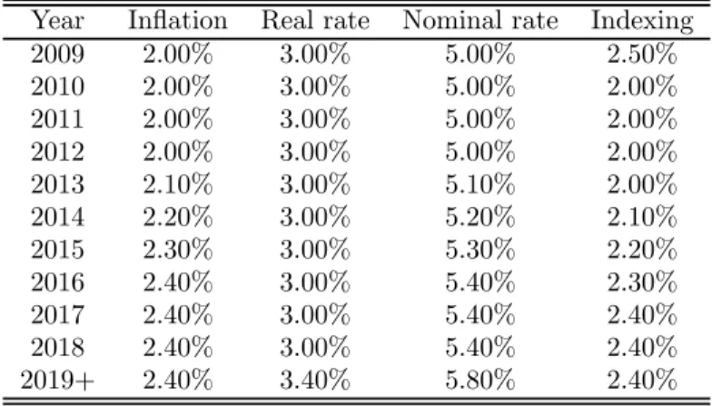
(18) 4. Applications. Given that actuarial reports for the Royal Canadian Mountain Police (RCMP) and the Canadian Forces (CF) are publicly available, we will now apply the CBD model to measure the longevity risk of the two defined benefit pension plans. The benefit corresponds to a percentage of the employee’s salary multiplied by the number of years of pensionable service. Since payments are set in advance, it is crucial to determine the number of future payments (i.e., the number of years the pensioners is expected to live). We will calculate the actuarial liability using two methods: The Office of the Chief Actuary (OCA) method as well as the CBD method. We will stress the difference between the two by calculating the ratio of CBD to OCA. A ratio greater than one implies that the CBD model predicts higher survival rates. Economic and demographic hypotheses are taken from the OCA’s report. Table 1 depicts the nominal rates and indexing adjustments used to calculate the actuarial value of pensions. Year 2009 2010 2011 2012 2013 2014 2015 2016 2017 2018 2019+. Inflation 2.00% 2.00% 2.00% 2.00% 2.10% 2.20% 2.30% 2.40% 2.40% 2.40% 2.40%. Real rate Nominal rate 3.00% 5.00% 3.00% 5.00% 3.00% 5.00% 3.00% 5.00% 3.00% 5.10% 3.00% 5.20% 3.00% 5.30% 3.00% 5.40% 3.00% 5.40% 3.00% 5.40% 3.40% 5.80% Table 1. Indexing 2.50% 2.00% 2.00% 2.00% 2.00% 2.10% 2.20% 2.30% 2.40% 2.40% 2.40%. Table 2 shows the initial and ultimate plan year mortality reductions (%). For the CBD model, we fitted a least-squares line through the natural logarithms of the projected central death rates. The average annual rates of improvement were then obtained by taking the complement of the exponential of the slope. To be consistent OCA assumptions, the model was calibrated using data from 1989 to 2006. The gap between mortality rates for men and women is diminishing so that Canadian men should experience higher improvement rates than Canadian women over the next decades,as displayed in Table 2. The difference between the OCA and the CBD models lies in the way in which mortality rates evolve through time. In the OCA model, mortality reductions between 2009 and 2029 were obtained using linear interpolation; hence rates of improvements are constantly diminishing during this period.. 17.

(19) Age 45 50 55 60 65 70 75 80 85 90 95 100 105. Males OCA 2009 2029+ 1.75 0.70 1.86 0.70 2.05 0.70 2.24 0.70 2.43 0.70 2.35 0.70 2.10 0.70 1.70 0.70 1.05 0.64 0.60 0.40 0.20 0.40 0.00 0.40 0.00 0.40. CBD 2009+ 2.85 2.67 2.49 2.31 2.13 1.95 1.76 1.57 1.38 1.17 0.96 0.75 0.53 Table 2. Females OCA 2009 2029+ 1.40 0.70 1.46 0.70 1.40 0.70 1.34 0.70 1.28 0.70 1.25 0.70 1.25 0.70 1.10 0.70 0.70 0.64 0.35 0.40 0.10 0.40 0.00 0.40 0.00 0.40. CBD 2009+ 1.98 1.84 1.71 1.57 1.44 1.30 1.16 1.02 0.87 0.73 0.57 0.42 0.27. Although mortality improvements used in our calculations are the same as the overall Canadian population, mortality rates are relatively lower. Fortunately, the actuarial reports of the two cases we will study, the Royal Canadian Mounted Police and the Canadian Armed Forces, present assumed mortality rates for 2009 of individuals aged between 30 and 110. These are shown in Table 3.. Age 30 40 50 60 70 80 90 100 110. RCMP Regular members Male Female 0.0006 0.0003 0.0010 0.0006 0.0020 0.0010 0.0051 0.0032 0.0156 0.0100 0.0534 0.0295 0.1478 0.0942 0.2829 0.2304 0.5000 0.5000 Table 3. Canadian Forces Male Officer Other rank 0.0005 0.0008 0.0006 0.0009 0.0013 0.0027 0.0039 0.0091 0.0152 0.0261 0.0588 0.0691 0.1487 0.1567 0.3151 0.3286 0.5000 0.5000. Mortality rates are given only for successive 10-year intervals of age. To find intermediate ages we used cubic spline interpolation. We then transformed mortality rates into central death rates and backed-out the values to 2008 by applying the following relation. mx (t) =. mx (t + 1) 1 − ix (t). 18. (7).

(20) where ix (t) corresponds to the improvement in mortality for a person aged x at time t. Finally, starting in 2008, we applied mortality reductions to the central death rates for the remaining of the time span using both the OCA and the CBD models.. 4.1. Royal Canadian Mounted Police. Before estimating the actuarial liability of the RCMP’s pension plan, we offer a brief description of its members. RCMP’s workforce is divided into two categories: Regular and civilian members. Regular members account for the majority of the personnel. Of the 15, 505 pensioners, 94% are men and 88% are former regular members. In terms of contributors, there are 15, 990 (75%) men and 5, 222 (25%) women. Since the RCMP is male-dominated, longevity risk is essentially independent of the evolution of female mortality rates. Finally, 84% of contributors are regular members (17, 862) and 16% are civilian members (3, 350). Table 4 presents the RCMP’s pension plan’s balance sheet in millions of dollars for 2005 and 2008. Balance sheet ($ millions), Pension Plan of the Royal Canadian Mounted Police As at 31 March 2008 As at 31 March 2005 Actuarial value of assets 14, 823 12, 284 Actuarial liability Regular members - Contributors - Retirement pensioners - Disability pensioners - Surviving dependants. 14, 301. 11, 382. 5, 737 6, 393 623 315. 4, 996 4, 823 365 232. Civilian members - Contributors - Retirement pensioners - Disability pensioners - Surviving dependants Administrative expenses. 627 411 63 22 110. 542 282 43 20 79. Actuarial surplus / (deficit). 522. 902. Table 4 The plan’s total actuarial liability is equal to 14, 301 millions of dollars. The present value of pensions paid to the current retirees represents 48% of this total, whereas another 45% includes the present value of future payable benefits to contributors that are not yet in payment. The remainder of the actuarial liability is ascribable to the pensions offered to pensioners with a disability and surviving dependants. We also note from the balance sheet that pension promises made to regular member (pensioners and contributors) account for 85% of the actuarial liability. Consequently, we shall concentrate our analysis on this subgroup. 19.

(21) 4.1.1. Retirement pensioners. Even if we concentrate only on regular members, the actuarial report does not contain all the information we need to evaluate the actuarial liability so we must make a few assumptions. For instance, we use the median age for each quinquennial age groups. In addition, we must assume that each year a pensioner receives an amount equal to the average annual pension of its age group. Finally, we do not include values for ages below 45 and above 84 since they represent only 2% of the pensioners. Results are shown in Table 5. Age 45 − 49 50 − 54 55 − 59 60 − 64 65 − 69 70 − 74 75 − 79 80 − 84 Total. Ratio (CBD/OCA) 1.0184 1.0170 1.0153 1.0139 1.0135 1.0143 1.0163 1.0186 1.0150. Male Liability ($ millions) 163.40 834.39 1, 908.81 1, 641.41 798.32 434.96 208.28 19.50 6, 009.07. % retired 2.660 13.583 31.074 26.721 12.996 7.081 3.391 0.317 97.824 Table 5. Ratio (CBD/OCA) 1.0062 1.0060 1.0057 1.0057 1.0061 1.0073 − 1.0106 1.0060. Female Liability ($ millions) 37.25 54.87 31.37 9.42 0.42 0.28 − 0.07 133.68. % retired 0.606 0.893 0.511 0.153 0.007 0.005 − 0.001 2.176. Total liabilities ascribable to regular members are equal to 6,393 million dollars according to the RCMP’s balance sheet. In table 5, our calculations give us a total liability for regular members of 6,143 million dollars. The difference between the two values comes from the fact that we were unable to reconstitute perfectly the calculations (because we use the median age rather than the actual age of the members). The difference is small, however, and should only have a marginal impact on the measure of longevity risk. Compared to the OCA model, the CBD model predicts on average higher diminution in mortality rates, hence the ratio of actuarial liabilities is always greater than one. Furthermore, the discrepancy is lower for intermediate ages. In fact, the difference is 1.84% for members aged 45 to 49 and 1.86% for members aged 80 to 84. In contrast, the difference is only 1.35% for members in the age group of 65 to 69. Luckily, intermediate ages constitute the majority of actuarial liability, so the total difference is attenuated to 1.50%. At last, the disparity is much lower for females, ranging from 0.57% to 1.06%. Consequently, females have almost no impact on the plan’s solvency, since males account for 97.82% of actuarial liability. The above evaluation is accomplished using the most probable trajectory of mortality rates. Longevity risk represents a departure from this trajectory. To demonstrate how sensitive the present value of future payments is to projected mortality rates, we calculated the relative and nominal Value-at-Risk at the 95th and 99th level. This risk measure is defined as the maximum expected loss in case of an adverse deviation 20.

(22) in the evolution of mortality rates. All values are presented in Table 6.. Age 45 − 49 50 − 54 55 − 59 60 − 64 65 − 69 70 − 74 75 − 79 80 − 84. Relative Value-at-Risk Male Female VaR VaR VaR VaR (95%) (99%) (95%) (99%) 2.39 3.59 0.69 1.02 2.58 3.89 0.75 1.10 2.75 4.17 0.80 1.18 2.90 4.41 0.85 1.25 3.01 4.59 0.89 1.31 3.06 4.67 0.92 1.36 3.04 4.65 − − 2.93 4.48 0.92 1.37 Table 6A. Nominal Value-at-Risk ($ millions) Male Female VaR VaR VaR VaR (95%) (99%) (95%) (99%) 3.977 5.966 0.260 0.383 21.878 32.992 0.413 0.609 53.339 80.781 0.252 0.372 48.274 73.375 0.080 0.119 24.346 37.114 0.004 0.006 13.504 20.622 0.003 0.004 6.435 9.833 − − 0.583 0.891 0.001 0.001 Table 6B. As shown in a previous section, there is a positive correlation between the longevity risk premium and the age of the policyholder. Hence, it is normal that we obtain higher values-at-risk for older age cohorts. Moreover, we notice that for both genders and for all levels of confidence, the relative VaR increases continually until it reaches a peak in the age bracket 70 to 74, and then decreases. Since there is a small probability that a pensioner aged 75 and older lives much longer than predicted, the VaR is relatively smaller for those ages. In terms of dollars, the VaR is remarkably superior for members for whom the actuarial liability is highest; in our case, members aged 50 to 59. Finally, because longevity risk is mainly driven by males, their relative and nominal values-at-risk are always greater than those of females. 4.1.2. Contributors. To determine actuarial liability with respect to contributors we must determine the amount of future payments based on current annual earnings. For calculation purposes we take the median age of each group, the median year of pensionable service and average pensionable earnings. Also, to simplify matter, we assume that a member that has less than 20 years of service receives a deferred annuity that starts being effective at age 60. A member that retires after 20 to 24 years of service is given an annual allowance. And a member with more than 25 years of service collects an immediate annuity. All types of benefits are indexed in the first year following retirement. The annual amount received is equal to 2% of the average pensionable earnings multiplied by number of credited service under the plan. Starting at age 65, the annual pension amount is reduced by a percentage of the indexed Canadian Pension Plan (CPP) annual pensionable earnings multiplied by the years of CPP pensionable service. In our evaluation all contributors will reach age 65 in 2012 or later, hence in all cases the. 21.

(23) appropriate reduction factor will be 0.625 per cent as we see in Table 7 Panel A. Furthermore, as presented in Table 7 Panel B, in the case of an annual allowance, payments are further reduced by 5% for each year by which pensionable service is less than 25 or by which the age at retirement is less than 60 (the lesser of the two). For example, omitting any pension increases due to indexing, a regular male member that retires in 2008 at age 42 with 22 years of pensionable service receives $34, 162 in annual allowances until he reaches the age of 65 at which point he receives $28, 324.. Coordination percentage. Calendar years 2008 2009 2010 2011 0.685% 0.670% 0.655% 0.640% Table 7A. Age at departure Average salary Years of pensionable service Pension that would have been payable starting at age 60 Reduction Annual allowance payable from age 42 CPP/QPP integration reduction Annual allowance payable from age 65 Table 7B. 2012+ 0.625%. 42 years old $91, 343 22 2% × 22 × $91, 343 = $40, 191 5% × (25 − 22) × $40, 191 = $6, 029 $40, 191 − $6, 029 = $34, 162 0.625% × 22 × $42, 460 = $5, 838 $34, 162 − $5, 838 = $28, 324. The Table 8 results were obtained, where (d) refers to the case of a deferred annuity and (i) refers to that of an immediate annuity. We observe once again larger ratios for males than for females; but most interestingly, we notice that the ratios are greater for contributors than for pensioners. Since the time span is much longer for contributors, it is not surprising that dissimilarities among the models in forecasted mortality, and consequently in actuarial values, are accentuated. Moreover, for both types of annuities the ratio becomes closer to one as the pensioners gets older. The OCA model relies on the assumption that mortality rates decrease at a diminishing rate whereas the CBD model presumes that mortality rates decrease continually. On that account, the divergence in actuarial values is highlighted at younger ages because the projection period is longer. It is even more important for differed annuities considering that payments start only at age 60. For example, given a policyholder under 25 years of age, the dissimilarity between the two models is as great as 6.49% for males and 6.16% for females. However, the discrepancy diminishes with age. In total, under the CBD model, actuarial liability is 2.07% higher for males and only. 22.

(24) 0.86% higher for females.. Age −25 (d) 25 − 29 (d) 30 − 34 (d) 35 − 39 (d) 40 − 44 (d) 40 − 44 (i) 45 − 49 (d) 45 − 49 (i) 50 − 54 (d) 50 − 54 (i) 55 + (d) 55 + (i) Total. Ratio (CBD/OCA) 1.0649 1.0634 1.0570 1.0499 1.0420 1.0169 1.0335 1.0166 1.0250 1.0157 1.0202 1.0149 1.0207. Male Liability (million $) 5.85 32.34 89.37 209.30 325.90 360.96 148.45 1, 387.57 48.56 1, 691.61 13.00 812.12 5, 125.02. % retired 0.100 0.551 1.524 3.569 5.558 6.156 2.531 23.662 0.828 28.847 0.222 13.849 87.397 Table 8. Ratio (CBD/OCA) 1.0186 1.0182 1.0167 1.0149 1.0129 1.0055 1.0107 1.0056 1.0085 1.0055 1.0073 1.0055 1.0086. Female Liability (million $) 1.95 13.78 41.43 84.53 86.23 123.84 25.37 210.68 10.78 114.10 3.01 23.34 739.04. % retired 0.033 0.235 0.706 1.442 1.470 2.112 0.433 3.593 0.184 1.946 0.051 0.398 12.603. Lastly, we calculate the relative and nominal VaRs. We distinguish between immediate and deferred annuities on the basis that they exhibit different levels of risk. Results are detailed in Tables 9.. Age −25 (d) 25 − 29 (d) 30 − 34 (d) 35 − 39 (d) 40 − 44 (d) 40 − 44 (i) 45 − 49 (d) 45 − 49 (i) 50 − 54 (d) 50 − 54 (i) 55 + (d) 55 + (i). Relative Value-at-Risk Male Female VaR VaR VaR VaR (95%) (99%) (95%) (99%) 6.25 9.10 1.83 2.68 6.20 9.06 1.80 2.64 5.85 8.62 1.68 2.47 5.43 8.06 1.54 2.27 4.95 7.40 1.40 2.06 1.93 2.87 0.56 0.83 4.40 6.61 1.24 1.83 2.16 3.24 0.62 0.92 3.79 5.72 1.08 1.59 2.38 3.58 0.69 1.01 3.39 5.12 0.97 1.43 2.50 3.78 0.73 1.07 Table 9A. Dollar Value-at-Risk ($ million) Male Female VaR VaR VaR VaR (95%) (99%) (95%) (99%) 0.390 0.567 0.036 0.053 2.132 3.116 0.252 0.371 5.525 8.138 0.706 1.038 11.937 17.710 1.322 1.946 16.820 25.115 1.220 1.797 7.077 10.552 0.699 1.029 6.756 10.145 0.318 0.469 30.427 45.644 1.321 1.946 1.886 2.846 0.117 0.172 40.810 61.539 0.786 1.159 0.449 0.679 0.030 0.044 20.622 31.180 0.171 0.252 Table 9B. As demonstrated earlier, the longer the time horizon, the less precision the model offers. Henceforth it is harder to predict future mortality rates for younger cohorts since the forecasting period is longer. This is illustrated by a decreasing relative value-at-risk with age. The dollar VaR is greater for the age brackets where policyholders are mostly concentrated.. 23.

(25) 4.2. Canadian Forces. To further emphasize on the impact the choice of a forecasting model has on actuarial liability, we repeat our methodology using the Canadian Forces’ pension plan. However, since all tables unveil the same characteristics, we only compare the magnitude of the longevity risk faced by both the RCMP and the Canadian Forces. For the RCMP we considered regular members of both genders. Because the institution consists mainly of men; we showed that females do not have a great impact on actuarial premiums. The Canadian Forces is even more homogeneous, that is to say, 95% of pensioners and 85% of contributors are males. For instance, there are 70, 480 male as opposed to 3, 396 female pensioners, and 57, 573 male to 9, 869 female contributors. Since females will have almost no impact on actuarial liability, we decided to exclude them from our evaluation of the Canadian Forces pension plan and only consider the two main classes of employees: male officers and males of other ranks. Finally, because 94% of actuarial liability is imputable to active contributors and retirement pensioners, we omit all other classes in our evaluation. Table 10 details the plan’s financial situation. Balance sheet ($ millions), Pension Plan of the Canadian Armed Forces As at 31 March 2008 As at 31 March 2005 Actuarial value of assets 52, 224 45, 383 Actuarial liability - Active contributors - Retirement pensioners - Disability pensioners - Surviving dependants - Administrative expenses Actuarial surplus / (deficit). 50, 532 16, 246 31, 127 379 2, 626 154. 42, 701 14, 565 25, 301 385 2, 275 175. 1, 692. 2, 682. Table 10 The Canadian Forces’ actuarial liability is much higher than the RCMP’s; it amounts to 50, 532 millions of dollars. Notwithstanding, apart from the nominal values-at-risk, our results are independent of the principal; they are merely conditional upon the forecasted mortality rates. All information used in our calculations is presented in Appendix B. We included the number and average annual pension as at March 2008 for male retirement pensioners in addition to the number and average annual pensionable earnings for male contributors. The tables for the pensioners do not distinguish between officers and other ranks, so we assumed that they are represented in the same percentage in each quinquennial age as they are in the overall population, particularly, 23% officers and 77% other ranks. Interestingly, officers and other ranks are 24.

(26) represented in identical proportion among the male contributors. 4.2.1. Retirement pensioners. To be consistent with our assumptions made in the RCMP’s evaluation, we considered exclusively pension with indexing and we did not include values for ages above 84. Note that there are no pensions offered to policyholder under 55 years of age. Results are shown in Table 11. Age 55 − 59 60 − 64 65 − 69 70 − 74 75 − 79 80 − 84 Total. Ratio (CBD/OCA) 1.0152 1.0136 1.0128 1.0135 1.0157 1.0180 1.0140. Officers Liability ($ millions) 536.86 1, 095.16 1, 024.37 718.39 422.40 180.20 3, 977.39. % retired 3.352 6.837 6.395 4.485 2.637 1.125 24.831 Table 11. Ratio (CBD/OCA) 1.0118 1.0091 1.0080 1.0089 1.0114 1.0140 1.0096. Other ranks Liability ($ millions) 1, 630.85 3, 293.19 3, 075.36 2, 176.75 1, 300.40 563.75 12, 040.29. % retired 10.182 20.560 19.200 13.590 8.119 3.520 75.169. When calculating the ratio of CBD to OCA we cancel all periodic payments and we are left with an annuity factor (present value of a stream that provides one unit each period). Accordingly, the discrepancy between the two actuarial values is entirely attributable to differences in mortality forecasting among the models. Attesting this conjecture, we compare the results of the RCMP’s males and the Canadian Forces’ male officers. Both groups have essentially the same mortality rates as at 2008; they should consequently have similar ratios. This is exactly what is observed. Finally, there appears to be a negative relation between the ratios and the initial mortality rates. Since our model predicts better longevity improvements than the OCA model, the difference between the two models becomes larger as the time horizon increases. Hence, the greater chance of survival in the far future, the higher the ratios. Consequently, it is not surprising that the group that has the highest mortality rates, specifically Canadian Forces’ males of other ranks, has the lowest percentages. Table 12 presents the relative and nominal values-at-risk of the Canadian Forces.. Age 55 − 59 60 − 64 65 − 69 70 − 74 75 − 79 80 − 84. Relative Value-at-Risk Officers Other ranks VaR VaR VaR VaR (95%) (99%) (95%) (99%) 2.72 4.13 3.14 4.60 2.87 4.37 3.27 4.81 2.98 4.54 3.35 4.94 3.02 4.61 3.37 4.98 2.98 4.55 3.31 4.88 2.84 4.35 3.16 4.66 Table 12A 25. Dollar Value-at-Risk ($ millions) Officers Other ranks VaR VaR VaR VaR (95%) (99%) (95%) (99%) 14.829 22.515 51.746 75.985 31.867 48.525 108.596 159.832 30.895 47.154 103.948 153.250 21.980 33.596 74.096 109.269 12.766 19.524 43.578 64.203 5.218 7.983 18.089 26.616 Table 12B.

(27) As expected, the RCMP’s males and the Canadian Forces’ male officers have analogous relative valuesat-risk. Moreover, we notice that the percentages are lowest for the RCMP’s females and highest for the Canadian Forces’ males of other ranks. Since any deviation from the expected trajectory is heightened at higher central death rates; the relative VaRs are positively correlated to the initial mortality rates. Figure 6 illustrates graphically our results. Note that RCMP females have lower relative VaRs since they have comparatively lower mortality rates and inferior longevity improvements. Relative Value-at-Risk at the 90th level for the RCMP and Canadian Forces pensioners 0.03. Relative VaR (%). 0.025. 0.02. 0.015. RCMP males RCMP females CF male officers CF males of other ranks. 0.01. 0.005 55. 60. 65. 70 Age. 75. 80. 85. Figure 6 Ultimately, we observe that the amount of actuarial liability only affects the nominal VaR. In addition, since other ranks are more numerous than officers their nominal values-at-risk are always greater. 4.2.2. Contributors. The calculations are essentially the same as for the RCMP,. For members with less than 20 years of service, a deferred annuity at age 60 is provided and for members with more than 20 years of service an immediate annuity is offered. Results are shown in Table 13. At the risk of sounding repetitive, we observe comparable values for members that have homologous mortality rates even though their pension differs. We also notice that for immediate annuities the ratios are higher for groups that have lower initial mortality rates. The opposite is observed for deferred annuities. For instance, for a policyholder aged 25 years of age, we must predict mortality rates for another 35 years before calculating the annuity. Since longevity improvements are higher for the CBD model, mortality rates at age 60 are much lower than the ones predicted by the OCA. For that reason, the ratios are largest for the Canadian Forces’ males of other ranks. For example, the difference between the CBD and OCA is as high as 7.07% for members of other ranks aged 25 to 29, but 26.

(28) only 6.21% for officers. Starting at age 45, the forecasting period is shorter; hence the impact of mortality reduction is lower. In that case, the results are comparable to the ones obtained for immediate annuities.. Age. Officers Liability (million $) 13.08 58.54 159.09 277.66 182.61 1, 245.93 73.90 1, 830.21 30.14 1, 192.26 8.31 255.19 5, 326.93. Ratio (CBD/OCA) 1.0624 1.0621 1.0564 1.0494 1.0417 1.0167 1.0335 1.0165 1.0252 1.0157 1.0204 1.0150 1.0210. −25 (d) 25 − 29 (d) 30 − 34 (d) 35 − 39 (d) 40 − 44 (d) 40 − 44 (i) 45 − 49 (d) 45 − 49 (i) 50 − 54 (d) 50 − 54 (i) 55 + (d) 55 + (i) Total. % retired 0.097 0.436 1.185 2.068 1.360 9.279 0.550 13.630 0.224 8.879 0.062 1.900 39.672 Table 13. Ratio (CBD/OCA) 1.0725 1.0707 1.0626 1.0535 1.0432 1.0171 1.0324 1.0157 1.0219 1.0134 1.0164 1.0118 1.0234. Other ranks Liability (million $) 57.61 171.17 293.07 668.01 303.26 2, 748.18 61.32 2, 699.94 12.48 959.01 3.05 123.32 8, 100.42. % retired 0.429 1.275 2.183 4.975 2.259 20.467 0.457 20.108 0.093 7.142 0.023 0.918 60.328. As seen from Figure 7, around age 55, pensioners have relatively higher ratios than contributors. As mentioned earlier, the ratio of CBD to OCA is equivalent to an annuity factor. For pensioners, since the average annual amount is already reduced by the CPP offset, the annuity generates a series of equal payments of one for all the projection period. In contrast, the amount disbursed to contributors must be lowered once the policyholder reaches age 65. In that event, the present value is comparatively smaller. Ratio of CBD to OCA for the RCMP and CF male members (immediate annuities). Ratio of CBD to OCA for the RCMP and CF male contributors (deferred annuities) 1.07. 1.018 Contributors. 1.017. 1.065 1.06. 1.016. 1.055 Pensioners. 1.014. CBD/OCA. CBD/OCA. 1.015. 1.013 1.012. 1.05 1.045 1.04 1.035. 1.011. 1.03 1.01. RCMP CF officers CF other ranks. 1.009 45. 50. 55. 1.025 1.02 60. 65. 70. 75. 80. 25. Age. Figure 7. RCMP CF officers CF other ranks 30. 35. 40 Age. 45. 50. 55. Figure 8. Finally, we display the relative and nominal values-at-risk. We observe once more in Table 14 that the. 27.

(29) relative VaRs are positively correlated to the initial mortality rates.. Age −25 (d) 25 − 29 (d) 30 − 34 (d) 35 − 39 (d) 40 − 44 (d) 40 − 44 (i) 45 − 49 (d) 45 − 49 (i) 50 − 54 (d) 50 − 54 (i) 55 + (d) 55 + (i). 5. Relative Value-at-Risk Officers Other VaR VaR VaR (95%) (99%) (95%) 6.13 8.98 7.60 6.18 9.08 7.55 5.87 8.69 7.08 5.44 8.11 6.53 4.95 7.42 5.88 1.95 2.92 2.19 4.40 6.64 5.15 2.16 3.25 2.41 3.80 5.75 4.36 2.37 3.59 2.64 3.40 5.15 3.85 2.50 3.79 2.78 Table 14A. ranks VaR (99%) 10.81 10.78 10.18 9.44 8.55 3.18 7.52 3.52 6.38 3.87 5.65 4.08. Dollar Value-at-Risk ($ millions) Officers Other ranks VaR VaR VaR VaR (95%) (99%) (95%) (99%) 0.850 1.245 4.693 6.680 3.845 5.648 13.830 19.748 9.862 14.599 22.039 31.687 15.849 23.624 45.952 66.468 9.417 14.121 18.598 27.039 24.714 37.017 61.231 88.875 3.363 5.069 3.263 4.763 40.172 60.497 66.194 96.535 1.173 1.775 0.555 0.814 28.740 43.478 25.690 37.610 0.288 0.437 0.119 0.175 6.478 9.822 3.470 5.090 Table 14B. Conclusion. The goal of this paper was to present an assessment of the cost of longevity risk for two Canadian public pension plans: The Royal Canadian Mounted Police and the Canadian Armed Forces. Longevity risk is defined in our context as the risk that a pension plan will run out of funds before the last pensioner has died, not because of misappropriation of funds or bad investment, but because the life expectancy of the pensioner was under-estimated. In a broader context, longevity risk represents the risk that an organization (corporation, insurer) or an individual lives longer than the assets that were put aside. This risk is becoming more and more important in value as the general population in Canada, and in the developed as well as in the developing world, is living longer upon retirement. The specificity of this risk is that is cannot be diversified through the law of large numbers since it represents a macro risk. The current paper compares two models to forecast longevity. There are, of course, a much larger set of models in the academic literature that attempt to achieve such forecasts. These would undoubtedly offer predictions that would differ from we presented. Nonetheless, using a portfolio of model approach highlights the risk inherent to the difficulty of predicting long-term longevity. Managing appropriately the longevity risk (and funding it accordingly) should attract the attention of both sponsors and authorities to fully apprehend the scope of the underlying uncertainty. No model can be said to replicate the trends of mortality through time, but plans can incorporate additional reserves to compensate for this risk. This is what we did. Using. 28.

(30) a simulation method of future mortality, we calculated the necessary reserves that would ensure, with 95% or 99% certainty, that the fund will not run out of money because of an underestimation of the mortality If the projections we made using a Lee-Carter model of an Cairns-Blake-Dowd (CBD) model turn out to be correct, the longevity risk faced by the pension plans of both the RCMP and Canadian Forces is substantial. Our model may even be too optimistic in the sense that stochastic mortality trends are overestimated even with these two model. The reason is that both models assume implicitly that longevity improvements will be continuous, even in the far future. If on the other hand future mortality trends vary by leaps and bounds rather than continuously, our forecast over-estimates future mortality, which means that current plan sponsors are under-reserving for future longevity risk shocks. There are different views on how future mortality rates may evolve through time. Some pretend that there is a biological limit to life while others predict that mankind can achieve physical immortality. Since scientists disagree on the limit of longevity, selecting a forecasting model is a subjective process. In this regard, there is no clear way of knowing whether the CBD model is adequate and superior to the OCA. Actually, the purpose of this paper is not to claim that one predictive model is more appropriate than the other, but rather to highlight the impact the choice of model can have on the solvency ratio of a defined benefit pension plan. By comparing the assumptions made by the Office of the Chief Actuary with those of the CBD model, we can clearly ascertain that there is a significant divergence in the present value of future benefits for both the RCMP and the Canadian Forces plans. These differences can eventually imply several hundreds of millions of dollars in either additional contributions or in surplus. Both cases can imply negative consequences for the promoter of the plan.. 29.

(31) 6. References 1. Antolin, P. (2007). Longevity Risk and Private Pensions. OECD Working Paper on Insurance and Private Pensions, 2007. 2. Boucher, P. and M.M. Boyer (2010). Le risque de longévité: une application au régime de retraite de la Gendarmerie royale du Canada. Assurances et gestion des risques, 78(3). 3. Boucher, P. and M.M. Boyer (2009). Le risque de longévité: valorisation et outils de gestion. Assurances et gestion des risques, 77(3). 4. Cairns, A. J. G., D. Blake, and K. Dowd (2006). A Two-Factor Model for Stochastic Mortality with Parameter Uncertainty: Theory and Calibration. Journal of Risk and Insurance, 73(4): 687—718. 5. Canada Pension Plan, Mortality Study, July 2009, Office of the Chief Actuary, Actuarial Study no.7. 6. Canadian Forces - Regular Forces, Actuarial Report on the Pension Plan for the Canadian Forces as at 31 March 2008, Office of the Chief Actuary. 7. Dowd, K, A.J.G. Cairns and D. Blake (2010). Facing Up to Uncertain Life Expectancy: the Longevity Fan Charts. Demography, 47(1). 8. Dowd, K, A.J.G. Cairns, D. Blake, G.D. Coughlan, D.Epstein and M. Khalaf-Allah (2009). Backtesting Stochastic Mortality Models: an Ex-Post Evaluation of Multiperiod-Ahead Density Forecast. North American Actuarial Journal, 14(3). 9. Friedberg, L., and A. Webb (2007). Life Is Cheap: Using Mortality Bonds to Hedge Aggregate Mortality Risk. The B.E. Journal of Economic Analysis & Policy, 7:1—31.. 10. Fujisawa, Y., and J. S.-H. Li (2010). IFRS Convergence: The Role of Stochastic Mortality Models in the Disclosure of Longevity Risk for Defined Benefit Plans. Asia-Pacific Journal of Risk and Insurance, 5:1—25. 11. Human Mortality Database (2010). University of California at Berkeley, http://mortality.org/. 12. Lee, R.D., and L.R. Carter (1992). Modeling and Forecasting U.S. Mortality. Journal of the American Statistical Association, 87(419):659—671.. 30.

(32) 13. Milevsky, M., S. D. Promislow, and V. R. Young (2006). Killing the Law of Large Numbers: Mortality Risk Premium and the Sharpe Ratio. Journal of Risk and Insurance, 73(4): 673—686. 14. Public Service Death Benefit Account, Actuarial Report on the Public Service Death Benefit Account as at 31 March 2008, Office of the Chief Actuary. 15. Renshaw, A., and S. Haberman (2006). A Cohort-based Extension to the Lee-Carter Model for Mortality Reduction Factors. Insurance: Mathematics and Economics, 38(419): 556—570. 16. Royal Canadian Mounted Police, Actuarial Report on the Pension Plan for the Royal Canadian Mounted Police as at 31 March 2008, Office of the Chief Actuary. 17. Olshansky, S.J., B.A. Carnes, M.S. Mandell (2009). Future Trends in Human Longevity: Implications for Investments, Pensions and the Global Economy. Pensions 2009.. 31.

(33)