HAL Id: tel-02052844
https://tel.archives-ouvertes.fr/tel-02052844
Submitted on 28 Feb 2019HAL is a multi-disciplinary open access archive for the deposit and dissemination of sci-entific research documents, whether they are pub-lished or not. The documents may come from teaching and research institutions in France or
L’archive ouverte pluridisciplinaire HAL, est destinée au dépôt et à la diffusion de documents scientifiques de niveau recherche, publiés ou non, émanant des établissements d’enseignement et de recherche français ou étrangers, des laboratoires
Confident alternate test implementation
Syhem Larguech
To cite this version:
Syhem Larguech. Confident alternate test implementation. Micro and nanotechnolo-gies/Microelectronics. Université Montpellier, 2015. English. �NNT : 2015MONTS185�. �tel-02052844�
Préparée au sein de l’école doctorale
I2S
Et de l’unité de recherche
LIRMM/UMR 5506
Spécialité:
Systèmes Automatiques et Microélectroniques (SYAM)Présentée par
Syhem Larguech
Test indirect des circuits analogiques et
RF: Implémentation sûre et efficace
***
Confident alternate test implementation
Soutenue le 03-12-2015 devant le jury composé de
Dr. Serge Bernard CR CNRS-LIRMM Invité
(Directeur de thèse )
Dr. Florence Azais CR CNRS-LIRMM Invitée
(Co-directrice de thèse)
Dr. Haralampos Stratigopoulos CR CNRS-LIP6 Rapporteur
Dr. Gildas Léger CR CSIC-IMSE Rapporteur
Dr. Michel Renovell DR CNRS-LIRMM Examinateur
Dr. Laurent Latorre Pr Univ. Montpellier Examinateur
Dr. Emmanuel Simeu Mdc Univ. Grenoble Invité
Dr. Manuel Barragan CR CNRS-TIMA Invité
Dr. François Lefèvre Ing NXP Semiconductors Invité
Dr. Mariane Comte Mdc Univ. Montpellier Invitée
I would like to thank Dr. Haralampos Stragopoulos, Dr. Gildas Leger, Dr. Emmanuel Simeu, Dr. Manuel Barragan, Dr. Michel Renovell, Dr. Laurent Latorre and Mr. François lefèvre for their implication. It is a pleasure and honor that they accepted to be part of my dissertation committee.
Acknowledge- ment goes to
the best team ever ♥ F. Azais, S. Bernard, V.
Kerzerho, M. Comte and M. Renovell ♥ for supporting my thesis. I really enjoyed the work with them and learned a lot from each one of them. I am lucky to have many advisors by my side providing me with an excellent guidance and atmosphere for the research. I m deeply grateful to ♥ Florence who has always been present and effectively supporting this thesis; her valuable suggestions and writing skills have made many publications possible. ♥ Serge has always been supporting and encouraging me. I also want to greet his sense of humanity that keeps me feeling that he is a friend of mine. ♥ Vincent has been actively participating in this work. I want to thank him a lot. ♥ Mariane
is the first one to believe in me since my masters till my thesis project. I thank her for her support, kindness and attitude. ♥ Michel is always with a smiling
face, giving me energy and happiness. I want to thank him for his support and care. Also, I would like to thank all the♥ LIRMM ♥ community and
above all Arnaud Virazel and Pascal Nouet for hosting and supporting me during these 4 years. I m thankful to ♥ my collegues and♥ dear
freinds Anu, Patcharee, Mohamed, Aymen, Alejandro, Stephane ... for the love, care and happiness that they give me.
Finally, I m thankful to ♥ my father, my two broth-ers, my aunt, my grand mothers and my uncles
who are always supporting me wherever I am in need. This work is
dedi-cated to the memory of my mother, ♥ and all
of you! ♥
eing able to check whether an IC is fully functional or not after the manufacturing process, is very difficult. Particularly for analog and Radio Frequency (RF) circuits, test equipment and procedures required have a major impact on the circuits cost. An interesting approach to reduce the impact of the test cost is to measure parameters requiring low-cost test resources and correlate these measurements, called indirect measurements, with the targeted specifications. This is known as alternate or indirect test technique because there is no direct measurement for these specifications, which requires so expensive test equipment and an important testing time, but these specifications are estimated w.r.t "low-cost measure-ments". While this approach seems attractive, it is only viable if we are able to establish a sufficient accuracy for the performance estimation and if this estimation remains stable and independent from the circuits sets under test.
The main goal of this thesis is to implement a robust and effective indirect test strategy for a given application and to improve test decisions based on data analysis.
To be able to build this strategy, we have brought various contributions. Initially, we have defined new metric developed in this thesis to assess the reliability of the estimated perfor-mances. Secondly, we have analyzed and defined a strategy for the construction of an optimal model. This latter includes a data preprocessing followed by a comparative analysis of dif-ferent methods of indirect measurement selection. Then, we have proposed a strategy for a confident exploration of the indirect measurement space in order to build several best models that can be used later to solve trust and optimization issues. Comparative studies were per-formed on two experimental data sets by using both of the conventional and the developed metrics to evaluate the robustness of each solution in an objective way.
Finally, we have developed a comprehensive strategy based on an efficient implementation of the redundancy techniques w.r.t to the build models. This strategy has greatly improved the robustness and the effectiveness of the decision plan based on the obtained measurements. This strategy is adaptable to any context in terms of compromise between the test cost, the confidence level and the expected precision.
More generally, this study constitutes an overview to guide the test engineer regarding prac-tical aspects of alternate test implementation.
Key words: Alternate test, indirect test, analog/RF ICs, data mining, machine learning, statistical techniques, correlation and modeling.
tre en mesure de vérifier si un circuit intégré est fonctionnel après fabrication peut s´avérer très difficile. Dans le cas des circuits analogiques et Radio Fréquence (RF), les procédures et les équipements de test nécessaires ont un impact majeur sur le prix de revient des circuits. Une approche intéressante pour réduire l´impact du coût du test consiste à mesurer des paramètres nécessitant des ressources de test faible coût et corréler ces mesures, dites mesures indirectes, avec les spécifications à tester. On parle alors de technique de test indirect (où test alternatif) car il n´y a pas de mesure directe des spécifications, qui nécessit-erait des équipements et du temps de test importants, mais ces spécifications sont estimées à partir des mesures "faibles coûts". Même si cette approche semble attractive elle n´est fiable que si nous sommes en mesure d´établir une précision suffisante de l´estimation des performances et que cette estimation reste stable et indépendante des lots de circuits à traiter. L´objectif principal de cette thèse est de mettre en œuvre une stratégie générique permettant de proposer un flot de test indirect efficace et robuste. Pour être en mesure de construire cette stratégie nous avons apporté différentes contributions. Dans un premier temps, on a développé une nouvelle métrique pour évaluer la robustesse des paramètres estimés. Dans un deuxième temps, on a défini et analysé une stratégie pour la construction d´un modèle optimal. Cette dernière contribution englobe un prétraitement de données puis une analyse comparative entre différentes méthodes de sélections de mesures indirectes ainsi que l´étude d´autres paramètres tels que la taille des combinaisons de mesures indirectes ainsi que la taille du lot d´apprentissage. Nous avons également proposé une stratégie d´exploration de l´espace des mesures indirectes afin de construire plusieurs modèles précis nécessaires pour résoudre les problèmes de précision et de confiance dans les estimations. Les études com-paratives réalisées ont été effectuées sur deux cas d´études expérimentaux, en utilisant des métriques classiques ainsi qu´une nouvelle métrique permettant d´évaluer objectivement la robustesse de chaque solution.
Enfin, nous avons développé une stratégie complète mettant en œuvre des techniques de re-dondance de modèles de corrélation qui permettent d´améliorer clairement la robustesse et l´efficacité de la prise de décision en fonction des mesures obtenues. Cette stratégie est adapt-able à n´importe quel contexte en termes de compromis entre le coût du test et les niveaux de confiance et de précision attendus.
Mots clés: Test alternatif, test indirect, circuits analogiques et Radio Fréquence, traitement de données, algorithme d´apprentissage, analyse statistique, modélisation, corrélation.
Acknowledgements i
Abstract iii
Résumé v
List of Figures ix
List of Tables xiii
Introduction 1
1 Alternate test and data mining 3
1.1 Some principles of data mining . . . 4
1.1.1 KDD Process . . . 5
1.1.2 Machine-learning Algorithms . . . 6
1.2 Indirect test . . . 9
1.2.1 Introduction . . . 9
1.2.2 Classification-oriented indirect test . . . 10
1.2.3 Prediction-oriented indirect test . . . 10
1.3 Prediction-oriented indirect test strategy . . . 11
1.3.1 Training phase . . . 13
1.3.2 Validation phase . . . 13
1.3.3 Production testing phase . . . 13
1.3.4 Problematic . . . 14
1.4 Metrics for test efficiency evaluation . . . 14
1.4.1 Accuracy metrics . . . 15
1.4.2 Prediction reliability: Failing Prediction Rate (FPR) . . . 16
1.5 Choice of the regression algorithm . . . 18
1.6 Summary . . . 22
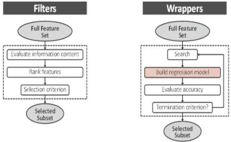
2 Single model approach: outlier filtering and selection of indirect measure-ments 23 2.1 Outlier filtering . . . 25
Contents
2.1.2 Adaptive k-filter . . . 26
2.2 Methods for indirect measurement selection . . . 30
2.2.1 IM selection based on Pearson correlation . . . 32
2.2.2 IM selection based on Brownian distance correlation . . . 33
2.2.3 IM selection based on SFS algorithm . . . 34
2.2.4 IM selection using MARS built-in selection feature . . . 36
2.3 Experimental setup for the evaluation of IM selection methods . . . 36
2.3.1 IMs selection . . . 37
2.3.2 Indirect test efficiency evaluation . . . 38
2.4 Results and discussion . . . 39
2.4.1 IM selection . . . 39
2.4.2 Test efficiency . . . 43
2.5 Summary . . . 51
3 Multi-model approach: Model generation 53 3.1 IM space reduction . . . 54
3.1.1 PCA-based reduction . . . 54
3.1.2 Pearson correlation-based reduction . . . 57
3.1.3 Iterative MARS-based reduction . . . 58
3.1.4 Preliminary evaluation of IM space reduction solutions . . . 61
3.2 Multi-model generation . . . 62
3.2.1 Extended SFS-Parental strategy . . . 62
3.2.2 Extended SFS-Non Parental strategy . . . 63
3.2.3 Computational effort . . . 64
3.3 Evaluation . . . 65
3.3.1 Model accuracy: evaluation on TS . . . 65
3.3.2 Built models evaluation on VS . . . 68
3.3.3 Further analysis and discussion . . . 74
3.4 Summary . . . 78
4 Multi-model approach: Models redundancy 79 4.1 Model redundancy principle . . . 80
4.2 Generic framework . . . 83
4.2.1 Overview . . . 83
4.2.2 Selection and construction of redundant models . . . 84
4.2.3 Tradeoff exploration: reliability vs. cost . . . 86
4.3 Results . . . 87
4.3.1 Selection and construction of redundant models . . . 87
4.3.2 Tradeoff between test cost and test reliability . . . 90
4.4 Summary . . . 94
Conclusion 95
Related publications a
1.1 KDD . . . 5
1.2 Machine-learning algorithms . . . 7
1.3 Classification-oriented testing . . . 10
1.4 Prediction-oriented testing . . . 11
1.5 Prediction-oriented alternate testing synopsis . . . 12
1.6 Example of estimated vs. actual RF performance on the TS . . . 16
1.7 Example of estimated vs. actual RF performance on the VS . . . 17
1.8 An example of Failing Prediction Rate (FPR) achieved with two different mod-els . . . 18
1.9 PA test vehicle . . . 19
1.10 RF transceiver test vehicle . . . 20
2.1 Database form representation as a table of individuals (ICk), attributes (IMi) and classes (Pj) . . . 24
2.2 Histogram distribution for an indirect measurement over the IC population showing outlier circuits . . . 25
2.3 Examples of IM distribution encountered in the database (transceiver test vehicle) 26 2.4 Adaptive k-filter . . . 28
2.5 Examples of IM distribution before (a) and after (b) the filtering process (transceiver test vehicle) . . . 29
2.6 Correlation coefficient and estimation errors before and after the filtering pro-cess (transceiver test vehicle) . . . 30
2.7 Correlation graph for a transceiver performance performed on training set (TS) 31 2.8 Curse of dimensionality issue in the context of indirect testing . . . 32
2.9 The two main categories of feature selection algorithms . . . 32
2.10 SFS search of an IM subset for prediction of one specification Pj . . . 35
2.11 Experimental setup for test efficiency evaluation . . . 37
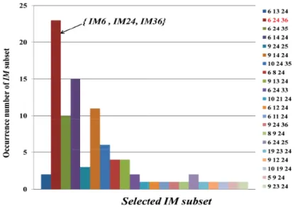
2.12 Illustration of chosen IM subsets over 100 runs (transceiver test vehicle) . . . . 38
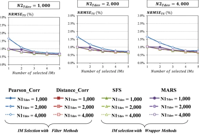
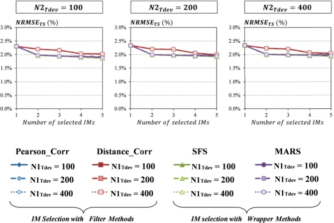
2.13 Model accuracy for the PA test vehicle considering different IM selection strate-gies and different sizes of training set (mean value over Nruns) . . . 44
2.14 Model accuracy for the transceiver test vehicle considering different IM selec-tion strategies and different sizes of training set (mean value over Nruns) . . . 45
2.15 Prediction accuracy for the PA test vehicle considering different IM selection strategies and different sizes of training set . . . 46
List of Figures
2.16 Prediction accuracy for the transceiver test vehicle considering different IM
selection strategies and different sizes of training set . . . 47
2.17 Prediction reliability for the PA test vehicle considering different IM selection strategies and different sizes of training set (mean value over Nruns) . . . 48
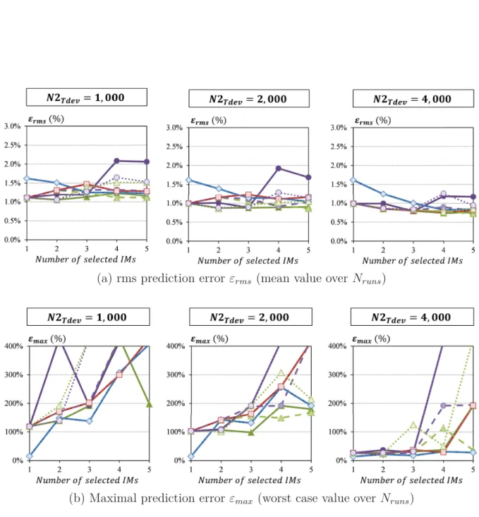
2.18 Prediction reliability for the transceiver test vehicle considering different IM selection strategies and different sizes of training set (mean value over Nruns) . 49 2.19 Comparative analysis of the different IM selection strategies for the two test vehicles . . . 50
3.1 Pareto scaling graph for the first ten principal components . . . 55
3.2 Correlation coefficient for MARS models built using an increasing number of IMs selected in the first PC . . . 56
3.3 Scatter graph for model built using the 30 highest-ranked IMs in the first PC . 56 3.4 Correlation coefficient computed on training set for models built on reduced IM space using PCA-based selection . . . 57
3.5 IM-space reduction based on MARS built-in selection feature . . . 58
3.6 Correlation coefficient for models built during iterative MARS-based selection 60 3.7 Correlation coefficient computed on training set for models built on reduced IM space using iterative MARS-based selection . . . 61
3.8 Extended SFS-Parental strategy . . . 62
3.9 Extended SFS-Parental strategy: IM combination lists . . . 63
3.10 Extended SFS-non Parental strategy . . . 64
3.11 Extended SFS-Non Parental strategy: IM combination lists . . . 64
3.12 Model accuracy for the transceiver test vehicle . . . 67
3.13 Model accuracy for the PA test vehicle . . . 67
3.14 Prediction accuracy for the transceiver test vehicle . . . 69
3.15 Prediction accuracy for the PA test vehicle . . . 70
3.16 Prediction reliability for the transceiver test vehicle . . . 73
3.17 Prediction reliability for the PA test vehicle . . . 73
3.18 Influence of IM space reduction options on prediction reliability for the transceiver test vehicle . . . 75
3.19 Influence of extended-SFS options on prediction reliability for the transceiver test vehicle . . . 77
3.20 Influence of extended-SFS options on prediction reliability for the PA test vehicle 77 4.1 Comparison between prediction reliability results evaluated on training and validation sets . . . 80
4.2 Two-tier alternate test synopsis with guard-band allocation . . . 81
4.3 Two-tier alternate test synopsis with model redundancy . . . 82
4.4 Procedure for confidence estimation based on model redundancy . . . 83
4.5 Overview of the proposed generic framework . . . 84
4.6 Meta-model construction with cross-validated committees (k=10) . . . 85
4.7 Exploration of cost-reliability tradeoff, for a given IM subset size . . . 86
4.8 Prediction reliability for models built with 3 IMs (models generated from extended-SFS) . . . 88
4.9 Accuracy and reliability metrics for redundant models vs. size of selected IM subsets . . . 89 4.10 Evaluation of different model redundancy implementations: (a) FPR vs.
di-vergence threshold, (b) Retest vs. didi-vergence threshold, (c) FPR vs. Retest . . 91 4.11 Prediction reliability achieved by different implementations of model
redun-dancy, for 3 values of acceptable Restest level . . . 92 4.12 Trade-off between test cost and test reliability for different sizes of selected
IM subsets (minimum front of FPR obtained from the different scenarios of redundant model generation) . . . 93
1.1 Test vehicle databases . . . 15
2.1 Number of outliers eliminated from the PA database for different values of k . 27 2.2 Number of outliers eliminated from the transceiver database for different values of k . . . 28
2.3 Test vehicle databases after outlier filtering . . . 30
2.4 Selected IM subsets for the PA test vehicle according to different selection strategies, different training set sizes, and different values for the maximum number of IMs used to predict the performance . . . 40
2.5 Selected IM subsets for the PA test vehicle according to different selection strategies, different training set sizes, and different values for the maximum number of IMs used to predict the performance . . . 42
2.6 Computational time for the transceiver test vehicle . . . 43
3.1 Evaluation of IM space reduction solutions . . . 61
3.2 Rms training error of generated models for the transceiver test vehicle . . . 66
3.3 Rms training error of generated models for the PA test vehicle . . . 68
3.4 Rms prediction error of generated models for the transceiver test vehicle . . . 69
3.5 Maximal prediction error of generated models for the transceiver test vehicle . 70 3.6 Rms prediction error of generated models for the PA test vehicle . . . 71
3.7 Maximal prediction error of generated models for the PA test vehicle . . . 71
3.8 Failing prediction rate of generated models for the transceiver test vehicle . . . 72
3.9 Failing prediction rate of generated models for the PA test vehicle . . . 72
T
he only viable solutions to test analog/RF integrated circuits are the specification-oriented ones. In other words, the test procedures have to estimate the device spec-ifications for the pass/fail decision during the production phase. For RF and high performance analog devices, these procedures require expensive Automatic Test Equipment (ATE) with high-speed and high-precision analog/RF test resources. In addition to the di-rect ATE cost, the specific test environment increases the overall test cost as additional test facilities, test equipment maintenance and test development engineering [1].Furthermore, because signal integrity is mandatory for RF measurement we have to consider RF probing issues, coaxial cable interfacing, matching functionality and board to device con-tact [2]. This context is particularly critical during the wafer test. In order to encounter these issues, manufacturers usually perform DC and low frequency measurements at the Wafer Test Level and focus on RF performances at the Package Test Level [1]. However, such kind of test increases also the test cost because the defective devices are identified in a backward level. In other words, the cost of packaging phase of the failed device is added to the overall test cost. Besides, the high cost of test is also due to the long time required to test analog/RF de-vice. Indeed, the measurement of only one specification might be long and a large number of performances have to be measured. This is particularly true for some complex RF devices addressing RF multi-modes, which usually lead to an excessive test time. Moreover, as the analog/RF test resources are limited on RF testers, the multi-site test solutions are usually impossible for analog/RF devices [3].
Finally, because technologies scaling are following Moore´s laws, the latest manufacturing technologies (i.e. System-On-a-Chip, System-In-Package, and Trough Silicon Via 3D Inte-grated Circuits) offer very high density. In this context, it becomes impossible to access all the inner component´s primary inputs and outputs in order to provide stimuli and monitor test responses.
Several cost-reduced RF IC testing strategies have been proposed in the literature to over-come the cost and inabilities of specification-based testing for analog and RF circuits. We can cite techniques based on analog Built-In-Self-Test (BIST) and Design for Testability (DFT) [4]. Other solutions rely on improving RF probing technologies and measurements accuracy [5]. In this context, the "alternate test" strategy (also called "indirect test") has appeared as a novel and promising strategy especially at Wafer Test Level [6] [7].
Alternate test offers several advantages compared to the conventional analog/RF test prac-tices. The general goal of the alternate test strategy is to establish the correlation between
two data spaces: the "low-cost measurement space" (Indirect Measurement IM) and the "ex-pensive specification space". Based on machine learning and data mining tools, indirect test principle assumes that we can use simple and low-cost analog/RF measurements to decide what is considered as pass/fail devices during the production phase. This approach has been applied to various types of analog and RF circuits.
The general purpose of this PhD report is to establish a framework for an efficient imple-mentation of alternate test for analog/RF circuits. The target is not only the accuracy of performance estimation, but above all to ensure a high level of confidence in the implemented test flow. The PhD report is divided into four chapters.
The first chapter is an overview of the alternate test. After summarizing the main existing data-mining tools and approaches, we remind the steps to implement the alternate test ap-proach referring to the data-mining process. Then, we present different metrics to be used for the evaluation of the alternate test efficiency. We also introduce a new metric called Failing Prediction Rate (FPR) which was developed to assess the built model reliabilities. Finally, we compare the performance of some learning algorithms on our datasets in order to choose the appropriate algorithm for our framework.
In the second chapter, we present a complete study in order to build a robust single model. We firstly introduce a basic filter to remove aberrant circuits. Then, we perform a comparative analysis of various IM selection strategies, which is an essential step for efficient implementa-tion of this technique. The objective behind is to perform a robust strategy to build the best single correlation model.
In the third chapter, we develop two strategies for multi-model generation. The proposed strategies are based on a reduction phase of the explored IM-space. Comparative analysis on the proposed strategies and the techniques of the IM space reduction are then given.
In the fourth chapter, we present a generic framework for efficient implementation of alternate test. The propose implementation uses model redundancy. This involves an exploration of the tradeoff between cost and robustness. Furthermore in order to increase confidence, we have investigated an original option which consists in building the meta-models using ensemble learning.
Finally, the main contributions of this thesis are summarized in the conclusion and perspec-tives for future work are presented.
Chapter
1
Alternate test and data mining
Contents
1.1 Some principles of data mining . . . . 4
1.1.1 KDD Process . . . 5
1.1.2 Machine-learning Algorithms . . . 6
1.2 Indirect test . . . . 9
1.2.1 Introduction . . . 9
1.2.2 Classification-oriented indirect test . . . 10
1.2.3 Prediction-oriented indirect test . . . 10
1.3 Prediction-oriented indirect test strategy . . . . 11
1.3.1 Training phase . . . 13
1.3.2 Validation phase . . . 13
1.3.3 Production testing phase . . . 13
1.3.4 Problematic . . . 14
1.4 Metrics for test efficiency evaluation . . . . 14
1.4.1 Accuracy metrics . . . 15
1.4.2 Prediction reliability: Failing Prediction Rate (FPR) . . . 16
1.5 Choice of the regression algorithm . . . . 18
1.6 Summary . . . . 22
T
he conventional practice for testing analog and RF circuits is specification-oriented, which relies on the comparison between the measured value and tolerance limits of the circuit performances. While this approach offers good test quality, it often in-volves extremely high testing costs. Indeed, the measurement of analog or RF performances requires dedicated test equipment which has to follow the continuous improvement in the performances of new ICs generation. It becomes difficult and very expensive to find the in-struments to measure accurately the specifications. In addition to the high cost of Automated1.1. Some principles of data mining
Test Equipment (ATE), the nature of each individually measured performance may imply a repeated test setup which further increases conventional test time. Moreover, as design trends tend to integrate complex and heterogeneous systems in one package, new technical difficul-ties are added to the heavy test costs. For instance, it becomes impossible to access all the inner components primary inputs and outputs in order to provide stimuli and catch test re-sponses. Finally, in the case of RF signals; a key challenge is to perform RF measurements at wafer level due to probing issues, and applying wafer-level specification-based testing at 100% is rather impossible. In this context, numerous research works can be found over the past twenty years on this topic. These usually try to overcome the cost and inabilities of specification-based testing for analog and RF circuits.
Towards RF test cost reduction, some research is designed to compact the number and types of specification tests that are operated within the production testing phase [8] [9]. Others have proposed a substitute solution namely "alternate test" (also called "indirect test") which has emerged as an attractive solution. The proposed solution relies on the power of machine learning and data mining tools to establish a simple and low-cost analog/RF specification test. The idea is to replace the conventional analog or RF performance measurements by some simple and low-cost measurements. The fundamental principle is actually based on exploiting the correlation between these two. This correlation is mapped through a nonlinear and complex function that can be determined by the mean of machine-learning algorithms. This correlation is then exploited during the mass production testing phase in order to deduce the circuit performances using only those low-cost indirect measurements. This approach has been applied to various types of analog circuits, including baseband analog [6] [7][10], RF [11][12][13][14], data converters [15][16], and PLLs [17].
This indirect test approach requires data mining tools and additional treatments integrated on a complete test board process in order to find the best ways for its implementation. This chapter is organized as follows. Section 1.1 presents some principles of data mining. Section 1.2 presents the indirect test. Section 1.3 describes the prediction-oriented indirect test strategy. In section 1.4, we define the metrics that we will use with this work. Section 1.5 exposes a comparative study between 3 widely used regression algorithms in order to choose the appropriate machine-learning algorithm for our study. Finally, section 1.6 concludes the chapter.
1.1
Some principles of data mining
Data mining is the field that studies large data sets. The aim is to find models that can summarize big data in order to convert them later into information and then into knowledge [18]. More precisely, data mining algorithms aim to identify what is deemed knowledge according to the disposed features and try to extract the relevant patterns from data. Data mining is generally performed inside a multi-step process and it relies heavily on Machine Learning Algorithms (MLA).
1.1.1
KDD Process
The term Knowledge Discovery in Databases (KDD) refers to the board process of finding knowledge in data with the application of particular data mining methods. It is of interest to researchers in machine learning, pattern recognition, databases, statistics, artificial intel-ligence, knowledge acquisition for expert systems, and data visualization [19]. The unifying goal of the KDD process is to extract knowledge from data in the context of large databases. It involves the evaluation and possibly interpretation of the patterns to make the decision as to what qualifies as knowledge. It is a multi-step process that includes the choice of prepro-cessing, sampling, projections and data mining tools.
Figure 1.1: KDD
The KDD process involves the following steps:
⋄ Selection: creating a target data set on which discovery will be performed after understand-ing of the application domain.
⋄ Data cleaning and preprocessing: removal of noise or outliers, strategies for handling miss-ing data fields, feature scalmiss-ing...
⋄ Data reduction and projection: using dimensionality reduction or transformation methods to reduce the dataset while keeping useful features to represent the data depending on the goal of the task.
⋄ Data mining: deciding whether the goal of the KDD process is classification, regression, clustering, etc. Searching for the appropriate machine-learning algorithms and patterns of interest.
⋄ Analyze discovered knowledge: interpreting mined patterns
The KDD process coheres with the alternate test context. It corresponds actually to the classical implementation of an indirect testing flow. In this manuscript, we will perform the
1.1. Some principles of data mining
various described steps above with some adaptation to the alternate test context. Also, we will expose additional processing to achieve our objectives. More details on the indirect test-ing implementation will be found in the next sections.
1.1.2
Machine-learning Algorithms
Overview of Machine-Learning Algorithms
Machine-learning algorithms are one of the most exciting recent technologies. They are om-nipresent in our daily live and we are using them unconsciously. Website engines like Google use MLA to search in internet. Facebook or Instagram applications use MLA to recognize our friend photos. Spam filters save us from thousands of spam emails using MLA. Machine learning then tries to mimic how human brain learns and investigated in different complex fields.
MLA was developed as a new capability for computers and today it touches many statements of industry and basic science [20][21]. Data mining is one of the fields based on MLA. For example, biologists are performing MLAs on data collected from genes and ADN sequences to understand the human geneses [22]. All fields of engineering as well are using MLAs, engineers have big datasets to understand using learning algorithms. Also, MLAs are used to perform applications that can´t be programmed by hand as autonomies helicopter,where a computer learns by itself how to fly a helicopter based on MLAs [23].
Two kind of machine-learning algorithms exist: supervised and unsupervised machine-learning algorithms.
Figure 1.2 represents the two main families of MLA. For both graphs, X1 and X2 represent the features (also called attributes). We have considered in this example two features but obviously we can have more then 2. The two MLA families are:
⋄ Supervised learning: is a learning problem where, for a given dataset, the features are labeled and the output space(class)is known. Two kinds of problems can be solved with supervised learning algorithms:
Regression problem: is one of the most popular statistical problems among the data mining community. Regression algorithms try to look for a law which connects something that is continuous in input with something that is continuous in output. As a regression problem example, housing price prediction where we want to predict the price of houses according to the house sizes.
Classification problem: consists in associating an individual X to a class C from K classes based on their types, properties and behaviors. The input space is divided in two or more classes. Example, classify patient as holder of a malignant tumor (class 1) or benign tumor (class 0) regarding the tumor size.
⋄ Unsupervised learning: in this case, for a given data set, we don´t know either data labels or to which group the data belongs and we want to find some structure in the data for clustering issues. This can make it hard to reveal the information contained in those data
sets. This problem is considered to be as an unsupervised problem and should be solved by an approach called Clustering [24]. As example, Google news use clustering algorithms every time we are searching for news on the Internet. It displays thousands of different pages related to the same news topic that we are searching for and where it clusters auto-matically the same topics.
(a)Regression (b)Classification (A) Supervised learning algorithms
(B)Unsupervised learning algorithms
Figure 1.2: Machine-learning algorithms
In our study, we are in the supervised learning context as both input and output variables are defined. The next section focuses on two kinds of potential algorithms: regression and classification algorithms.
Regression Algorithms
There are several machine-learning algorithms used for regression mapping. In the same way, in the field of indirect testing, people used various algorithms [25]. We define below briefly three of the most commonly used learning algorithms:
⋄ Artificial Neural Network (ANN) is a mathematical model inspired from biological neural networks, which involves a network of simple processing elements (neurons). ANN is a
1.1. Some principles of data mining
multi-layered system composed of an input, hidden and output layers. Through the mul-tiple layers of the network, a back propagation algorithm is used to adjust the parameters and threshold value of the network in order to minimize the error value for all inputs. Neural networks can be used for modeling complex relationships between inputs and out-puts and they have been successfully implemented for prediction tasks related to statistical processes. Although ANN is very useful, it has some drawbacks. It is computationally expensive. Also, it is a black box learning approach: we cannot interpret relationships between inputs, layers and outputs. The difficulty in using ANN comes with the choice of the number of neurons. On the one hand, too few neurons lead to high training and generalization errors due to underfiting and high statistical bias. On the other hand, too many neurons lead to low training errors but high generalization error due to overfiting and high variance.
⋄ Regression trees can be defined as a set of rules. It starts with all the data in one node and then splits it into two daughter nodes depending on the implemented rules. Each daughter node is then split again. This process is repeated on each derived daughter in a recursive manner. The recursion is completed when the subset at a node has all the same values of the target variable, or when splitting no longer adds value to the predictions [26]. One of the questions that arises in a regression trees algorithm is the optimal size of the final tree. A tree that is too large risks overfitting the training data and poorly generalizing to new samples. A small tree might not capture important structural information about the sample space.
⋄ Multivariate Adaptive Regression Splines (MARS) is a series of local regressions stitched together to form a single function presented for the first time by J. Friedman in [27]. It can be considered as an adaptation of the regression tree. It is a multiply looped algorithm that has a spline function in the innermost loop.
The MARS model can be viewed in the following form:
â f (x) = c0+ k Ø k=1 ciBi(x) + k Ø k=2 ci,jBi,j(xi, xj) + k Ø k=3 ci,j,kBi,j,k(xi, xj, xk) + ... (1.1)
where B corresponds to the basis function, c is the weighting coefficient, and c0 is the
con-stant intercept term. The model is a sum of a sum of all basis functions that involve one variable, two variables, three variables and so on. During the construction of the predictive model, there is a first forward phase in which a greedy algorithm is used to select basis functions, i.e. the algorithm iteratively adds reflected pairs of basis functions. For each pair of basis functions added, a model is built and its performance evaluated in terms of training error. At each iteration, the algorithm selects the pair of basis functions that gives the largest reduction of training error. There is then a backward phase in which the algo-rithm removes terms one by one, deleting the least effective term at each step (according to the GVC criterion), until a user-configurable limit of maximum allowed basis functions is reached (NBFmax). MARS models are most useful in high dimensional spaces where there is little substantive reason to assume linearity or a low level polynomial fit. They combine very flexible fitting of the relationship between independent and dependent variables with model selection methods that can sharply reduce the dimension of the model [28]. MARS is quite recommended for continuous data processing. We will base our study on this
al-gorithm. Reasons and detailed explanation will be found in the last section and the next chapter.
Classification Algorithms
Several classification algorithms exist to deal with classification problems. There are some algorithms that are assigned for classification problems as the K-NN, ZeroR, OneR...
Furthermore, other algorithms such as ANN and Support vector machine (SVM) can be used for classification issues.
⋄ K-Nearest Neighbors (K-NN): the principle is to classify a new sample on its appropriate class. According to the chosen K value, the algorithm computes the distance between the K nearest neighbors (nearest individuals) and the new sample. The number of the nearest neighbors determines the class to where the new individual belongs. KNNs are fast and simple to implement. The big issue related to the use of K-NN is to find the optimal con-figuration (the appropriate number of classes).
⋄ Support vector machine (SVM): is a supervised learning algorithm which can be used for classification or regression. SVM constructs separating hyperplane for the classes, and tries to find the hyperplane with the maximum margin between the classes. Samples on the margin are called the support vectors [29].
As some MLA matters with feature scaling (MLA that depends on distances and uses gradi-ent descgradi-ent)[30], generally data analysts perform during the data preprocessing step a data normalization. We have used the rescaling and standardization techniques for the "low-cost indirect measurements" and performances respectively. The corresponding formulas for the rescaling and standardization techniques are respectively:
x′ = x − min(x)
max(x) − min(x) (1.2)
x′ = x − ¯x
σ(x) (1.3)
where x is the original feature vector, x’ is the normalized value, ¯x is the mean of that feature vector, and σ is its standard deviation. Feature rescaling resizes the range of features to scale the range in [0, 1] or [−1, 1]. Feature standardization makes the values of each feature have zero-mean (when subtracting the mean in the enumerator) and unit-variance. Both methods are widely used for normalization in many machine learning algorithms (e.g., support vector machines, logistic regression, and neural networks).
1.2
Indirect test
1.2.1
Introduction
The underlying idea of alternate testing is that process variations that affect the conventional performance parameters of the device (individual) also affect non-conventional low-cost
indi-1.2. Indirect test
rect parameters. If the correlation between the indirect parameter space (attributes) and the performance parameter space (classes) can be established, then specifications may be verified using only the low-cost indirect signatures. However the relation between these two sets of parameters is complex and usually cannot be simply identified with an analytic function. Two main directions have been explored for the implementation of the indirect test; the classifica-tion and the predicclassifica-tion-oriented strategies.
Below, for the given 2D illustrations, we present the Indirect Measurement Space by IM = [IM1, IM2, ..., IMm] , the Circuit Performance Space by P = [P1, P2, ..., Pl] and the
Specifi-cation Tolerance Limits by Limits = [Pp, min, Pp, max] .
1.2.2
Classification-oriented indirect test
The "classification-oriented strategy" was examined in many studies in the literature [9] [31] [32] [33] [34]. The principle is to classify devices as good or faulty (PASS/FAIL) without pre-dicting its individual performance parameters. In such kind of study we evoke a classification problem where the specification tolerance limits are therefore part of the strategy. As figure 1.3 illustrates, the PASS/FAIL decision is fixed on the IM space. The specification tolerance limits are used only on the learning step in order to build the decision boundaries on the IM space. After that, the performance space is no more used and only the learned boundaries will serve to classify any new device into the class it belongs to.
On one hand, this strategy seems to be as fast as the PASS/FAIL decision is made on the IM space without turning back to the specification space and without verifying the RF per-formances of the new devices. On the other hand, this approach cannot offer diagnosis capability. The other drawback is the necessity to have the specification tolerance limits from an early phase (learning phase). Indeed, in mass production testing the specification limits may change.
Figure 1.3: Classification-oriented testing
1.2.3
Prediction-oriented indirect test
The second strategy, the "prediction-oriented strategy", was adopted in many studies [7] [35] [36]. This strategy evokes a prediction problem where an estimation of the measured performances is provided by the end. Figure 1.4 illustrates the principle.
Figure 1.4: Prediction-oriented testing
The device performances are predicted instead of the decision boundaries by the regression model. On the prediction-oriented testing, the specification tolerance limits are known only on the production test phase unlike its counterpart "classification-oriented testing". The PASS/FAIL decision is made once the specification tolerance limits are provided.
This strategy has several advantages compared to the classification-oriented strategy. The main advantage is the potential use of the predicted specifications to adjust test production limits. Moreover, information about the predicted performances helps to diagnose, interpret and build confidence on the indirect test flow.
We have adopted the prediction-oriented strategy in our work due to these advantages. More details on the prediction-oriented testing will be found in the next section.
1.3
Prediction-oriented indirect test strategy
Figure 1.5 summarizes the prediction-oriented indirect testing synopsis, which involves three distinct phases: training, validation and mass production testing phases. Let P = P1, P2, ..., Pl
denote the l performances of the Device Under Test (DUT) that need to be evaluated with the conventional specification prediction-oriented test approach, and IM = [IM1, IM2, ..., IMm]
a pattern of m low-cost indirect measurements. Note that the alternate test relies on the as-sumption that the DUT is affected by process variations but does not contain a hard defect. A defect filter such as the one proposed in [32] should therefore be included in the production testing phase in order to screen out circuits affected by hard defect before they are sent to the regression models.
One of the crucial issues associated with the indirect test approach consists in developing a model that satisfies the following challenges:
⋄ High model accuracy: the regression model has to accurately represent the relationship between selected indirect parameters and specifications to be predicted.
⋄ High prediction reliability: specifications have to be correctly predicted for all devices evaluated during the production test phase, although the model is built on a limited number of training instances.
⋄ Low-cost model: the built model has to discount the test cost. The indirect test technique has to involve the minimal number of IMs as possible to ensure a low-cost test implemen-tation.
1.3. Prediction-oriented indirect test strategy
1.3.1
Training phase
During this phase, a set of devices so-called "Training Set" (TS) is assigned to feed a learning algorithm in order to build a regression model. The learning algorithm has two kinds of information as input: the low-cost indirect measurement dataset (IMs) and the conventional performance measurement (P) that were extracted from the TS. A regression model dedicated to the targeted performance is obtained as output. That means that for each performance parameter Pj, a machine-learning algorithm is trained over the two sets of measurements to
build the regression model fj : [IM1, ..., IMm] → Pj.
At this level, the model has to ensure a high accuracy; it has to accurately represent the relationship between selected indirect parameters and specifications to be predicted. The evaluation of the model accuracy is established by some specific metrics that we will intro-duce later on. Different regression tools can be employed, including polynomial regression, Multivariate Adaptive Regression Splines (MARS), Artificial Neural Networks (ANNs), sup-port vector machines (SVMs), etc. Obviously, the quality of a regression model is strongly related to the choice of the input information (IMs) used to build the regression model. These indirect measurements have to be information-rich and correlate well with the device perfor-mances. Also, the appropriate choice of the learning algorithm to use will boost for sure the performance of the built model. Furthermore, the training devices and the training set size to consider theoretically have an impact on the built model. All these parameters have to be well fixed at this first phase of the indirect test synopsis. It is therefore also the objective of our work to analyze this aspect and more details will be given later on in the manuscript.
1.3.2
Validation phase
Following the training phase, a validation phase is executed. This phase is required to assess the built model efficiency. This evaluation is made on another set of devices so-called "Vali-dation Set" (VS). The vali"Vali-dation set disposes of the same kind of information as the training set but extracted from a different set of devices (VS).
Some classical metrics have been widely used in the literature to evaluate the prediction accu-racy on VS. We will expose them and discuss their efficiency in the next paragraph. Moreover, we will introduce a new metric to assess the prediction reliability.
To achieve a viable efficiency assessment, the training and validation sets must have similar statistical properties. In this respect, we have used the LHCS "Latin Hyper-cube Sampling" process to divide the experimental dataset into two twin sets [37]. When the built regression model is evaluated in terms of prediction accuracy and reliability, we will be able to launch the production testing phase.
1.3.3
Production testing phase
In the production phase concerning a huge number of devices, we measure only one kind of information: the low-cost indirect measurements for each production device. The built regression model is then used to predict the corresponding RF performances based only on that information. After predicting the new device performances, we resort to the specification tolerance limits in order to classify the devices on PASS and FAIL classes.
1.4. Metrics for test efficiency evaluation
1.3.4
Problematic
By adopting the prediction-oriented testing, crucial challenges have to be faced in order to es-tablish a confident and efficient alternate test implementation. In fact, during the production testing phase, the high-priced performances are predicted by the mean of the "low-cost mea-surements" for a huge number of instances. Those predicted RF values suffer from a lack of confidence from industrials. The lack of confidence comes from different points. Dependency of prediction model with the training phase settings (the used IMs and TS) affects the model robustness and then the confidence in the strategy efficiency. Also, as the model is built on a limited number of training instances, an expression of a durable robustness is difficult face the set of production devices. Another point, many studies have shown that large prediction errors can be observed once implementing the prediction-oriented testing, which is not toler-ated from industrials.
Those challenges can be exposed in the form of the following questions: How to improve confidence in indirect test?
How to build an accurate and robust model?
Should we rely on a single model to predict all devices? How to select pertinent IM subset(s)?
How to safely clean-up dataset(s)?
Which learning devices and which training set size should we consider? How to make an efficient test and which test metrics to use?
How to manage the trade-offs between test cost and test reliability?
How to implement a generic and robust indirect test flow suitable for a given application? Actually some of those problems have already been the focus of previous studies. We will try to answer all these questions in this manuscript along with proposing our contributions. Due to the limited time, other points were not included in the objectives of this work. They will be presented as further perspectives.
Two test vehicles fabricated by NXP Semiconductors will be used in this thesis to support the investigations and evaluate our propositions. The first one is a Power Amplifier (PA) for which we have production test data on a large set of devices, i.e. more than 10,000 devices. These data include 37 low-cost indirect measurements and one conventional RF performance measurement. The second test vehicle is a more complex device, i.e. an RF transceiver, for which we have experimental test data from a more limited set of devices, i.e. around 1,300 devices. These data include one conventional RF performance measurement and a large number of indirect measurements, i.e. 405 indirect measurements. Table 1.1 summarizes the composition of the databases provided by NXP, for the two test vehicles.
1.4
Metrics for test efficiency evaluation
A key issue for the deployment of the indirect test strategy is test efficiency evaluation. This latter is usually evaluated in terms of prediction accuracy and the most classical metric used in the literature is the average or rms error; maximal error is also sometimes reported.
How-Table 1.1: Test vehicle databases
Test vehicle Number of circuits Number of IMs Number of measured Performances (Ps)
PA 11207 37 1
Transceiver 1299 405 1
ever these metrics do not give any information on prediction reliability, i.e. how many of the circuits are evaluated during the mass production test with a satisfying accuracy.
In this section, we first define the classical accuracy metrics and then, we introduce a new metric related to prediction reliability. These metrics will be used all along this manuscript for test efficiency evaluation.
1.4.1
Accuracy metrics
In this work, we will use as accuracy metrics the rms error (computed as the Normalized Root Mean Square Error N RM SE) and the maximal error, which are defined by:
εrms= 1 Pj | nom ö õ õ ô 1 Ndev Ndev Ø i=1 (P(j, i) − ˆP(j, i))2 (1.4) εmax = max(| P(j, i) − ˆP(j, i) |) Pj | nom (1.5) where Ndev is the number of evaluated devices, P(j, i) is the actual performance value of the
ith device, and ˆP
(j,i) is the predicted jth performance value of the ith device. These metrics
are expressed in percentages through normalization with the jth nominal performance value
Pj | nom. The lower these metrics, the better the accuracy is.
Note that we can distinguish model accuracy and prediction accuracy depending on whether metrics are computed on the Training Set (TS) or on the Validation Set (VS)[38].
Model accuracy
Model accuracy is usually evaluated by computing εrms on training devices. In this case, the
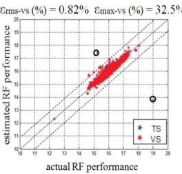
metric reveals the intrinsic model accuracy, i.e. the global ability of the model to accurately represent the correlation between the used indirect measurements and the device performance under consideration. Figure 1.6 shows a scatter plot example of estimated versus actual per-formance on the training set. This kind of graph gives a qualitative estimation of the model accuracy: a model is considered accurate when the learning devices (plotted with blue dots) follow the first bisector. The rms error gives a quantitative evaluation of how close the blue dots are to the first bisector.
1.4. Metrics for test efficiency evaluation
Figure 1.6: Example of estimated vs. actual RF performance on the TS
Prediction accuracy
Prediction accuracy is usually evaluated by computing εrms on devices of the validation set.
In this case, the metric actually reveals the global ability of the model to accurately predict performance values for new devices. Figure 1.7 shows a scatter graph example of estimated versus actual performance on the training and validation sets (TS and VS). It can be observed that the large majority of validation devices (plotted with red dots) are accurately predicted, resulting in a low rms prediction error (in the same range as the rms error evaluated on TS). However it can also be observed that some devices exhibit a high prediction error. This is not expressed by the rms error since the number of these devices is extremely small compared to the number of devices correctly predicted; in contrast this is clearly expressed by the maximal prediction error. The maximal prediction error, which is not always reported in the literature, permits us to pinpoint this situation.
In our work, we evaluate both rms and maximal prediction errors.
1.4.2
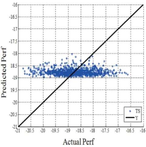
Prediction reliability: Failing Prediction Rate (FPR)
The rms and maximal prediction errors allow us to quantify prediction accuracy but they are not sufficient to evaluate indirect test efficiency. Actually, many experiments reported in the literature on various devices demonstrate that very low average prediction errors can be achieved but this does not guarantee low maximal prediction error. This problem was highlighted in several studies [38] and [39]. Also, as evaluation is usually performed on a small set of validation devices (hundreds to some thousand instances) even if low maximal prediction error can be observed on a small validation set, there is no guarantee that the maximal prediction error will remain in the same order of magnitude when considering the large set of devices under test (several millions of devices). Finally it should be highlighted that the maximum prediction error is only an indicator of the worst case error, but gives no indication of the number of devices affected by a large prediction error.
Figure 1.7: Example of estimated vs. actual RF performance on the VS
In this context we define a new metric dedicated to prediction reliability, which is related to the number of devices that are predicted with a satisfying accuracy for a given set of de-vices. More precisely this metric, called Failing Prediction Rate (FPR) [40], is defined as the ratio between the number of devices with a prediction error higher than a given εmeas and
the number of devices in the validation set, where εmeas corresponds to the measurement
re-peatability error achieved when performing conventional measurement of the targeted circuit performance Pj.
The FPR, expressed in percentage, is given by: F P R(εmeas) = 1 NV dev NØV dev i=1 (| P(j, i) − ˆP(j, i) |> εmeas) (1.6) where: |P(j, i) − ˆP(j, i)| > εmeas= I 1 if true, 0 otherwise.
This metric permits us to quantify the indirect test efficiency with respect to the conventional test since it represents, for each circuit performance Pj to be evaluated, the percentage of
circuits with a prediction error that exceeds the conventional measurement uncertainty. It is therefore a relevant metric to evaluate prediction reliability; it can also be used to compare the different Indirect Measurement (IM) selection strategies that we will introduce in the next chapter. As an illustration, figure 1.8 gives the FPR computed on the validation set for two models built with different combinations of indirect measurements. We can notice from this figure that the percentage of devices with a prediction error higher or equal to the conventional measurement uncertainty εmeasresulting from Model 2 is less than the one given
by Model 1; we can thus conclude that Model 2 offers better prediction reliability than Model 1.
1.5. Choice of the regression algorithm
Figure 1.8: An example of Failing Prediction Rate (FPR) achieved with two different models
1.5
Choice of the regression algorithm
Various regression algorithms can be employed to build the regression model, including poly-nomial regression, Multivariate Adaptive Regression Splines (MARS), Artificial Neural Net-works (ANNs), Support Vector Machines (SVMs), etc. To motivate the choice of the appro-priate machine-learning algorithm for our indirect testing flow, we have made a preliminary comparative study between 3 three widely used regression tools: the MARS, the ANN and the Regression Tree algorithms (implemented in ENTOOL Matlab-toolbox for regression mod-eling [41]). We can find brief first comparison studies on one of these algorithms efficiency in [42], but only in terms of accuracy (evaluated through Mean Square Error, MSE) on one case study. We extend here this study by comparing the performance achieved by the three algorithms not only in terms of accuracy but also in terms of reliability by exploiting the new FPR metric.
Practically for each test vehicle, we have selected a subset of 3 pertinent indirect measure-ments. These indirect measurements were provided to the different algorithms and a regression model was built for each MLA; Our analysis is based on two practical case studies: a Power Amplifier (PA) and an RF transceiver from NXP semiconductors. The assessment relies on the training and validation errors that were then computed on both test vehicles. Note that to ensure a meaningful comparison, we have used the same training and validation sets that were used for the 3 studied MLAs. Results are summarized in figures 1.9 and 1.10 for the PA and transceiver test vehicles respectively. Intrinsic Model model accuracy is evaluated by the rms error computed on the training set (εrms−T S), while prediction accuracy is
eval-uated by the rms and maximal prediction errors computed on the validation set (εrms−V S) and εmax−V S), and prediction reliability is assessed by the new failing prediction rate metric (FPR). Different remarks derive from those graphs.
(a) Classical metrics
(b) FPR metric
1.5. Choice of the regression algorithm
(a) Classical metrics
(b) FPR metric
First regarding the classical metrics:
- the different MLAs lead to similar performance in terms of intrinsic model accuracy with
equivalent rms errors on the TS;
- a modest advantage can be observed for the MARS algorithm in terms of prediction
ac-curacy since it permits us to preserve the same rms error on the VS and exhibits the lowest maximal error. These results are in accordance with the previous study reported in [42].
Then regarding prediction reliability evaluated by the new metric, we can notice a clear advantage of the MARS algorithm over the two other algorithms, since it permits us to achieve the lowest FPR for both test vehicles. Based on these observations, we could conclude that the MARS algorithm leads to more reliable models than the ANN and the Regression Tree algorithms. From this study, we have decided to use the MARS algorithm to build regression models for the rest of our work.
1.6. Summary
1.6
Summary
Reducing the analog/RF IC test cost is a crucial issue in the semiconductors industry. There is a significant need to develop alternate techniques to the classical test approaches. Indirect test technique was proposed in order to lower the test cost. This approach is well known in the field of analog/RF IC testing but it suffers from a lack of confidence from industrials. Different steps to implement a robust indirect test flow are required. For this purpose, indi-rect testing as many research fields relies on the data mining tools and takes into account the KDD process in order to ensure the best exploration of the data space.
In the first part of this chapter, we have swiftly cited the different steps to implement the indirect test approach. We have mentioned some difficulties related to the application of the KDD process in our context. In fact, the effectiveness of a model is affected by several pa-rameters. The case study and problem type are the key to identify the best data mining and MLA tools to use. Also, the data preprocessing step (as data cleaning and feature scaling) affect the prediction qualities. Another basic parameter is the right choice of training and validation sets. Those sets have to be split in a proper manner to equally present knowledge in data. Furthermore, other parameters can badly affect the model accuracy such as underfitting and overfitting problems. For this purpose data scientists refer to some estimation procedure (as cross-validation) in the case of very limited data sets or combine models to enhance the predictions qualities.
In the second part, we have announced our choice to work with the prediction-oriented in-direct test strategy and we have exposed the different challenges that we have to deal with among this study. Also we have presented the different metrics used to evaluate the indi-rect test efficiency. Besides, we have introduced a new metric called FPR to assess the built model reliabilities. Finally, we have compared the performance of 3 commonly-used Machine-Learning Algorithms on our datasets and we have chosen to exploit the MARS algorithm for the implementation of the indirect test strategy.
In the next chapter we will come back to the different steps to build the prediction-oriented indirect test strategy. We will explain: the different steps, the different comparison analysis made and the additional processing to be integrated within the classical indirect test flow in order to develop a robust and generic indirect test implementation.
Chapter
2
Single model approach: outlier filtering and
selection of indirect measurements
Contents
2.1 Outlier filtering . . . . 25 2.1.1 Exploratory IC space analysis . . . 26 2.1.2 Adaptive k-filter . . . 26 2.2 Methods for indirect measurement selection . . . . 30 2.2.1 IM selection based on Pearson correlation . . . 32 2.2.2 IM selection based on Brownian distance correlation . . . 33 2.2.3 IM selection based on SFS algorithm . . . 34 2.2.4 IM selection using MARS built-in selection feature . . . 36 2.3 Experimental setup for the evaluation of IM selection methods 36 2.3.1 IMs selection . . . 37 2.3.2 Indirect test efficiency evaluation . . . 38 2.4 Results and discussion . . . . 39 2.4.1 IM selection . . . 39 2.4.2 Test efficiency . . . 43 2.5 Summary . . . . 51
B
igdata is used to describe a massive volume of data. It is used in many fields: finance, marketing, biology, tourism... When dealing with such large amounts of data we face difficulties in being able to manipulate, and manage them. Computation time, storage difficulties volume, visualization and plotting big data represent serious issues for big data. In the context of indirect testing, the database contains a set of measurements, composed of m indirect measurements (IMi, i = 1, ..., m) and p performance measurements (Pj, j = 1, ..., p),extracted from a population of n integrated circuits (ICk, k = 1, ...n). The typical structure
ICk) while the columns represent the attributes (indirect measurements, IMi) and the classes
(performance measurements, Pj) associated with the individuals. The objective is to explore
the possible correlation between the attributes and the classes in order to establish a regression model for each class. These models will then be used to predict performance values of new individuals.
Figure 2.1: Database form representation as a table of individuals (ICk), attributes (IMi) and
classes (Pj)
The regression model ensuring the correlation between the attributes and a given class is then the cornerstone for accurate prediction. Two main issues have to be faced for the construction of efficient regression models:
⋄ The presence of outliers in the database: An outlier can be defined as "an observation that deviates so much from other observations as to arouse suspicion that it was generated by a different mechanism" [43]. In the context of regression analysis, the problem with the presence of outliers in the database is that, since they are not consistent with the statistical nature of the remainder of data, they can affect the quality of the regression model. Therefore, they should be excluded from the database prior to the construction of the regression models.
⋄ The curse of dimensionality: The curse of dimensionality refers to various phenomena that arise when analyzing and organizing data in high-dimensional spaces. In the context of regression analysis, it may seem interesting to have as many attributes as possible to maximize the opportunity to build a satisfactory model. However taking into account more attributes does not necessarily lead to a better model. In fact with a fixed number of training samples, the predictive power of a regression model reduces as the dimensionality increases, and this is known as the Hughes effect or Hughes phenomenon [44]. To avoid such an issue, regression models should involve an only limited number of attributes; selection methods are therefore required to identify the most pertinent attributes.
In this chapter, we address these two aspects. First we present an adaptive k-filter that permits us to remove outliers from the database. Then we investigate feature selection algorithms and more precisely we explore four different strategies for the selection of indirect measurements in order to avoid the curse of dimensionality issue. An experimental setup is developed to perform a comparative analysis of these strategies and results are evaluated on the two test vehicles for which we have production test data.
2.1
Outlier filtering
Alternate testing relies on the construction of a regression model that maps one device perfor-mance to some indirect measurements. It is well-established that such a regression function can be fit for data that are described by a fixed probability density function [45]. Outliers should therefore be excluded from the training phase since they are not consistent with the statistical characteristics of the remainder of the data.
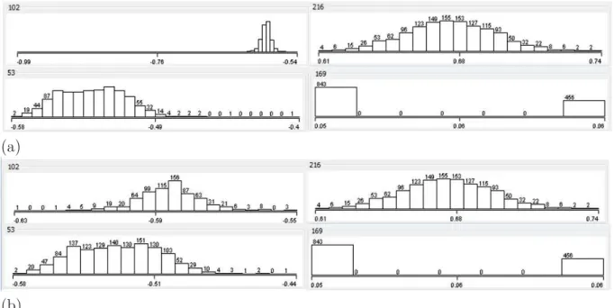
In this work, we admit that outlier circuits are those whose measurement appears to deviate markedly from other circuits of the database. Generally outlier circuits correspond to circuits affected by random manufacturing defects, leading their measurement value to lie outside of the measurement statistical distribution. As an illustration, figure 2.2 shows the histogram distribution of an indirect measurement for the transceiver test vehicle. The indirect mea-surement of some circuits is so far from the mean of the IM distribution that they can be considered as outliers; those circuits should be identified and eliminated from the training dataset since they may adversely affect the quality of the learned regression model.
Figure 2.2: Histogram distribution for an indirect measurement over the IC population showing outlier circuits
Outlier detection has been studied for decades in a number of application domains such as fraud detection, activity monitoring, satellite image analysis or pharmaceutical research, but there is no single universally applicable technique [46]. In the context of alternate testing, a defect filter based on joint probability density estimation has been developed [32] to identify outliers that do not fit the expected multi-dimensional distribution of the indirect measure-ments. However this defect filter suffers from computational issue in the case of indirect measurement space with high-dimensionality. Another method consists in allocating non-linear guard-bands in the indirect measurement space [47]; however correct positioning of the guard-bands requires information on defective devices which is not always available. In this section, we develop a simple filter, so-called "adaptive k-filter" that can handle IM space of high-dimensionality and does not require information on defective devices. An exploratory analysis of the IC space is first presented in sub-section 2.1.1 for a better understanding of our database elements and a better setting of the filter requirements. The filter proposed for