Past Market Variance and Asset Prices

Texte intégral

(1)2011s-16. Past Market Variance and Asset Prices Federico M. Bandi, Benoit Perron. Série Scientifique Scientific Series. Montréal Cette version mars 2010 This version March 2010 (CIRANO publication : février 2011/February 2011). © 2011 Federico M. Bandi, Benoit Perron. Tous droits réservés. All rights reserved. Reproduction partielle permise avec citation du document source, incluant la notice ©. Short sections may be quoted without explicit permission, if full credit, including © notice, is given to the source..

(2) CIRANO Le CIRANO est un organisme sans but lucratif constitué en vertu de la Loi des compagnies du Québec. Le financement de son infrastructure et de ses activités de recherche provient des cotisations de ses organisations-membres, d’une subvention d’infrastructure du Ministère du Développement économique et régional et de la Recherche, de même que des subventions et mandats obtenus par ses équipes de recherche. CIRANO is a private non-profit organization incorporated under the Québec Companies Act. Its infrastructure and research activities are funded through fees paid by member organizations, an infrastructure grant from the Ministère du Développement économique et régional et de la Recherche, and grants and research mandates obtained by its research teams. Les partenaires du CIRANO Partenaire majeur Ministère du Développement économique, de l’Innovation et de l’Exportation Partenaires corporatifs Banque de développement du Canada Banque du Canada Banque Laurentienne du Canada Banque Nationale du Canada Banque Royale du Canada Banque Scotia Bell Canada BMO Groupe financier Caisse de dépôt et placement du Québec Fédération des caisses Desjardins du Québec Financière Sun Life, Québec Gaz Métro Hydro-Québec Industrie Canada Investissements PSP Ministère des Finances du Québec Power Corporation du Canada Raymond Chabot Grant Thornton Rio Tinto State Street Global Advisors Transat A.T. Ville de Montréal Partenaires universitaires École Polytechnique de Montréal HEC Montréal McGill University Université Concordia Université de Montréal Université de Sherbrooke Université du Québec Université du Québec à Montréal Université Laval Le CIRANO collabore avec de nombreux centres et chaires de recherche universitaires dont on peut consulter la liste sur son site web. Les cahiers de la série scientifique (CS) visent à rendre accessibles des résultats de recherche effectuée au CIRANO afin de susciter échanges et commentaires. Ces cahiers sont écrits dans le style des publications scientifiques. Les idées et les opinions émises sont sous l’unique responsabilité des auteurs et ne représentent pas nécessairement les positions du CIRANO ou de ses partenaires. This paper presents research carried out at CIRANO and aims at encouraging discussion and comment. The observations and viewpoints expressed are the sole responsibility of the authors. They do not necessarily represent positions of CIRANO or its partners.. ISSN 1198-8177. Partenaire financier.

(3) Past Market Variance and Asset Prices. *. Federico M. Bandi †, Benoit Perron ‡. Abstract Recent work in asset pricing has focused on market-wide variance as a systematic factor and on firm-specific variance as idiosyncratic risk. We study an alternative channel through which the variability of financial market returns may help our understanding of cross-sectional price formation in financial markets. Invoking the countercyclical nature of market variance, we allow the (stochastic) discounting of future cash-flows to depend on the level of past market variance (pmv). Employing pmv as a conditioning variable in a classical consumption-CAPM framework, we derive economically meaningful conditional factor loadings and conditional risk premia. We show that scaling by pmv may also yield more effective pricing results than scaling by successful, alternative variables (such as the consumption-to-wealth ratio) precisely at frequencies at which their predictive ability for excess market returns should be (in theory) and is (empirically) maximal, i.e., business-cycle frequencies. Keywords: Asset prices, financial markets.. *. We thank Eric Jacquier, Pietro Veronesi, and participants in the Financial Econometrics Conference at Imperial College, London (May, 2008), and the Inaugural Meetings of the Society for Financial Econometrics (SoFiE) for helpful comments. Financial support from the William S. Fishman Faculty Research Fund at the Graduate School of Business of the University of Chicago (Bandi) and FQRSC, SSHRC, and MITACS (Perron) is gratefully acknowledged. Both authors also thank the Initiative on Global Markets at the Booth School of Business of the University of Chicago for providing further funding. We are grateful to Martin Lettau, Sydney Ludvigson, Gene Fama, and Ken French for making their data available. † Booth School of Business, University of Chicago. Address: 5807 South Woodlawn Avenue, Chicago, IL, 60637, USA. Tel.: (773) 834-4352. E-mail: federico.bandi@chicagogsb.edu. ‡ Dépt. de sciences économiques, Université de Montréal, CIREQ and CIRANO, C.P. 6128, Succ. centre-ville, Montréal, Québec, H3C 3J7, Canada. Tel. (514) 343-2126. E-mail: benoit.perron@umontreal.ca..

(4) 1. Introduction. We conjecture that the level of past …nancial market variance might have an important e¤ect on the way market participants risk-adjust, or discount, future cash ‡ows for the purpose of cross-sectional asset pricing. Speci…cally, the (stochastic) discounting of future pay-o¤s may depend on the state of the economy, as summarized by the level of …nancial market variance. Di¤erently put, it is often assumed that the relevant notion of cross-sectional risk is not the unconditional beta of an asset but its conditional (on the state of the economy) counterpart. We conjecture that past market variance may serve as an economically-meaningful su¢ cient statistic when computing conditional (on the state of the economy) cross-sectional betas. The macroeconomic determinants of …nancial market variance are rather uncontroversial. Higher volatility of output growth, in‡ation, and interest rates translate into higher market variance. High in‡ation and low output growth are also associated with high market variance (see, e.g., Engle and Gonzalo, 2008). Hence, higher variance tends to be associated with weak economic conditions. It may also be induced by related (to the prevailing economic conditions) changes in risk-aversion as well as by changes in investor’s uncertainty about fundamentals (when this uncertainty is priced in equilibrium). In other words, market-wide …nancial variance may correlate in important ways with the state of the economy, both in terms of macro fundamentals and in terms of market participants’s sentiment about fundamentals. This said, while consumption risk may be the relevant priced risk as postulated by classical cross-sectional pricing paradigms, we conjecture that the impact of consumption risk on the cross-sectional prices of …nancial assets (i.e., their consumption betas) might change depending on the prevailing variance level. This is the sense in which market variance may serve, in terms of cross-sectional pricing, as a su¢ cient statistic for the state of macro economic fundamentals as well as for the state of agents’uncertainty about fundamentals and changes in risk preferences. Using ubiquitous test assets, such as portfolios sorted on size and book-to-market, we con…rm this intuition. Di¤erently from much existing work in asset pricing, we evaluate equilibrium pricing at alternative frequencies ranging from 1 quarter to 40 quarters (10 years) with a focus on (roughly) business-cycle frequencies (2 to 5 years). Speci…cally, we show that the value and size premium (i.e., the higher average returns delivered by high book-to-market/small capitalization stocks) may be the results of porfolios of small companies and value companies having relatively higher risk (higher betas with respect to consumption growth) in less favorable times (i.e., in times of high market variance). Our approach and results relate to a broad recent literature on conditional or scaled pricing. In the context of traditional pricing paradigms, such as the consumption-CAPM, meaningful choices of the conditioning variable(s) have been shown to deliver smaller pricing errors than 2.

(5) those implied by the corresponding unconditional models. These pricing errors often fare satisfactorily when compared to the ones yielded by well-known benchmarks, such as the FamaFrench three-factor model. Implementing conditional models, however, is not an obvious task. While economic theory places restrictions on the set of viable conditioning variables, timevariation in the stochastic discount factor naturally depends on the agents’ utility function and its inputs. Hence, even though variables tracking predictable changes in the conditional moments of market returns are natural candidates, the set of possible conditioning variables is broad and, for obvious reasons, hard to completely pin down. Importantly, even when clearly implied by a model, these variables may be unobservable, the surplus consumption ratio of Campbell and Cochrane (1999) being a notorious example. Relying on the countercyclical nature of variance, we show that past market variance (pmv ) may serve as an easily-computable proxy for macro variables driving state dependence in the stochastic discount factor. Conditioning on pmv drastically improves on the performance of the classical C-CAPM leading to pricing errors that are similar to those induced by the Fama-French three-factor model and are often smaller than those implied by the successful consumption-to-wealth ratio (cay) advocated by Lettau and Ludvingson (2003). Between 2 and 5 years, when conditioning on pmv, the scaled C-CAPM explains 55:6%, 70:9%, 69:2%, and 54:5% of the variation in average retiurns. The corresponding values for the unconditional C-CAPM and the C-CAPM conditional on cay are 24:7%, 16:2%, 8:6%,. 0:9% and 46:3%;. 35:9%; 33:1%, 37:2%, respectively. The limitations of using purely statistical metrics (such as coe¢ cients of determinations) when evaluating unconditional and conditional asset pricing models are of course well-known (for recent discussions, Lewellen and Nagel, 2006, and Lewellen et al., 2007). The above …gures should therefore be interpreted as being merely suggestive. The remainder of the paper places emphasis on the economic implications of our problem. As said, proper conditioning of the stochastic discount factor should rely on variables that have explanatory power for the conditional moments of market returns. Bandi and Perron (2008) document that the predictive ability of pmv for excess market returns increases with the aggregation horizon. In the long run, pmv is a much stronger predictor of excess market returns than both the classical dividend-yield (dy) and cay. Admittedly, in conditional pricing models, the dependence between conditional moments of market returns and conditioning variables is, in general, nonlinear. However, the predictive ability of pmv in linear models for conditional expected market returns (and conditional variances) makes pmv, as is the case for dy and cay in the recent literature, a viable candidate for a theoretically-meaningful conditioning variable. We evaluate the cross-sectional pricing implications of this time-series predictability and show that pmv may lead to e¤ective time-variation in cross-sectional consumption risk.. 3.

(6) A vast amount of recent work has been devoted to the relevance of variance in asset pricing tests. The existing work has focused on innovations in market variance employed as a systematic factor found to be priced cross-sectionally (see, e.g., Adrian and Rosenberg, 2008, Ang et al., 2006, Bandi et al., 2008, and Moise, 2006) as well as on the residual cross-sectional pricing of idiosyncratic variance beyond that provided by a variety of widely-employed systematic factors (Ang et al., 2006, and Spiegel and Wang, 2005, among others). This paper suggests an alternative channel (i.e., time-variation in the stochastic discount factor) through which market variance may help our understanding of price formation in …nancial markets. The remainder of the paper is structured as follows. Section 2 provides, in the context of modern approaches to asset pricing, economic motivation for deriving easy-to-compute proxies for variables driving state dependence in the stochastic discount factor. As previously pointed out, our results suggest that pmv may be one such proxy. Section 3 introduces the data and the pmv estimator in a fairly general continuous-time setting. In Section 4 we present motivating …ndings about the cross-sectional relation between the returns on the size- and value-sorted portfolios and pmv. Section 5 discusses conditional (on pmv ) cross-sectional pricing at business-cycle frequencies and in the long run. In Section 6 we compare our pricing results to alternative, successful models, namely the classical Fama-French three-factor model and scaled speci…cations relying on cay. Section 7 discusses issues of robustness in the context of recent criticisms of conditional approaches to cross-sectional pricing. Section 8 is about economic interpretation through analysis of the model’s implied conditional betas and implied conditional risk premia. Section 9 concludes.. 2. Modern utility functions. The price of a claim to consumption can be expressed as PtM = Ct denotes consumption and. t. 1 t. Et. R1 t. C d , where. is the state-price density which discounts future consumption. streams. Consider the state price density. t. =e. tC t. Ht , where Ht is a slow-moving utility. adjustment. This is a fairly general speci…cation in modern asset pricing theory including, among other recent models, the external habit of Campbell and Cochrane (1999) and Santos and Veronesi (2005) as well as broadly de…ned shocks to preferences or changes in sentiment as in, e.g., Lettau and Wachter (2007). In the former case, Ht = St. with St = (Ct. Xt )=Ct ,. i.e., the surplus consumption ratio. Importantly, the assumed state-price density implies that the conditional moments of market returns are nonlinear functions of the utility adjustment Ht . Di¤erently put, focusing on M ] = f (H ) and V [RM ] = f (H ), for generic the …rst two conditional moments, Et [Rt;t+1 1 t t t;t+1 2 t. functions f1 (:) and f2 (:). 4.

(7) Importantly, the utility-adjustment Ht is unobservable, in general. Hence, proper conditioning on Ht for the purpose of cross-sectional pricing cannot be conducted. We ask the question: does pmv correlate in important ways with the unobservable Ht ? Alternatively, is pmv driving time-series variation in the conditional …rst and second moment of market returns? Admittedly, these are hard questions to answer because of the unobservability of Ht and that of the driving functions f1 (:) and f2 (:). They are also hard questions to answer in light of the lack of theoretical implications about the horizon at which asset pricing models should perform satisfactorily. Put it di¤erently, at which frequency should we be evaluating the forecasting performance (for market returns and future market variance) of pmv ? Similarly, at which frequency should cross-sectional pricing exercises be conducted? Addressing these fundamental issues satisfactorly is naturally beyond the scope of this paper. However, by (i ) reporting the outcomes of linear regressions of future market returns and future market variances on to pmv and (ii ) by doing so at a variety of alternative horizons, the next section provides preliminary evidence about the viability of pmv as a proper conditioning variable in cross-sectional pricing. The pricing performance of pmv is the subject of the following sections.. 3. Data and time-series regressions. While our emphasis is on business-cycle frequencies, we report conditional pricing results at various horizons ranging from 1 quarter to 10 years. To this extent, we use data between the second quarter of 1952 and the last quarter of 2006 and aggregate it over the appropriate horizon h (with h = 1; :::; 40), as we discuss below. There are two reasons for employing the quarterly frequency as our highest data frequency. First, quarterly consumption data to be used in implementations of the C-CAPM (and its conditional variations) is available over a longer time span. Monthly consumption data only starts in 1959.1 Second, we deem it informative to compare the cross-sectional pricing ability of pmv to that of cay. The latter is obtained as the residual from a cointegrating regression of logarithmic consumption on logarithmic …nancial wealth and logarithmic labor income (all variables measured per-capita and in real terms) and is available at the quarterly frequency.2 As is customary, we use the CRSP value-weighted index with dividends as our market proxy. This series is available daily. This higher (daily) frequency is exploited for constructing the pmv estimator, as outlined below. 1 The consumption data is real per-capita consumption on nondurables and services. We use the modi…ed version of this series (which excludes clothing and shoes) available on Sidney Ludvigson’s web site. 2 We also obtain it from Sydney Ludvigson’s web site.. 5.

(8) Our test assets are the 25 Fama-French size- and value-sorted portfolios.3 The Fama-French portfolio returns are available at the monthly frequency. We convert them to quarterly data (and data at lower frequencies) by aggregating appropriately.. 3.1. Past market variance (pmv). We employ realized variance to identify sample path variation in observed market returns and compute pmv. Consider a generic quarter t with nt trading days. Denote by rt+. j nt. the j-th. daily continuously-compounded return in quarter t: Realized variance in quarter t is given by b2t;t+1 =. nt X. 2 rt+ j ; nt. j=1. i.e., the sum of the (daily) squared continuously-compounded returns over the period. It is wellknown that, under assumptions, b2t;t+1 is a consistent estimate of (increments in) the quadratic. variation of the logarithmic price process in asymptotic designs allowing for nt " 1 for all t. (i.e., as the number of observations in each quarter increases asymptotically without bound). For instance, assume the logarithmic price process is expressed as log pt = ft + lt + jt , where Rt f l = t t is a continuous …nite variation component, 0 s dWs is a local martingale driven R t by Brownian shocks dWt , jt = 0 Js dZs j s ds is a compensated, jump process with Zt. denoting a counting process with …nite intensity j. and variance. 2. j. t,. and Jt is a random jump size with mean. Furthermore, assume the stochastic volatility process. s. is càdlàg. This. speci…cation readily accommodates small and large shocks in the price’s sample path as well as fairly unrestricted spot volatility dynamics. The quadratic variation of the continuous-time Markov process log pt between t and t + 1 is [log p]t;t+1 = [log p]t+1 where log(ps ) = lim. #0 ps. [log p]t =. Z. t+1. t. 2 s ds. +. X. (log(ps ). log(ps ))2 ,. (1). t s t+1. ; and is made up of two components, one associated with variation. in the local martingale and one deriving from the presence of infrequent jumps in the sample path. Andersen et al. (2003) and Barndor¤-Nielsen and Shephard (2002) have recently provided empirical and theoretical justi…cations for the use of realized variance in the presence of high-frequency asset price data under similar assumptions. As is traditional in low frequency applications in …nance, we do not take the asymptotics literally. Nevertheless, our use of daily 3. As in Fama and French (1992, 1993), we work with portfolios constructed by value-weighing stock returns (on the New York Stock Exchange, the American Stock Exchange, and the Nasdaq) at the intersection of …ve size quintiles and …ve book-to-market quintiles. The portfolio’s raw returns were downloaded from Kenneth French’s web site. We refer the reader to it for details on portfolio construction.. 6.

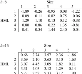
(9) data in the computation of pmv is bound to capture important variation in the market return’s sample path. Thus, pmvt. h;t. is simply de…ned as b2t b2t;t+h. =. for an aggregation level equal to h quarters.. 3.2. h X i=1. b2t+i. h;t ,. where. 1;t+i .. (2). Some preliminary evidence. Consistently with our discussion in Section 2, proper conditioning variables should have predictive ability for the moments of market returns. These moments may of course be highly nonlinear functions of the predictor(s), in general. De…ne market returns between t and t + h as Rt;t+h =. h j=1. 1 + Rt+ j. h. 1, where Rt+ j. h. is the j-th quarterly return on the market over horizon h. We regress Rt;t+h and b2t;t+h (or, equivalently, pmvt;t+h ) on pmvt. h;t .. We do so at various horizons and report results in Table. I. The regression of future market returns on pmv largely replicates …ndings in Bandi and Perron (2008) where risk premia (market returns in excess of the risk-free rate) are regressed on pmv : the predictive ability of pmv increases with the horizon. Not surprisingly, future market variance is best predicted by pmv at short horizons. This is an implication of the autoregressive nature of variance.. In the context of a traditional (in the existing literature) linear speci…cation, this evidence, and the related evidence in Bandi and Perron (2008), are meant to be merely suggestive of the informational content of pmv for the market return moments at various horizons. In what follows, we explore the cross-sectional pricing implications of this time-series predictability.. 4. Fama-French portfolio returns and pmv. In order to further motivate our approach, we now report the outcomes of regressions of the 25 Fama-French portfolio returns on pmv. In light of the countercyclical nature of …nancial market variance, our interest is largely on business-cycle frequencies. To this extent, we focus here on aggregation levels between 1 and 5 years. As earlier in the market case, we de…ne p portfolio returns between t and t + h as Rt;t+h =. h j=1. 1 + Rp. t+ hj. 1, where Rp. t+ hj. is the. j-th return on portfolio p over horizon h. We run the following regressions: p Rt;t+h =. p h. +. p h pmvt h;t. + "pt;t+h. h = 4; 8; 12; 16; 20. p = 1; 2; :::; 25.. (3). Table II contains the results. The betas of the 25 Fama-French portfolio returns with respect to pmv decrease in the size dimension (when going from small …rms to large …rms) and increase 7.

(10) in the value dimension (when going from low book-to-market stocks to high book-to-market stocks). In other words, at these frequencies, large …rms generally yield returns that are less correlated with pmv than small …rms. Similarly, value stocks yield returns that are more correlated with pmv than growth stocks. These patterns re‡ect similar patterns in average returns. As is well-known, average returns increase with value and decrease with size. As expected, they do so at all frequencies we consider. While these obvious structures in the betas are sometimes not fully monotonic, they are somewhat striking. When paired with the cross-sectional dispersion of average returns, they appear indicative of the cross-sectional pricing potential of pmv. We now turn to a more formal discussion of this issue. For a speci…c horizon h, write the fundamental pricing equation as p )]; 1 = Et [Mt+h (1 + Rt;t+h. (4). where Et denotes expectation conditional on time t information, Mt+h is the stochastic discount p factor, and Rt;t+h is, as earlier, the net return on the generic asset (portfolio, in our case) p.. Assume Mt+h = c1t + c2t ft;t+h , where ft;t+h is a factor. Classical models are the CAPM for which the factor ft;t+h is the market return over h and the C-CAPM for which ft;t+h is consumption growth over the same horizon. Even though, for reasons of economic generality and consistency with theory as laid out in Section 2, our interest in this paper is in the consumption speci…cation, in what follows we will report results pertaining to the CAPM case as well. In general, c1t and c2t are time-varying coe¢ cients whose dependence on time t macro variables depends on the true, unknown utility function.4 Write now c1t = a1 + a2 xt and c2t = b1 + b2 xt . In other words, assume that time-variation in the level and slope of the stochastic discount factor is driven by a variable x measurable with respect to time t information. This speci…cation, which could be readily extended to multiple states x, leads to p 1 = E[(a1 + a2 xt + b1 ft;t+h + b2 (xt ft;t+h )) (1 + Rt;t+h )];. with no need for a subscript t on the expectation operator. In other words, it leads to an unconditional multifactor beta speci…cation p et;h ] + E[Rt;t+h ] = E[R. 3 X. p h;i h;i ;. i=1. et;h ] is the expected return on the zero-beta portfolio uncorrelated with the stochastic where E[R discount factor (as in Black, 1972), the 4. p. s are multivariate betas of the returns on asset p on. In Campbell and Cochrane (1999), for example, c1t and c2t are functions of the "surplus consumption ratio.". 8.

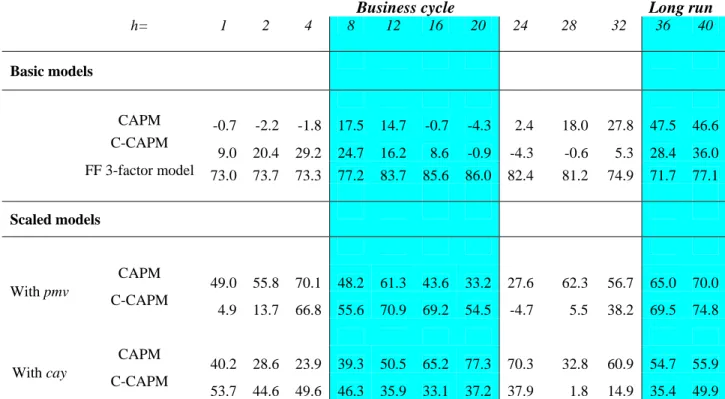
(11) xt , ft;t+h , and the interaction variable xt ft;t+h , and the s are the corresponding cross-sectional slopes.5 Assume now xt = pmvt h;t . When combined with the observed pattern in average portfolio b p ], the reported structure in the estimated pmv betas (obtained from Eq. (3) returns E[R t;t+h above) is suggestive of the potential economic and statistical signi…cance of the corresponding b estimate. Neglecting, but only for the time being, the additional loadings associated with the. factor ft;t+h and the interaction xt ft;t+h , this signi…cance is, in turn, indicative of the pricing potential of pmv as a scaling variable.. In what follows, we evaluate the cross-sectional relation between average returns and genuinely multivariate betas and its economic implications. Di¤erently put, we evaluate whether the level of historical market variance tracks meaningful predictable time-variation in the stochastic discount factor.. Conditional (on pmv) pricing. 5 5.1. Business-cycle frequencies. We employ a standard two-pass methodology for testing asset pricing models. For each asset p ) on f t;t+h = (xt ; ft;t+h ; p and horizon h, we …rst run a time-series regression of returns (Rt;t+h. xt ft;t+h )| , namely p Rt;t+h =. to estimate the loadings in the vector. p h. p | f t;t+h h. + p h:. + "pt;t+h ;. In the second step, for each horizon h, we run. cross-sectional regressions of the average returns on the portfolios on the estimated loadings to evaluate the resulting pricing errors: 1 T. h. T Xh t=1. p Rt;t+h. !. =. h. +. | ^p h h. + "h :. For the time being, we focus on two unconditional models, the CAPM and the C-CAPM, and their scaled versions (by pmv ). We report adjusted-R2 s (in Table III) and estimated lambdas (in Table IV) from the second-step, cross-sectional regressions. The adjusted-R2 values associated with the static CAPM and the static C-CAPM are, respectively, 17:5%; 14:7%;. 0:7%;. 4:3% and 24:7%; 16:2%; 8:6%;. 0:9%, at 2 to 5 years. Hence, market returns. and consumption growth perform similarly at these frequencies. Scaling by pmv improves the overall …t signi…cantly. The coe¢ cients of determination of the scaled models are 48:2%; 5. Since xt is not a risk factor, in conditional models the lambdas do not have a direct economic interpretation in terms of market prices of risk (see, e.g., the discussion in Cochrane, 1996, 2004, and Lettau and Ludvingson, 2001b). Similarly, of course, the betas do not have a direct interpretation in terms of quantities of risk. We discuss these issues in Section 8.. 9.

(12) 61:3%; 43:6%; 33:2% and 55:6%, 70:9%, 69:2%, 54:5%, thereby yielding a greater improvement in the C-CAPM case. Fig. 1 provides a graphical representation. The limitations of statistical metrics, such as coe¢ cients of determination, to evaluate pricing models are notorious. Section 8 focuses on economic signi…cance. As previously suggested, the betas associated with pmv play an important role (Table IV). This is especially true in the CAPM case where the lambdas associated with these betas have minimum t-statistics above 2:4 at business-cycle frequencies. In the C-CAPM case both the beta on pmv and the beta on the interaction matter at these frequencies. In particular, the estimated lambdas on the interaction have all t-statistics above 5:5. The lambdas on the market are negative but statistically insigni…cant. This is a typical result in the literature (see, e.g., the discussion in Lettau and Ludvigson, 2001b). The lambdas on consumption growth are instead positive and more statistically signi…cant. In spite of the lack of interpretability of the lambdas in terms of market prices of risk in conditional models, this result is generally more consistent with standard economic logic. Ignoring other terms, one would expect stocks delivering higher average returns to be riskier, as implied by their higher return correlations with consumption growth. This risk should be positively priced in equilibrium. For a clearer graphical assessment, Figs. 2 through 5 report the pricing errors associated with the static models (Fig. 2 and 4) and with the conditional models (Fig. 3 and 5). In particular, the values on the vertical axis are realized average returns on the portfolios, whereas the values on the horizontal axis are the corresponding …tted mean returns implied by each model (i.e., using estimated lambdas and betas). Naturally, if a model priced the portfolios exactly, the dots would sit on the 45 degree line. As always, for each value on the scatterplot, the …rst digit refers to the size quintile (with 1 indicating the smallest …rms and 5 indicating the largest …rms) and the second digit refers to the book-to-market quintile (with 1 indicating growth stocks and 5 indicating value stocks). The reduction in pricing errors yielded by pmv scaling is apparent.. 5.2. The long run. The adjusted-R2 values of the static CAPM and C-CAPM at 9 and 10 years are 47:5%, 46:6% and 28:4%, 36:0%, respectively. Therefore, the unconditional models perform somewhat better at low frequencies. In particular, market returns explain a larger portion of the cross-sectional variation of the Fama-French portfolios than consumption growth in the long run. Scaling by pmv increases the R2 -values to 65% and 70% in the CAPM case and to 69:5% and 74:8% in the C-CAPM case. The lambdas associated with the interaction are always positive and highly statistically signi…cant (Table IV). The lambdas associated with the pmv ’s. 10.

(13) loadings are also positive. They are signi…cant in the CAPM case and fairly insigni…cant in the C-CAPM case. While, in agreement with the static model, market returns play a more important role than consumption growth if considered individually, the joint consideration of the loadings with respect to the conditioning variable and the interaction yields smaller pricing errors in the C-CAPM case than in the CAPM case. When taking the theoretical implications of Section 2 seriously, since pmv strongly predicts long-run market returns as reported earlier (and extensively illustrated in Bandi and Perron, 2008), the improved …t delivered by pmv over the static C-CAPM should not be viewed as surprising. More generally, our …ndings suggest that pmv may contain meaningful information about time-variation in the stochastic discount factor both at business-cycle frequencies and at lower frequencies.. 6. Alternative pricing models. It is now informative to evaluate the pricing performance of scaled models using pmv as compared to existing successful alternatives, such as the classical Fama-French three-factor model and scaled speci…cations using cay. We begin with the latter. Lettau and Ludvigson (2001a) have shown that cay, coherently with its theoretical justi…cation,6 is a strong predictor of excess market returns at business-cycle frequencies. Table V supports this notion using our data. Consistent with its considerable predictive ability in the time series, Lettau and Ludvigson (2001b) have also shown that cay is a useful conditioning variable in scaled asset pricing models. We con…rm this result. At business-cycle frequencies the adjusted-R2 values yielded by cay in the CAPM case are 39:3%, 50:5%, 65:2%, and 77:3%. They are 46:3%, 35:9%, 33:1%, and 37:2% in the C-CAPM case. These values should of course be compared to the adjusted R2 -values of the static models in Table III and Fig. 1. When doing so, models scaled by cay are found to clearly dominate their unconditional counterparts. Interestingly, for our data, the pricing ability of pmv compares favorably to that of cay both at business-cycle frequencies and in the long run. Importantly, this is particularly true in the CCAPM case. This …nding may be appreciated by comparing adjusted-R2 s. More interestingly for our purposes, it may be appreciated by examining the nature of the conditional factor loadings implied by alternative scaling factors. Needless to say, this is a more compelling metric, for our purposes. Session 8 discusses conditional (on cay and pmv ) factor loadings for the C-CAPM. We show that, for our data, pmv leads to conditional consumption betas that are, in "bad states of the world," relatively more monotonically increasing with value and 6. A high value of the consumption-to-wealth ratio implies either expectations of high returns on wealth or expectations of low consumption growth.. 11.

(14) relatively more monotonically decreasing with size. Additionally, pmv leads to relatively larger spreads in the conditional consumption loadings than cay. Because the relevant notion of risk in conditional consumption models is covariation with consumption growth given the state of the economy, pmv appears to perform satisfactorily at explaining di¤erential average returns on portfolios by delivering risk quantities (i.e., conditional betas) which align fairly e¤ectively with these average returns. We conclude with the Fama-French three-factor model. As is well-known, the model uses the market returns, the returns on a "small minus big" (SMB) portfolio, and the returns on "high minus low" (HML) portfolio as the relevant factors.7 Hence, this speci…cation is genuinely multivariate. We …nd that this classical model performs extremely well at all frequencies, explaining over 70% of the cross-sectional variation of the returns on these portfolios. Table IV suggests that HML has prices of risk that are highly statistically signi…cant at virtually all frequencies (with the sole exception of the 9 and 10 year horizon). The contribution of the factor loadings associated with SMB and the market is instead reversed. SMB leads to prices of risk which are signi…cant (and positive) at high frequencies but are imprecisely estimated (and, eventually, negative) in the long run. The market returns yield risk prices which follow the opposite pattern. Hence, market risk plays a bigger role in the long run (as testi…ed by the higher value of the static CAPM at lower frequencies). The interpretation of the Fama-French factors is, to these days, controversial. The relation between Fama-French factors and undiversi…able macro risk has been the subject of some empirical investigation (see, e.g., Liew and Vassalou, 2000, inter alia) but no consensus has emerged. In light of the generally lower pricing errors delivered by the Fama-French model (at least when pricing size- and value-sorted portfolios), the success of recent consumption-based models8 should partly be viewed as a by-product of the Fama-French three-factor model being hard to interpret economically. Yet, arguably, this model represents an important benchmark. While, as typically found, we show that all scaled models yield larger pricing errors than the Fama-French model, scaling improves matters drastically.. 7. Addressing the critics. Lewellen and Nagel (2006) and Lewellen et al. (2007) have recently criticized the above two-step approach for testing pricing models on the 25 Fama-French portfolios. They claim that, since 7. The SMB portfolio is the di¤erence between the returns on small …rm portfolios and large …rm portfolios with the same book-to-market values. The HML portfolio is the di¤erence between the returns on high bookto-market …rm portfolios and low book-to-market …rm portfolios with the same size. We refer the reader to Kenneth French’s web site for details. 8 The "ultimate consumption" model of Parker and Julliard (2005), for instance, represents a promising alternative to scaled versions of the C-CAPM.. 12.

(15) these portfolios have a strong factor structure, the addition of factors, as e¤ectively implied by conditional models, is bound to spuriously in‡ate the explanatory power of the models being tested. To circumvent this issue, they make two main suggestions: expanding the set of test portfolios beyond the classical 25 Fama-French portfolios and using GLS, rather than OLS, in the second step of the traditional two-pass methodology. These approaches will lead to a more stringent test, but they remain subject to criticisms. For example, even if one takes the view that all assets should be priced by a valid pricing model, it is unclear why portfolios which do not have an obvious factor structure, like the industry portfolios, should provide a more compelling test than the 25 Fama-French portfolios. In a similar vein, GLS reshu- es the original portfolios and prices linear combinations of them, rather than the original portfolios, which are arguably of particular interest. Table VI contains the same information as in Table III, but instead of reporting adjustedR2 s;. we report R2 values when using GLS in the second step. In the implementation of GLS,. we employ the inverse of the unconditional covariance matrix of returns as the weight matrix. The …rst thing to notice is of course the much lower values of the R2 in this environment. Even the Fama-French three-factor model has a GLS R2 of 22% at 1 quarter compared with 73% for the OLS R2 . Scaling models by pmv leads to better …t than in the case of the unconditional models. This is true at all horizons. Importantly, no clear pattern across horizons seems to emerge relative to cay. Put it di¤erently, pmv remains competitive under this metric relative to a more sophisticated measure, such as cay. To increase the universe of portfolios, we add to our original 25 portfolios the 30 industry portfolios9 . The corresponding results are in Table VII. Once again, we notice that pmv improves the explanatory power of both CAPM and C-CAPM across all horizons, and particularly at business cycle frequencies and in the long run. The usefulness of pmv as a scaling variable relative to cay is apparent when comparing adjusted-R2 s: When examined based on the statistical …t of constructed portfolios (GLS portfolios) or portfolios with a mild factor structure (industry portfolios), well-known scaling variables, such as cay, may perform considerably less well. While the sense in which these portfolios represent a fully compelling test for conditional pricing models may be the object of some debate, pmv continues to fare well as compared to more-involved proxies even under alternative metrics. In the following section we use economic criteria based on implied conditional betas and conditional risk premia to assess the pricing relevance of pmv. We do so in the context of the original 25 Fama-French portfolios. 9. These are also available from Ken French’s web site.. 13.

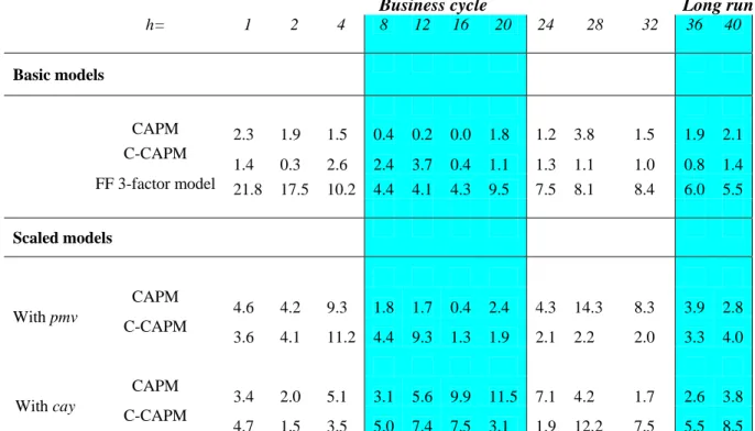
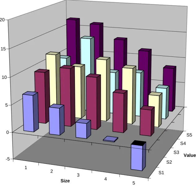
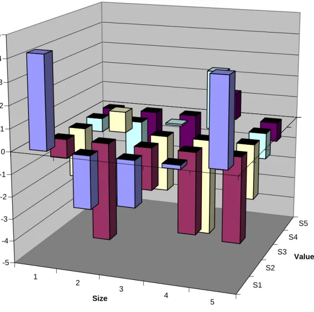
(16) 8. Conditional betas and risk premia. We focus on the C-CAPM. Table VIII reports betas on consumption growth, betas on pmv, as well as betas on the interaction at 4 levels of aggregations, i.e., 2, 3, 4, and 5 years. At all horizons, the average returns on the portfolios behave as described earlier, i.e., they decrease in the size dimension and increase in the value dimension. Lettau and Ludvigson’s logic justi…es this pattern (Lettau and Ludvigson, 2001b, Section II). In our scaled speci…cation, the correlation between portfolio returns and consumption growth is a function of the scaling factor. In other words, due to the interaction, the partial e¤ect of consumption growth on portfolio returns depends on the scaling variable, i.e., reports values of. p+ t. =. p. c+. p. + c;pmv pmvt h;t. where. p t. =. p. c+. pmvt+ h;t. p. c;pmv pmvt h;t .. Table VIII. is the mean of pmv conditional. on it being larger than 1 standard deviation above its mean. We de…ne. p t. in a similar fashion.. These de…nitions are the same as those in Lettau and Ludvigson (2001b). For small values of pmv the correlation between consumption growth and portfolio returns is generally small and often negative. It is large and positive for large values of pmv. Importantly, for large values of pmv, the correlation between portfolio returns and consumption growth increases in the value dimension and decreases in the size dimension, often almost monotonically. The spread in the conditional factor loadings is also substantial. Arguably, higher pmv values are associated with worse states of the world. Hence, value stocks require higher excess returns not because their unconditional risk (as measured by their unconditional beta with respect to consumption growth) is higher than for growth stocks. Rather, they appear to require higher excess returns because their conditional risk is higher in bad states (i.e., when pmv is higher). Lettau and Ludvigson (2001b) use this same logic to justify the role played by cay. Comparing our …ndings to the pricing ability of cay at the same horizons, in the case of pmv we generally …nd conditional (on bad states) consumption loadings that align more e¤ectively with historical average portfolio returns, more monotonicity in the conditional (on bad states) loadings, and larger di¤erences in the loadings between small/big …rms and low/high book-to-market …rms. Consider the 3 year horizon, for instance. Figures 6 and 7 depict these betas conditional on high and low pmv respectively. The low book-to-market/high book-to-market loadings associated with …rms in the …ve size quintiles are 6:7=16:6, 4:9=16:07, 2:73=13:36, 0:16=11:51, in the pmv case. They are 4:42=4:59,. 1:61=3:14,. 2:78=1:53,. 4:48=8:52. 2:88=5:22, 4:73=3:84 in the. case of cay. Similar …gures occur at alternative horizons (c.f., Table VIII). p. It is easy to show that, given conditional consumption loadings equal to t , the implied price et;h V art ( c)c2t , where c2t = b1 +b2 pmvt h;t . Asof consumption risk t can be expressed as R et;h (estimated from the cross-sectional regression) and a constant variance suming a constant R 14.

(17) of consumption growth,10 we evaluate. t. after estimating the coe¢ cients in c2t as recommended. by Cochrane (1996) and Lettau and Ludvigson (2001b), i.e., using the estimated cross-sectional s.. 9. Conclusions. In a world without risk, or with risk-neutral agents, prices are martingales and conditional expectations of future prices only depend on current prices. When risk is meaningful, prices are conditional expectations of future prices only after appropriate stochastic discounting. We conjecture that this stochastic risk correction is correlated with the level of past market variance (pmv ). In other words, we conjecture that past …nancial market variability proxies for more fundamental (and usually di¢ cult to measure) variables that may drive time-variation in the assessment of risk induced by macro factors, such as consumption growth. We test this conjecture by investigating the cross-sectional pricing of classical test assets, namely the Fama-French size- and value-sorted portfolios, using traditional asset pricing models scaled by the level of past market variance. The pricing ability of pmv is found to be substantial, particularly at business-cycle frequencies. When compared to variables that have been shown to be successful in the same classes of models (such as cay), pmv is found to fare very satisfactorily. 10. Both assumptions can be easily relaxed.. 15.

(18) References [1] Adrian, T. and J. Rosenberg, 2008. Stock returns and volatility: pricing the short-run and long-run components of market risk. Journal of Finance 63, 2997-3030. [2] Andersen, T.G., Bollerslev, T., Diebold, F.X., Labys, P., 2003. Modeling and forecasting realized volatility. Econometrica 71, 579-625. [3] Ang, A., Hodrick, R., Xing, Y., Zhang, X., 2006. The cross-section of volatility and expected returns. Journal of Finance 61, 259-299. [4] Bandi, F.M., Perron, B., 2008. Long-run risk-return trade-o¤s. Journal of Econometrics 143, 349-374. [5] Bandi, F.M., Moise, C., Russell, J.R., 2006. The joint pricing of volatility and liquidity. Working paper. [6] Black, F., 1972. Capital market equilibrium with restricted borrowing. Journal of Business 45, 444-455. [7] Barndor¤-Nielsen, O.E., Shephard, N., 2002. Econometric analysis of realized volatility and its use in estimating stochastic volatility models. Journal of the Royal Statistical Society, Series B 64, 253-280. [8] Campbell, J.Y., Cochrane, J.H., 1999. By force of habit: A consumption-based explanation of aggregate stock-market behavior. Journal of Political Economy 107, 205-251. [9] Cochrane, J.H., 1996. A cross-sectional test of an investment-based asset pricing model. Journal of Political Economy 104, 572-621. [10] Cochrane, J.H., 2004. Asset Pricing. Princeton: Princeton University Press. [11] Engle, R., Gonzalo, J., 2008. The spline GARCH model for low-frequency volatility and its global macroeconomic causes. Review of Financial Studies 21, 1187-1222. [12] Fama, E.F., French, K.R., 2002. The cross-section of expected returns. Journal of Finance 47, 427-465. [13] Fama, E.F., French, K.R., 2003. Common risk factors in the returns on stocks and bonds. Journal of Financial Economics 33, 3-56. [14] Lettau, M., Ludvigson, S.C., 2001a. Consumption, aggregate wealth, and expected stock returns. Journal of Finance 56, 815-849. 16.

(19) [15] Lettau, M., Ludvigson, S.C., 2001b. Resurrecting the (C-)CAPM: a cross-sectional test when risk premia are time-varying. Journal of Political Economy 109, 1238-1287. [16] Lettau, M., Wachter, J., 2007. Why is long-horizon equity less risky? A duration-based explanation of the value premium, Journal of Finance 62, 55-92. [17] Lewellen, J., Nagel, S., 2006. The conditional CAPM does not explain asset-pricing anomalies. Journal of Financial Economics 82, 289-314. [18] Lewellen, J., Nagel, S., Shanken, J., 2007. A Skeptical Appraisal of Asset-Pricing Tests. Working paper. [19] Liew, J., Vassalou, M., 2000. Can book-to-market, size, and momentum be risk factors that predict economic growth? Journal of Financial Economics 57, 221-245. [20] Moise, C., 2006. Stochastic volatility risk and the size anomaly. Working paper. [21] Parker, J., Julliard, C. 2005. Consumption risk and the cross-section of expected returns. Journal of Political Economy 113, 185-222. [22] Santos, T., Veronesi, P., 2006, Labor Income and Predictable Stock Returns. Review of Financial Studies 19, 1-44. [23] Spiegel, M., Wang, X., 2005. Cross-sectional variation in stock returns: liquidity and idiosyncratic risk. Working paper.. 17.

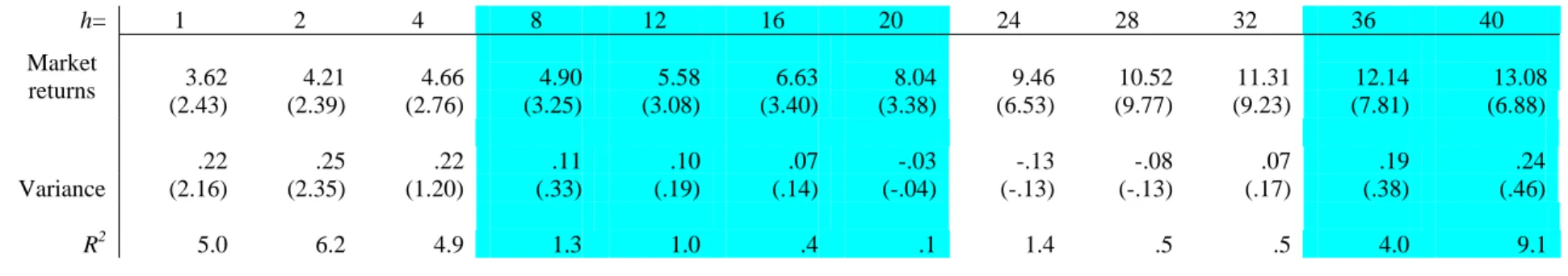
(20) Table I. Slope of forecasting regressions of market returns and market variance using pmv at different levels of aggregation h in quarters: 1952Q2-2006Q4 (t statistics in parentheses). h=. 1. 2. 4. 8. 12. 16. 20. 24. 28. 32. 36. 3.62 (2.43). 4.21 (2.39). 4.66 (2.76). 4.90 (3.25). 5.58 (3.08). 6.63 (3.40). 8.04 (3.38). 9.46 (6.53). 10.52 (9.77). 11.31 (9.23). 12.14 (7.81). 13.08 (6.88). Variance. .22 (2.16). .25 (2.35). .22 (1.20). .11 (.33). .10 (.19). .07 (.14). -.03 (-.04). -.13 (-.13). -.08 (-.13). .07 (.17). .19 (.38). .24 (.46). R2. 5.0. 6.2. 4.9. 1.3. 1.0. .4. .1. 1.4. .5. .5. 4.0. 9.1. Market returns. - 18 -. 40.

(21) Table II. Betas for univariate regressions of the 25 FF portfolio returns on pmv at levels of aggregation h (in quarters) 1952Q2-2006Q4. h=4. HML. 1 2 3 4 5. 1 2.44 3.02 3.13 2.92 2.91. 2 2.25 2.53 1.95 1.70 2.88. h=12. HML. 1 2 3 4 5. 1 -1.06 1.55 2.18 2.10 2.61. 1 2 3 4 5. 1 1.47 7.05 5.97 5.96 8.71. 2 0.74 0.42 2.51 2.52 1.21. h=20. HML. 2 6.15 5.83 7.47 7.96 5.44. Size 3 1.23 1.78 1.28 2.05 3.10. Size 3 0.90 2.01 1.47 1.45 3.03. Size 3 7.53 6.94 6.52 5.88 8.47. h=8 4 1.67 1.61 1.56 2.74 3.64. 5 0.72 1.59 0.33 1.02 1.33. HML. 1 2 3 4 5. 1 -1.89 0.09 1.29 0.80 0.41. 1 2 3 4 5. 1 0.68 3.69 3.07 3.31 5.27. 2 -0.26 0.11 1.10 0.86 0.54. h=16 4 0.86 1.35 0.69 1.45 2.40. 4 6.05 6.40 4.45 2.31 5.39. 5 -1.69 0.02 -0.63 -0.76 0.09. HML. 2 2.74 2.10 4.45 4.03 2.52. 5 1.30 5.62 3.11 3.27 5.84. - 19 -. Size 3 -0.95 0.82 0.13 0.22 1.44. Size 3 3.57 3.63 3.09 3.12 5.33. 4 0.08 0.75 0.12 1.35 2.40. 4 2.36 3.10 1.82 1.29 3.12. 5 -1.22 0.06 -0.38 -0.81 -0.04. 5 -1.86 1.63 0.11 0.14 1.90.

(22) Table III. Adjusted-R2 (%) from cross-sectional pricing regressions on the 25 FF size- and value-sorted portfolios at different levels of aggregation h (in quarters): 1952Q2-2006Q4. Business cycle. Long run. h=. 1. 2. 4. 8. 12. 16. 20. 24. 28. 32. 36. 40. CAPM C-CAPM. -0.7. -2.2. -1.8. 17.5. 14.7. -0.7. -4.3. 2.4. 18.0. 27.8. 47.5. 46.6. 9.0 73.0. 20.4 73.7. 29.2 73.3. 24.7 77.2. 16.2 83.7. 8.6 85.6. -0.9 86.0. -4.3 82.4. -0.6 81.2. 5.3 74.9. 28.4 71.7. 36.0 77.1. 49.0. 55.8. 70.1. 48.2. 61.3. 43.6. 33.2. 27.6. 62.3. 56.7. 65.0. 70.0. 4.9. 13.7. 66.8. 55.6. 70.9. 69.2. 54.5. -4.7. 5.5. 38.2. 69.5. 74.8. 40.2. 28.6. 23.9. 39.3. 50.5. 65.2. 77.3. 70.3. 32.8. 60.9. 54.7. 55.9. 53.7. 44.6. 49.6. 46.3. 35.9. 33.1. 37.2. 37.9. 1.8. 14.9. 35.4. 49.9. Basic models. FF 3-factor model Scaled models. CAPM With pmv. C-CAPM. CAPM With cay. C-CAPM. - 20 -.

(23) Table IV: Lambdas from cross-sectional pricing regressions on the 25 FF size- and value-sorted portfolios at different levels of aggregation h (in quarters): 1952Q2-2006Q4 (t-statistics in parentheses). Fama-French 3-factor model. h= 1 2 4 8 12 16 20 24 28 32 36 40. constant 5.06 (3.4) 5.54 (3.2) 5.86 (3.1) 1.97 (1.1) 1.59 (2.3) 2.23 (2.5) 2.16 (2.3) 2.48 (2.4) 2.41 (2.6) 1.84 (1.8) 1.26 (1.1) 1.02 (.9). market -1.83 (-1.3) -2.25 (-1.3) -2.47 (-1.4) 1.33 (.7) 1.75 (1.8) 1.31 (1.5) 1.65 (1.8) 1.70 (1.7) 2.11 (2.4) 3.09 (3.3) 4.01 (3.7) 4.65 (4.7). - 21 -. SMB 0.66 (2.4) 0.88 (2.6) 0.67 (2.4) 0.16 (.7) 0.24 (.12) 0.15 (.7) 0.03 (.12) -0.11 (-.5) -0.15 (-.5) -0.17 (-.5) -0.20 (-.6) -0.18 (-.6). HML 1.23 (5.0) 1.18 (3.9) 1.70 (6.2) 1.93 (5.1) 1.81 (4.8) 2.00 (5.1) 2.03 (4.8) 2.10 (4.3) 1.82 (3.4) 1.02 (2.0) 0.56 (1.1) 0.46 (1.1).

(24) Scaled CAPM Scaled by pmv h= 1 2 4 8 12 16 20 24 28 32 36 40. constant 5.13 (4.2) 2.59 (1.5) 3.07 (2.8) 4.45 (1.7) 4.75 (3.5) 3.67 (2.7) 2.62 (1.5) 0.00 (.0) 0.00 (.0) 0.37 (.3) 0.76 (.6) 0.86 (.7). market -1.64 (-1.4) 0.74 (.5) 0.33 (.3) -0.75 (-.3) -1.37 (-1.0) -0.01 (.0) 1.50 (.8) 4.39 (1.8) 4.89 (4.6) 4.53 (4.0) 4.43 (3.8) 4.85 (4.3). pmv 0.71 (2.9) 0.78 4.5) 0.41 (3.3) 0.55 (3.4) 0.53 (4.6) 0.39 (3.4) 0.28 (2.4) 0.14 (1.0) -0.05 (-.6) 0.13 (1.9) 0.18 (3.3) 0.16 (3.3). Scaled by cay pmv x market 0.43 (.2) 3.12 (1.6) 1.01 (.4) 7.06 (.7) 10.73 (1.1) 14.69 (1.2) 17.52 (1.0) 34.61 (1.4) 44.44 (2.4) 67.51 (3.1) 79.36 (3.0) 92.16 (3.4). - 22 -. constant 5.96 (5.1) 4.97 (3.7) 7.36 (3.5) 2.37 (.7) 3.21 (1.7) 2.78 (2.3) 2.73 (2.7) 3.52 (2.9) 2.10 (1.3) 1.90 (1.7) 1.83 (1.1) 2.44 (1.5). market -2.35 (-2.2) -1.38 (-1.2) -3.52 (-1.8) 1.25 (.4) 0.51 (.3) 1.03 (.8) 1.25 (1.2) 0.58 (.5) 3.01 (1.8) 3.63 (3.3) 4.51 (3.2) 4.58 (3.0). Cay -2.28 (-3.6) -0.98 (-2.1) -0.68 (-3.1) -0.29 (-3.8) -0.23 (-4.7) -0.18 (-5.2) -0.16 (-6.1) -0.15 (-4.4) -0.02 (-.4) 0.06 (2.5) 0.04 (1.9) 0.02 (1.3). cay x market -3.02 (-0.7) -0.72 (-.1) -6.40 (-1.6) -2.81 (-1.2) -5.03 (-2.7) -5.43 (-3.4) -6.98 (-4.4) -6.20 (-2.5) -4.69 (-1.2) -1.70 (-.5) -2.39 (-.5) -7.52 (-1.4).

(25) Scaled C-CAPM Scaled by pmv h= 1 2 4 8 12 16 20 24 28 32 36 40. constant 3.18 (5.9) 2.70 (3.7) 4.29 (9.6) 2.81 (6.8) 2.89 (11.9) 2.48 (7.9) 1.35 (1.9) 3.69 (2.5) 6.62 (5.5) 5.82 (6.3) 3.94 (4.6) 4.11 (4.3). consumption growth 0.43 (2.0) 0.25 (1.3) -0.02 (-.1) 0.26 (2.6) 0.14 (1.6) 0.18 (2.0) 0.15 (1.5) 0.05 (.3) -0.04 (-.2) 0.08 (.5) 0.09 (.7) 0.05 (.4). Scaled by cay pmv -0.10 (-.3) 0.06 (.2) 0.15 (1.0) 0.47 (3.0) 0.31 (2.5) 0.13 (1.2) 0.26 (2.6) 0.12 (.8) -0.13 (-1.0) -0.12 (-1.4) 0.05 (1.1) 0.12 (2.8). interaction 0.22 (.6) 0.26 (.4) -0.41 (-1.1) 2.80 (5.5) 2.74 (6.9) 2.92 (6.9) 4.25 (5.6) 1.91 (1.2) -1.06 (-.8) 1.33 (.8) 4.45 (2.9) 4.44 (2.9). - 23 -. constant 4.85 (4.9) 3.93 (3.4) 4.78 (4.0) 4.63 (5.4) 5.84 (8.2) 6.02 (10.8) 6.88 (10.8) 7.23 (7.7) 6.12 (5.1) 3.97 (3.5) 3.07 (2.5) 2.61 (2.0). consumption growth 0.21 (1.7) 0.24 (2.2) 0.27 (2.8) 0.20 (1.7) 0.17 (1.4) 0.12 (1.0) 0.02 (.2) -0.06 (-.6) -0.16 (-1.2) -0.22 (-1.7) -0.34 (-2.6) -0.30 (-2.4). cay -0.94 (-1.3) -0.29 (-.7) -0.34 (-1.7) -0.20 (-2.6) -0.19 (-3.3) -0.14 (-3.4) -0.14 (-3.8) -0.12 (-3.1) -0.06 (-1.3) 0.02 (.6) 0.00 (.1) 0.00 (.2). interaction 0.05 (.1) 0.03 (.1) -0.44 (-1.2) -0.41 (-1.3) -0.88 (-2.9) -0.97 (-3.0) -1.37 (-2.9) -1.39 (-2.4) -0.91 (-1.2) 0.52 (.8) 0.21 (.4) 0.25 (.5).

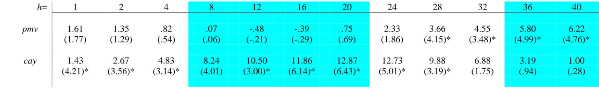
(26) Table V. Forecasting regressions of excess market returns using pmv and cay at different levels of aggregation h in quarters: 1952Q2-2006Q4. h=. 1. 2. 4. 8. 12. 16. 20. 24. 28. 32. 36. 40. pmv. 1.61 (1.77). 1.35 (1.29). .82 (.54). .07 (.06). -.48 (-.21). -.39 (-.29). .75 (.69). 2.33 (1.86). 3.66 (4.15)*. 4.55 (3.48)*. 5.80 (4.99)*. 6.22 (4.76)*. cay. 1.43 (4.21)*. 2.67 (3.56)*. 4.83 (3.14)*. 8.24 (4.01). 10.50 (3.00)*. 11.86 (6.14)*. 12.87 (6.43)*. 12.73 (5.01)*. 9.88 (3.19)*. 6.88 (1.75). 3.19 (.94). 1.00 (.28). - 24 -.

(27) Table VI. GLS R2 (%) from cross-sectional pricing regressions on the FF 25 size- and value-sorted portfolios at different horizons: 1952Q2-2006Q4 Weights given by the variance of returns Business cycle. Long run. h=. 1. 2. 4. 8. 12. 16. 20. 24. CAPM C-CAPM. 2.3. 1.9. 1.5. 0.4. 0.2. 0.0. 1.8. 1.2. 1.4 21.8. 0.3 17.5. 2.6 10.2. 2.4 4.4. 3.7 4.1. 0.4 4.3. 1.1 9.5. 4.6. 4.2. 9.3. 1.8. 1.7. 0.4. 3.6. 4.1. 11.2. 4.4. 9.3. 3.4. 2.0. 5.1. 3.1. 4.7. 1.5. 3.5. 5.0. 28. 32. 36. 40. 3.8. 1.5. 1.9. 2.1. 1.3 7.5. 1.1 8.1. 1.0 8.4. 0.8 6.0. 1.4 5.5. 2.4. 4.3. 14.3. 8.3. 3.9. 2.8. 1.3. 1.9. 2.1. 2.2. 2.0. 3.3. 4.0. 5.6. 9.9. 11.5. 7.1. 4.2. 1.7. 2.6. 3.8. 7.4. 7.5. 3.1. 1.9. 12.2. 7.5. 5.5. 8.5. Basic models. FF 3-factor model Scaled models. CAPM With pmv. C-CAPM. CAPM With cay. C-CAPM. - 25 -.

(28) Table VII. Adjusted-R2 (%) from cross-sectional pricing regressions on the FF 25 size- and value-sorted portfolios and 30 industry portfolios at different horizons: 1952Q2-2006Q4. Business cycle. Long run. h=. 1. 2. 4. 8. 12. 16. 20. 24. 28. 32. 36. 40. CAPM C-CAPM. 0.6. 1.4. -0.8. 1.3. -0.3. -0.3. -1.0. -1.7. -1.9. -0.9. 5.1. 5.5. 1.2 17.1. -0.1 14.7. -1.7 14.2. -1.2 20.1. 0.5 26.5. 1.4 38.3. 4.0 53.6. 9.6 58.4. 17.4 55.2. 21.4 48.1. 32.9 47.8. 31.7 47.0. 1.7. 13.0. 11.9. 9.2. 27.0. 36.3. 34.5. 21.9. 6.3. 10.4. 20.9. 28.3. 3.8. 14.4. 10.7. 18.7. 23.1. 16.3. 7.1. 12.1. 28.0. 33.2. 48.3. 50.0. 4.0. 7.5. 11.2. 6.0. 0.0. 1.5. 15.8. 42.6. 29.9. 4.5. 5.3. 2.8. 0.2. -0.3. 3.3. 5.0. 2.6. 4.8. 14.0. 29.6. 33.4. 39.2. 43.8. 44.3. Basic models. FF 3-factor model Scaled models. CAPM With pmv. C-CAPM. CAPM With cay. C-CAPM. - 26 -.

(29) Table VIII: C-CAPM betas and conditional betas (for low and high values of the state variable) with pmv and cay pmv - 2 year horizon Betas on consumption growth. HML. 1 2 3 4 5. 1 2.42 0.04 -0.96 1.11 0.24. 2 -2.72 -2.73 1.56 -1.95 -2.74. Betas on pmv. Size 3 -0.21 -1.80 -1.22 -0.21 -2.14. 4 -0.12 -2.58 -4.24 -0.37 -0.83. 5 4.73 -3.48 -2.08 -0.37 -1.34. HML. 1 2 3 4 5. 1 -4.71 -4.33 -3.38 -1.88 -5.09. Size 3 -2.74 -4.30 -4.79 -3.88 -5.03. 4 -1.63 -3.79 -7.01 -4.06 -3.88. 5 1.02 -4.87 -4.90 -4.31 -5.95. Size 3 0.25 -0.49 0.05 0.86 -0.47. 4 0.33 -1.43 -2.43 1.04 0.80. 5 4.22 -2.24 -0.93 0.55 0.19. 2 -5.02 -5.44 -1.73 -4.48 -7.58. Betas on the interaction. HML. 1 2 3 4 5. 1 0.84 1.25 1.30 0.77 1.56. 2 1.30 1.52 0.83 1.48 2.25. Size 3 0.50 1.42 1.37 1.16 1.80. 4 0.48 1.24 1.95 1.52 1.76. 5 -0.56 1.34 1.25 0.98 1.65. Conditional betas – high pmv 1. HML. 1 2 3 4 5. 9.17 10.12 9.56 7.36 12.80. 2 7.77 9.55 8.22 9.98 15.41. Conditional betas – low pmv Size 3 3.84 9.62 9.84 9.10 12.34. 4 3.78 7.44 11.47 11.91 13.38. 5 0.24 7.30 7.96 7.56 11.97. HML. 1 2 3 4 5. 1 3.20 1.20 0.25 1.83 1.69. 2 -1.51 -1.32 2.33 -0.58 -0.65. - 27 -.

(30) pmv - 3 year horizon. Betas on consumption growth. HML. 1 2 3 4 5. 1 3.62 -3.19 -5.46 -3.02 -4.85. 2 -3.98 -7.80 -1.06 -6.94 -6.55. Betas on pmv. Size 3 -3.13 -4.46 -5.65 -1.71 -5.28. 4 -0.26 -6.12 -7.60 1.38 -1.08. 5 5.75 -5.74 -4.36 -2.77 -2.98. 1 2 3 4 5. HML. 1 -1.31 -3.86 -5.38 -3.34 -6.36. 2 -3.44 -8.17 -1.71 -6.81 -8.56. Size 3 -1.98 -4.16 -6.15 -2.49 -5.00. 4 0.65 -4.94 -7.68 -0.77 -2.42. 5 3.40 -5.15 -5.39 -4.57 -4.80. Betas on the interaction. HML. 1 2 3 4 5. 1 0.29 1.21 1.63 1.23 2.04. 2 0.84 1.76 1.04 2.00 2.14. Size 3 0.55 1.33 1.64 0.92 1.76. 4 0.04 1.26 1.71 0.67 1.19. 5 -0.97 0.99 0.97 0.82 1.09. Conditional betas – pmv high. 1. HML. 1 2 3 4 5. 6.71 9.60 11.78 10.02 16.68. 2 4.91 10.75 9.90 14.21 16.07. Conditional betas – pmv low Size 3 2.73 9.60 11.63 8.04 13.36. 4 0.16 7.19 10.45 8.43 11.51. 5 -4.48 4.72 5.90 5.91 8.52. HML. 1 2 3 4 5. 1 4.18 -0.86 -2.31 -0.64 -0.93. 2 -2.36 -4.42 0.94 -3.08 -2.42. - 28 -. Size 3 -2.06 -1.90 -2.50 0.07 -1.88. 4 -0.18 -3.69 -4.31 2.67 1.22. 5 3.88 -3.83 -2.48 -1.18 -0.88.

(31) pmv - 4 year horizon Betas on consumption growth. HML. 1 2 3 4 5. 1 9.48 -1.82 -7.50 -4.24 -3.69. Betas on pmv Size 3 -3.21 -5.63 -6.86 -3.43 -5.34. 2 -2.53 -9.47 -2.02 -10.51 -6.86. 4. 5. 0.01 -7.81 -10.28 0.35 -3.52. 2.24 -10.10 -8.37 -6.22 -5.31. HML. 1 2 3 4 5. 1 6.09 -0.60 -6.93 -3.97 -3.53. 2 -0.21 -8.76 -1.77 -10.11 -8.01. Size 3 0.07 -4.29 -6.47 -3.68 -3.69. 4 2.47 -5.64 -10.15 -2.08 -4.78. 5 0.31 -9.05 -9.17 -7.73 -5.71. Betas on interaction. HML. 1 2 3 4 5. 1 -0.32 0.84 1.62 1.30 1.72. 2 0.45 1.62 1.28 2.30 1.81. Size 3 0.51 1.31 1.58 1.27 1.61. 4 -0.02 1.29 1.81 0.84 1.52. 5 -0.29 1.52 1.36 1.24 1.27. Conditional betas – pmv high. Conditional betas - pmv low Size. 1. HML. 1 2 3 4 5. 5.31 8.92 13.25 12.47 18.41. 2 3.19 11.37 14.34 19.01 16.35. Size 3 3.30 11.21 13.44 12.90 15.27. 4 -0.29 8.71 12.91 11.12 16.04. 5 -1.47 9.38 9.06 9.74 11.00. HML. 1 2 3 4 5. 1 8.50 0.69 -2.65 -0.34 1.48. - 29 -. 2 -1.19 -4.60 1.80 -3.61 -1.44. 3 -1.69 -1.70 -2.11 0.39 -0.52. 4 -0.06 -3.95 -4.86 2.87 1.05. 5 1.37 -5.55 -4.30 -2.49 -1.50.

(32) pmv - 5 year horizon. Betas on consumption growth. HML. 1 2 3 4 5. 1 16.12 4.66 -4.14 -0.20 5.07. Beta on pmv. 2 3.45 -5.36 3.30 -6.85 -0.52. Size 3 2.15 -2.28 -2.47 0.29 -2.83. 2 -0.13 1.03 0.75 1.66 0.90. Size 3 0.04 0.89 0.95 1.00 1.17. 4 2.21 -6.85 -8.79 0.86 -5.13. 5 -1.09 -12.56 -9.36 -7.57 -5.07. HML. 1 2 3 4 5. 1 14.76 9.82 -0.49 2.90 9.32. 2 8.76 -1.77 6.25 -3.26 1.29. Size 3 8.66 1.78 1.00 1.76 1.75. 4 7.40 -2.70 -7.20 -0.84 -5.09. 5 -1.35 -9.71 -8.77 -7.29 -2.85. Size 3 2.29 1.27 1.33 4.30 1.87. 4 2.19 -2.16 -2.81 4.30 1.81. 5 0.78 -5.23 -3.48 -1.92 0.23. Betas on interaction. HML. 1 2 3 4 5. 1 -0.85 0.00 0.93 0.69 0.57. 4 -0.01 1.17 1.49 0.86 1.73. 5 0.47 1.83 1.47 1.41 1.32. Conditional betas – pmv high. 1. HML. 1 2 3 4 5. 3.19 4.73 9.99 10.18 13.67. 2 1.53 10.20 14.62 18.35 13.09. Conditional betas – pmv low Size 3 2.69 11.15 11.88 15.45 14.95. 4 2.11 10.88 13.83 13.85 21.11. 5 5.99 15.14 12.88 13.79 14.98. HML. 1 2 3 4 5. 1 12.70 4.68 -0.40 2.54 7.34. - 30 -. 2 2.94 -1.25 6.30 -0.18 3.08.

(33) cay - 2 year horizon Betas on consumption growth. HML. 1 2 3 4 5. 1 5.88 4.62 3.70 4.22 6.21. 2 2.17 2.80 4.86 3.75 5.39. Betas on cay. Size 3 2.27 3.51 4.08 4.38 4.26. 4 1.82 2.29 2.90 5.19 5.60. 5 4.00 1.96 2.94 3.96 5.27. HML. 1 2 3 4 5. 1 5.73 7.64 2.43 2.86 0.18. 2 10.09 1.61 4.46 2.58 -1.68. Size 3 12.40 5.59 2.52 3.26 0.73. 4 15.56 3.72 0.36 2.42 -0.16. 5 14.04 4.87 4.09 1.98 4.93. Betas on the interaction. HML. 1 2 3 4 5. 1 0.42 -0.04 0.90 1.07 2.27. 2 -0.24 1.22 0.89 1.85 2.49. Size 3 -0.45 0.89 1.64 1.47 1.60. 4 -1.92 1.48 1.97 1.37 2.26. 5 -0.36 1.73 1.52 2.17 2.10. Conditional betas – cay high. 1. HML. 1 2 3 4 5. 6.76 4.54 5.56 6.43 10.91. 2 1.68 5.32 6.70 7.58 10.56. Conditional betas – cay low Size 3 1.33 5.35 7.47 7.43 7.58. 4 -2.16 5.36 6.98 8.03 10.28. 5 3.25 5.53 6.10 8.46 9.62. HML. 1 2 3 4 5. 1 5.05 4.70 1.92 2.10 1.70. 2 2.65 0.39 3.09 0.07 0.44. - 31 -. Size 3 3.16 1.74 0.83 1.45 1.08. 4 5.63 -0.64 -1.02 2.47 1.11. 5 4.72 -1.47 -0.09 -0.35 1.10.

(34) cay - 3 years horizon. Beta on consumption growth. HML. 1 2 3 4 5. 1 5.50 2.42 1.72 2.31 4.08. 2 0.48 0.68 3.36 2.14 3.31. Betas on cay. Size 3 0.13 1.71 2.01 2.54 2.30. 4 0.54 0.01 0.62 4.22 3.90. 5 2.72 -0.23 1.08 1.92 2.92. HML. 1 11.43 17.10 6.12 8.15 7.96. 1 2 3 4 5. 2 16.46 7.15 16.28 11.25 7.70. Size 3 20.87 15.01 8.88 12.04 9.34. 4 21.63 6.21 0.56 6.38 5.25. 5 13.98 5.38 4.74 4.12 14.26. Betas on the interaction. HML. 1 2 3 4 5. 1 -0.51 -1.63 -0.02 -0.33 0.24. 2 -0.97 -0.13 -1.38 -0.08 -0.08. Size 3 -1.36 -0.83 0.23 -0.59 -0.36. 4 -1.60 0.94 1.55 0.47 0.62. 5 0.94 1.78 1.58 1.64 0.43. Conditional betas – cay high. HML. 1 2 3 4 5. 1 4.42 -1.07 1.69 1.60 4.59. 2 -1.61 0.40 0.41 1.96 3.14. Conditional betas – cay low Size 3 -2.78 -0.06 2.50 1.28 1.53. 4 -2.88 2.02 3.94 5.22 5.22. 5 4.73 3.58 4.47 5.43 3.84. HML. 1 2 3 4 5. 1 6.53 5.72 1.75 2.98 3.60. - 32 -. 2 2.45 0.93 6.14 2.31 3.46. Size 3 2.88 3.37 1.54 3.73 3.03. 4 3.77 -1.90 -2.52 3.28 2.65. 5 0.82 -3.82 -2.12 -1.39 2.05.

(35) cay - 4 year horizon. Betas on consumption growth. HML. 1 2 3 4 5. 1 6.13 1.33 0.33 1.36 3.18. 2 -0.56 -0.53 3.08 1.28 2.29. Size 3 -0.91 0.68 1.14 2.36 1.38. Betas on cay. 4 -0.39 -1.24 -0.31 3.91 3.32. 5 2.20 -0.99 0.11 1.42 1.97. 1 2 3 4 5. HML. 1 12.43 15.81 -5.27 -1.36 9.01. 2 17.36 3.87 23.45 14.74 5.97. Size 3 27.73 17.37 11.49 14.28 13.35. 4 22.73 -0.10 -5.98 -0.10 4.14. 5 16.64 6.36 -1.91 4.96 25.63. Betas on the interaction. HML. 1 2 3 4 5. 1 -0.49 -0.95 1.47 0.82 -0.13. 2 -0.77 0.38 -1.95 -0.57 0.15. Size 3 -1.73 -0.89 -0.04 -0.87 -0.64. 4 -0.87 1.79 2.08 1.34 0.75. 5 1.22 1.72 2.46 1.61 -0.55. Conditional betas – cay high. HML. 1 2 3 4 5. 1 5.06 -0.74 3.54 3.16 2.90. 2 -2.25 0.30 -1.19 0.04 2.63. Conditional betas – cay low Size 3 -4.69 -1.28 1.05 0.46 -0.03. 4 -2.31 2.68 4.25 6.83 4.96. 5 4.86 2.78 5.51 4.93 0.76. HML. 1 2 3 4 5. 1 7.12 3.24 -2.63 -0.29 3.43. - 33 -. 2 1.00 -1.29 7.00 2.42 1.98. Size 3 2.56 2.48 1.22 4.11 2.68. 4 1.37 -4.84 -4.51 1.21 1.81. 5 -0.25 -4.45 -4.85 -1.82 3.09.

(36) cay - 5 year horizon. Betas on consumption growth. HML. 1 2 3 4 5. 1 5.68 -0.62 -2.08 -0.53 1.18. Size 3 -1.48 -0.62 -0.25 2.17 -0.67. 2 -1.08 -1.81 2.17 -0.67 0.95. Betas on cay. 4 -0.89 -2.16 -1.09 3.52 2.06. 5 2.24 -1.74 -0.29 0.66 1.21. HML. 1 2 3 4 5. 1 -14.58 -1.04 -29.01 -23.10 -8.46. 2 16.17 -6.14 16.74 4.30 -5.33. Size 3 33.87 10.98 9.07 12.98 5.58. 4 25.17 -3.14 -10.09 -7.56 -5.43. 5 27.82 16.15 2.96 10.54 40.31. Betas on the interaction. HML. 1 2 3 4 5. 1 2.59 1.24 3.61 3.02 1.70. 2 -0.10 1.49 -0.69 0.58 1.17. Size 3 -1.55 0.12 0.38 -0.49 0.32. 4 -0.30 1.99 2.08 1.95 1.65. 5 0.58 0.73 1.78 0.95 -1.57. Conditional betas – cay high. HML. 1 2 3 4 5. 1 11.42 2.14 5.93 6.18 4.95. 2 -1.31 1.48 0.64 0.60 3.55. Conditional betas – cay low Size 3 -4.92 -0.36 0.60 1.08 0.04. 4 -1.56 2.26 3.53 7.84 5.72. 5 3.54 -0.12 3.65 2.78 -2.27. HML. 1 2 3 4 5. 1 0.41 -3.16 -9.44 -6.69 -2.28. 2 -0.87 -4.84 3.57 -1.85 -1.45. - 34 -. Size 3 1.69 -0.86 -1.02 3.17 -1.33. 4 -0.29 -6.23 -5.34 -0.44 -1.31. 5 1.05 -3.23 -3.92 -1.28 4.40.

(37) Figure 1. Adjusted R2 in cross-sectional regression 90. 80. 70. 60. 50. 40. 30. 20. 10. 0 1. 4. 8. 12. 16. 20. 36. -10 Horizon (in quarters) CAPM. C-CAPM. CAPM-pmv. C-CAPM-pmv. CAPM-cay. C-CAPM-cay. 40.

(38) Figure 2. Realized vs. fitted returns on FF portfolios - CAPM Aggregation level = 12 Aggregation level = 8 7 15. Realized returns. 5. 24. 55. 54 42 5241. 5131. 3. 21. 2. 6. 2334 45 13 44 43 33 32 22. 12. 4. 15. 25 14 35 Realized returns. 6. 53. 55 51. 3. 3. 4. 5. 2. 6. Aggregation level = 16. 8. 4. 11. Fitted returns. 2. 24. 5. 2. 14. 25 35. 23 1334 45 44 12 43 3233 22. 53 54 52 41 42 3121. 3. 11. 4. 5. 6. Fitted returns. 7. Aggregation level = 40. 14. 15 15 14 25 35 24. 6. 23 1334 45 44 12 43 32 33 55 22 54 53 42 51 5241 3121 11. 5 4 3 2. 12 Realized returns. Realized returns. 7. 2. 3. 4. 5. Fitted returns. 2514. 10 44. 8. 7. 8. 6. 2 11 2. 45 34 13 23 32 33 12 55 22 54 52 53 42 4151. 43. 31. 4 6. 35 24. 21. 4. 6. 8. Fitted returns. 10. 12. 14.

(39) Figure 3. Realized vs. fitted returns on FF portfolios - CAPM scaled by pmv Aggregation level = 8 Aggregation level = 12 7 15. 34. 4.5 4. 22. 55. 3.5 31 51 21. 3 2.5. 15. 14. 25. 5 12 43 33 32. 54 53 41 52. 6. 35 24 23 44 45 13. 42. 2. 3. 5 43. 4. 4. 5. 2. 6. Aggregation level = 16. 22. 55. 2. 34 45 4412 32 33. 53 54 5241 31 21. 51 11. Fitted returns. 14. 25. 3. 11. 8. 3. 24 23. 35 13. 42. 4. 5. 6. Fitted returns. 7. Aggregation level = 40. 14. 15 15. 7 24. 5 4 51. 3 2. 2. 3. 35. 23 13 34 4445 12 4332 33 22 55 54 53 42 52 41 31 21 11. 4. 25. 14. 25. 6. 12 Realized returns. Realized returns. Realized returns. 5.5. Realized returns. 6. 5. Fitted returns. 6. 10 8. 43 55 33 54 52 53 51 4142. 6. 8. 2. 23. 13. 32 12 22. 31. 4 7. 45. 34 44. 1435 24. 21 11. 2. 4. 6. 8. Fitted returns. 10. 12. 14.

(40) Figure 4. Realized vs. fitted returns on FF portfolios - C-CAPM Aggregation level = 8 Aggregation level = 12 7 15 14. 5. 24. 4.5 4 3.5. 42 52 41 31 21. 3 2.5. 15 25. 6. 35. 34 23 13 45 1244 43 32 33 22 55 53 54. 2. 3. 14. 4. 5. Fitted returns. 5. 1334 23 45 44 43 12 3233 22 55 53 54 42 5241 51 3121. 4. 2. 6. Aggregation level = 16. 25. 35 24. 3. 51 11. 8. 2. 3. 4. 11. 5. 6. Fitted returns. 7. Aggregation level = 40. 14. 15 15. 7. 14 25 35 24. 6. 23 13 34 4544 12 43 32 33 22 55 54 42 53 52 41 51 3121. 5 4 3 2. 12. 2. 3. 4. 5. Fitted returns. Realized returns. Realized returns. Realized returns. 5.5. Realized returns. 6. 6. 10 34 44. 8. 7. 8. 2. 45 23. 13. 32 43 33 12 55 5422 52 51 41 53 42. 6. 31. 4. 11. 14 35 24. 25. 21 11. 2. 4. 6. 8. Fitted returns. 10. 12. 14.

(41) Figure 5. Realized vs. fitted returns on FF portfolios - C-CAPM scaled by pmv Aggregation level = 8. 24 34. 4.5. 12 43 33 32 22 55. 4 3.5 51 31. 3. 54 53 41 52. 7. 25 35. 6. Aggregation level = 12 15. 14. 5. 23 13. 45. 44. 42. 14. 5 4. 53 54 41 52 3121 11. 51. 3. 11. 2. 3. 4. 5. Fitted returns. 2. 6. Aggregation level = 16. 8. 25 2435. 34 1323 45 44 12 43 32 33 22 55 42. 21. 2.5. 2. 3. 4. 5. 6. Fitted returns. 7. Aggregation level = 40. 14. 15 15. 7 6 34 13. 5. 1244 43 32 33 22 55. 4 3 2. 51. 3. 25 35 24 23 45. 5354 5242. 41 31 21. 2. 12 Realized returns. 14 Realized returns. Realized returns. 5.5. 15. Realized returns. 6. 10 34 44. 8 6. 5. Fitted returns. 6. 7. 8. 2. 55 54 52 5341. 51. 24 45 23. 3514. 13. 43 33 1232 22. 42. 31. 4. 11. 4. 25. 21 11. 2. 4. 6. 8. Fitted returns. 10. 12. 14.

(42) Figure 6. Betas when pmv is high - 3 years. 20. 15. 10. 5. 0. S5 S4 S3. -5. S2 1. 2. 3 Size. S1 4. 5. Value.

(43) Figure 7. Betas when pmv is low - 3 years. 5 4 3 2 1 0 -1 -2 -3. S5 S4. -4 S3 -5. S2 1. 2. 3 Size. S1 4. 5. Value.

(44)