ÉCOLE DE TECHNOLOGIE SUPÉRIEURE UNIVERSITÉ DU QUÉBEC
THESIS PRESENTED TO
ÉCOLE DE TECHNOLOGIE SUPÉRIEURE
IN PARTIAL FULFILLMENT OF THE REQUIREMENTS FOR A MASTER’S DEGREE IN ELECTRICAL ENGINEERING
M. Eng.
BY
Zeynab MIRZADEH
MODELING THE FAULTY BEHAVIOUR OF DIGITAL DESIGNS USING A FEED FORWARD NEURAL NETWORK BASED APPROACH
MONTREAL, 19TH SEPTEMBRE, 2014
© Copyright reserved
It is forbidden to reproduce, save or share the content of this document either in whole or in parts. The reader who wishes to print or save this document on any media must first get the permission of the author.
BOARD OF EXAMINERS
THIS THESIS HAS BEEN EVALUATED BY THE FOLLOWING BOARD OF EXAMINERS
Mr. Jean-Francois Boland, Thesis Supervisor
Département de génie électrique à l’École de technologie supérieure Mr. Yvon Savaria, Thesis Co-supervisor
Département de génie électrique à l’École polytechnique de Montréal Mr. Christian Belleau, President of the Board of Examiners
Département de génie mécanique à l’École de technologie supérieure
Mr. Claude Thibeault, Member of the jury
Département de génie électrique à l’École de technologie supérieure
THIS THESIS WAS PRESENTED AND DEFENDED
IN THE PRESENCE OF A BOARD OF EXAMINERS AND PUBLIC 29 AUGUST 2014
FOREWORD
The Consortium for Research and Innovation in Aerospace in Québec (CRIAQ) is a non-profit consortium founded in 2002. It was established with the financial support of industry and university toward carrying out collaborative industry research projects at university. CRIAQ’s objectives are to improve knowledge of aerospace industry through education by training students in university. It improves competitiveness by enhancing knowledge on aerospace technology. ÉTS is involved in a number of CRIAQ projects and that project was carried as part of the CRIAQ AVIO403 project. The title of the AVIO403 project is Cosmic Radiation & Effect on Aircraft Systems. Bombardier Aerospace is the lead company involved in the project. Others partners in the project are MDA Corporation and the Canadian Space Agency. In addition, in this project, students and professors from the University of Montreal, École Polytechnique, Concordia, and the École de technologie supérieure are involved. The main objectives of the project are the development and validation of techniques and methodologies for verifying, testing and designing reliable systems subject to classes of radiations induced by cosmic rays.
ACKNOWLEDGMENTS
There are no proper words to convey my deep gratitude and respect for my thesis and research advisor, Professor Jean-Francois Boland. He taught me the skills to successfully formulate and approach a research problem. I would also like to thank him for being an open person to ideas, and for encouraging and helping me to shape my interest and ideas.
I would like to express my deep gratitude and respect to Professor Yvon Savaria, my co-supervisor whose advices and insight was invaluable to me. He generously provides me constructive criticism, which helped me develop a broader perspective to my thesis.
I would like to thank Marc-Andre Leonard, my teammate in AVIO403 project, who was involved in this project from the start and was a great support for everything. Thanks to him for questioning me about my ideas, helping me think rationally and even for hearing my problems.
I am most grateful to all member of AVIO403 project, especially Remi Robache who was involved in this project as a great help in running the experiments. He was highly responsible and cooperative with solving the problems about running the studies.
I would like to thank my family, especially my mother and father for always believing in me, for their continuous love and their supports in my decisions. Without them, I could not have made it here.
Thanks to my supportive friends in LACIME laboratory, Parisa, Sara, Hossein, Aria, Hassan, Fanny, Mathieu, Normand, Smarjeet and others who made the lab a friendly environment for working.
MODÉLISATION DU COMPORTEMENT FAUTIF DE CIRCUITS NUMÉRIQUES BASÉE SUR L’APPROCHE PAR RÉSEAUX DE NEURONES DE TYPE
CONNECTION-DIRECTE
Zeynab MIRZADEH
RÉSUMÉ
Les rayons cosmiques sont une source d’erreurs douces pour les circuits numériques. Dans le domaine aéronautique, aux altitudes des aéronefs, le flux de neutrons provenant des radiations cosmiques est plus élevé qu’au niveau de la mer. Il est donc utile d’étudier le comportement fautif d’un circuit avant son implémentation afin d’analyser sa robustesse en présence de pannes. Le but de cette recherche consiste à développer une approche pour la modélisation du comportement fautif des circuits numériques. Cette approche peut être appliquée tôt dans le flot de conception avant l’étape de fabrication. Pour ce faire, nous devons tout d’abord extraire le comportement fautif du circuit à partir d’un modèle décrit à bas niveau en langage HDL. Ensuite, cette information est utilisée pour la phase apprentissage d’un réseau de neurones décrit en langage C/C++ ou MATLABTM. Le modèle résultant servira à reproduire le comportement fautif du circuit en présence de pannes. Cette approche est propice à un développement d’une bibliothèque basée sur des modèles fautifs représentés par un réseau de neurones. Cette bibliothèque serait utilisée au niveau Matlab/Simulink et pourrait regrouper plusieurs classes de circuits. L’analyse de fiabilité devient donc possible à haut niveau et l’étude complète d’un design comprenant des sous-modules préalablement caractérisés est à la portée du concepteur.
La méthodologie développée dans le cadre de ce mémoire est basée sur des expérimentations effectuées sur deux circuits. Le premier est le ISCAS C17 avec lequel le comportement fautif a été généralisé par un réseau de neurones. Afin de valider notre méthodologie, les résultats ont été comparés avec une méthode préalablement développée basée sur génération de signatures. Par la suite, un multiplieur 4-bit est utilisé comme deuxième circuit plus élaboré. Les résultats de la modélisation du comportement fautif par réseaux de neurones montrent que la précision est augmentée comparativement à la méthode de génération de signatures. Pour le circuit C17, même en ne prenant que 30% des données générées par le simulateur de pannes LIFTING, le réseau de neurones est capable de reproduire le comportement fautif du circuit tout en préservant une erreur de modélisation sous les 6%.
Mots clés: SEU, réseau de neurones, comportement fautif, circuit numérique, C++,
MODELING THE FAULTY BEHAVIOUR OF DIGITAL DESIGNS USING A FEED FORWARD NEURAL NETWORK BASED APPROACH
Zeynab MIRZADEH
ABSTRACT
Cosmic rays lead to soft errors in electronic circuits. In avionic systems it is more critical, as the neutron flux that is caused by cosmic rays is stronger at high altitudes. It would be helpful to study the faulty behaviour of digital circuits before implementation to analyze their robustness in presence of faults. The goal of this research is to develop an approach for modeling the faulty behaviour of digital circuits. This proposed approach could be applied in a design flow before circuit fabrication to characterize the faulty behaviour of circuits for their early validation. This is achieved by extracting information about faulty behaviour of circuits from low-level models expressed in VHDL language. Afterwards the extracted information is used to train high-level artificial neural networks models expressed in C/C++ or MATLABTM languages. The trained neural network becomes a model able to replicate the faulty behaviour of the circuit in presence of faults. Later, trained artificial neural network models could be used to develop a components characterization library available in Matlab/Simulink regrouping different classes of circuits. These pre-defined faulty component models could also be used in high-level models to conduct reliability analysis. Thus, the faulty behaviour of each sub-circuit and their effects on a system could be assessed.
The methodology adopted in this thesis is based on experiments done with two important benchmarks. First, the faulty behaviour of the C17 ISCAS circuit is modeled using a neural network approach. To validate our method, the results are compared with a previously reported faulty signature generation method. Then, our proposed technique is tested with a 4 bit multiplier design, which has a larger dataset. Results show that the neural network approach leads to models that are more accurate than the signature generation method. For the circuit C17, by taking only 30% of the dataset generated with the LIFTING fault simulator, the neural network is able to replicate the output of the circuit in presence of faults while keeping the mean absolute modeling error below 6%.
TABLE OF CONTENTS
Page
INTRODUCTION ...1
CHAPITRE 1 LITERATURE REVIEW ...5
1.1 Cosmic rays in the earth atmosphere ...5
1.1.1 Effect of energetic neutrons on integrated circuits ... 7
1.1.2 Effectiveness of a shield ... 9
1.2 Faults caused by cosmic rays in digital systems ...10
1.2.1 Classification of faults caused by cosmic rays ... 10
1.2.2 Faults, errors and failures ... 12
1.3 Digital circuit verification by fault injection ...13
1.3.1 Fault models ... 14
1.3.1.1 Stuck-at (s-a) fault model ... 14
1.3.1.2 Bit flip fault model ... 15
1.3.2 Fault injection techniques ... 15
1.3.2.1 Hardware-based injection techniques ... 16
1.3.2.2 Emulation-based injection techniques ... 16
1.3.2.3 Simulation-based injection techniques ... 17
1.4 Developing fault behavioural model ...18
1.5 Neural network and fault ...19
1.6 Conclusion ...21
CHAPITRE 2 NEURAL NETWORKS AND THEIR APPLICATIONS IN FAULT MODELS ...23
2.1 A brief introduction to artificial neural network ...23
2.2 The neuron ...25
2.3 Neural network architectures ...28
2.4 Multi-layer perceptron (MLP) networks ...29
2.4.1 Preliminaries definitions for MLP learning algorithm explanation ... 31
2.4.1 MLP learning algorithm description ... 32
2.4.2 Neuronal activation functions ... 35
2.5 Multi-layer perceptron in practice ...38
2.5.1 Data preparation ... 38
2.5.2 Size of training data ... 38
2.5.3 Number of hidden layers ... 39
2.5.4 Generalization and over-fitting ... 39
2.5.5 Training, testing, and validation ... 40
2.5.6 When to stop learning ... 41
2.5.7 Computing and evaluating the results ... 42
CHAPITRE 3 PROPOSED METHODOLOGY ... 43
3.1 Neural network approach and different scenarios ... 43
3.1.1 Concept of signature ... 44
3.1.2 Scenario 1: signature adjustment ... 46
3.1.3 Scenario 2: faulty output prediction ... 47
3.2 Proposal to use neural network for predicting faulty output of circuits ... 48
3.2.1 Dataset generation ... 51
3.2.2 Neural network training phase ... 52
3.2.3 Neural network validation ... 53
3.2.4 Using the trained neural network ... 54
3.3 Conclusion ... 55
CHAPITRE 4 IMPLEMENTATION OF PROPOSED MODEL ... 57
4.1 Dataset generation ... 57
4.2 MLP Neural network in MATLABTM environment ... 58
4.3 MLP Neural network and OpenCV library written in C++ language ... 60
4.3.1 Parameters configuration ... 61
4.3.2 Layers definition ... 62
4.3.3 Network training ... 63
4.4 Case study for circuit C17 ... 63
4.5 Data sampling method for training neural network ... 65
4.5.1 Method of computation of errors ... 72
4.6 Neural network model for C17 in C++ environment ... 77
4.7 Results for a Multiplier circuit ... 78
4.8 Conclusion ... 82
CONCLUSION AND FUTURE WORK ... 83
APPENDIX I C++ CODE FOR CIRCUIT C17 USING OPENCV ... 85
LIST OF TABLES
Page Table 3.1 Computing error type for a circuit with following golden and faulty
outputs ...45
Table 3.2 Computing signatures for the arbitrary circuit presented in table 3.1 ...45
Table 4.1 Fault truth table for circuit C17. First 17 Injected fault fields show stuck-at-0 for all 17 different fault sites and second 17 injected fault fields show stuck-at-1 for all ...64
Table 4.2 Errors of evaluation of the neural network model for C17 while using different percentages of sampling of the 1088 number of data ...67
Table 4.3 Errors of evaluation of the neural network based model for circuit C17 with sample sizes less than 10% of the 1088 number of data ...69
Table 4.4 Comparison between the errors of the neural network based model and model proposed by (ROBACHE 2013) for C17 circuit ...70
Table 4.5 Error types for circuit C17 ...73
Table 4.6 Matrix of for circuit C17 ...76
Table 4.7 Matrix of for circuit C17 while percentage of sampling is 70% ...76
Table 4.8 Comparison of speed between MATLABTM and C++ environment ...78
Table 4.9 Errors of evaluation of the neural network model for circuit 4 bit multiplier while using different percentages of sampling of the 82688 number of data ...79
LIST OF FIGURES
Page
Figure 1.1 Neutron flux at different altitude ...6
Figure 1.2 Neutron flux in different latitude and altitude ...7
Figure 1.3 The high-energy neutron strikes the silicon atoms of a CMOS NPN transistor and a trail of electron-hole pairs are created as a result of this interaction ...8
Figure 1.4 Mitigation of the neutron flux as a function of the thickness of concrete in cm ...9
Figure 1.5 Fault classification based on cause and effect ...11
Figure 1.6 a) Fault which is masked in inner scope b) Fault which manifests in outer scope will be called error ...12
Figure 1.7 The fault s-a-0 is activated on line G when logic value 0 is applied on line G Adapted from Patel (2005) ...14
Figure 1.8 The bit flip fault injected into memory ...15
Figure 1.9 Classification of fault injection techniques ...18
Figure 2.1 A small example of an MLP neural network with one hidden layer ...25
Figure 2.2 A simple element which is called artificial neuron or perceptron. 1, 2, 3 and are neurons or perceptrons; The weights on the links to neuron from neurons 1, 2 and 3 are 1, 2 and 3 ...26
Figure 2.3 The sigmoid activation function ...27
Figure 2.4 The different architectures for neural network: a) single layer feed forward, b) multi-layer perceptron feed forward, c) recurrent network ...28
Figure 2.5 The multilayer perceptron neural network structure ...30
Figure 2.6 Steps of Multi-Layer Perceptron training algorithm ...33
Figure 2.7 Commonly used activation functions for a neuron, where O/P denotes the output of the neuron and I/P denotes the input ...37 Figure 2.8 There are two data sets. White ones are training data and red ones are
comes from the functions which are trained by the neural network. The left neural network has the ability of generalization but the right
neural network exhibits over fitting. ... 40
Figure 2.9 Mean-square error during training ... 41
Figure 3.1 Proposed sketch for scenario 1 to adjust signatures ... 47
Figure 3.2 Diagram of the proposed approach to mimic the behaviour of a combinational circuit in the presence of faults ... 48
Figure 3.3 The flow diagram to develop a Neural Network model which is able to predict faulty output of circuit ... 50
Figure 3.4 The flow diagram to show the steps to generate the training dataset and ... 51
Figure 3.5 Flow diagram to show the training phase of the neural network ... 52
Figure 3.6 Flow diagram for validation phase of neural network ... 54
Figure 3.7 Flow diagram for using phase of neural network ... 55
Figure 4.1 Fault sites specified for circuit C17 ... 58
Figure 4.2 Neural network based model for circuit C17 ... 65
Figure 4.3 Graphs of a) Error_category1, b) Error_category2, c) Error_category3 and d) mean_correlation coefficient ... 72
Figure 4.4 Graphs of a) Error_category1, b) Error_category2, c) Error_category3 and d) mean_correlation coefficient ... 82
LIST OF ABREVIATIONS
CMOS Complementary Metal-Oxide-Semiconductor
FPGA Field Programmable Gate Array
HDL Hardware Description Language
LUT Look Up Table
MTBF Mean Time Between Failures
SEU Single Event Upset
VHDL VHSIC Hardware Description Language
SEE Single Event Effect
SEL Single Event Latch up
SEFI Single Event Functional Interrupt
SET Single Event Transient
RHA Radiation Hardness Assurance
RBF Radial Basis Function
S-a Stuck-at
IC Integrated Circuit
ANN Artificial Neural Network
INTRODUCTION
FPGA-based circuits are very well-known in all fields of industry, including space, avionic and ground-level electrical instruments. For critical purposes, the reliability of such circuits is a primary concern. Therefore, the phenomena causing faults in circuits should be studied to ensure that measures are implemented to protect the system against these faults. One such class of phenomena is the single-event-upsets in flip-flops or memory cells. Neutrons are generated when cosmic particles strike nitrogen or oxygen atoms while travelling extremely fast in the upper layers of the atmosphere. When these neutrons hit silicon atom nucleus, they can generate secondary particles. Some of these particles are charged and they can generate trails of electron-hole pairs of a few microns in length. If one such trail is near a reversed-biased pn junction in a transistor, a voltage spike can be generated. Such a voltage spike can change the state of a memory cell or flip-flop. This state change is called a single-event-upset or soft error (Actel 2002). Before, this error was mainly considered in the space industry, but with the decreasing size of transistors, even ground-level instruments are susceptible to such problems. Though more robust FPGAs may be used (Brogley 2009), their price compared to traditional FPGAs makes them unaffordable in many applications. An optimized solution to this problem is to use traditional FPGAs with a new strategy for circuit design to improve their robustness.
Cosmic rays and their effects are known to upset electrical instruments in avionic circuits as well as those at the ground level notably because of the decreasing size of transistor (Ostler, Caffrey et al. 2009). They change the state of flip-flops in integrated circuits leading to soft errors. Consequently, circuits behave differently in the presence of such faults. For verifying the reliability of circuits before production, it would be helpful to know about the faulty behaviour of circuits.
To augment the sensitivity of electrical devices in avionic circuits, improvement of their robustness becomes necessary. In addition, radiation tolerant integrated circuits are often unaffordable and therefore robustness of traditional integrated circuits has to be increased by
implementing necessary mitigation strategies. This would enable their use in lieu of more expensive alternatives (Laura Dominik 2008).
Studying current methodologies to design circuits should be done so that old strategies could be adapted to formulate new ones that answer the requirements mentioned above. Thus, reliability requirements to protect avionic circuits could be specified during the design steps in order to obtain reliable inexpensive integrated circuits.
The main objective of this project is to develop a faulty behaviour model for FPGA-based circuits described at a high-level of abstraction. By using neural networks, fault behaviour models are developed and their accuracy is validated. The developed models could be used to replace any component of the entire circuit with faulty versions of the components described at a high-level of abstraction. This ensures that the effect of faulty behaviour of each component on a system could be analyzed at a high-level of abstraction and the mitigation technique could be used to improve the robustness of more critical parts. The steps proposed in this project are part of the CRIAQ AVIO403 project. Sub-objectives of the present master project are explained below:
• The first sub-objective is to emulate faults in models described at a high-level of abstraction. Therefore, a suitable fault injection method is proposed;
• The second sub-objective is to explore if the type of faulty behaviour modeling that is the goal of the project could be done with neural networks. There are several possible tasks: for example, a neural network could be developed to produce the faulty output of a circuit, or to predict the probability of occurrence of faults for each bit of the circuit output;
• The third sub-objective is to develop the faulty behaviour model of different circuit components, such as multiplier and adder, using the neural network structure proposed in the previous sub-objective;
• The last sub-objective is to develop a library of faulty behaviour blocks of the circuit components composing a Simulink model. Therefore, each time designers need to
analyse possible faulty behaviour of a circuit at a high-level of abstraction, the library of components could be used.
Contributions
This research proposes a fault behaviour model developed with a neural network concept in a novel way. The neural network structure is used to synthesize the faulty output of a circuit at a high-level of abstraction. All the strategies that are proposed in this research have novelty; and effort is exercised to find an appropriate structure for the neural network in this project.
Existing fault behaviour models for emulating faulty behaviour of circuits are not accurate enough and neural networks are proposed to enhance these models. This ensures a greater prediction accuracy while emulating faulty behaviour of avionic components.
Outline of the thesis
In the first chapter, the literature review is presented, and also the essential knowledge for understanding this thesis is summarized. Details about the nature of cosmic rays and their effects on avionic circuits are provided. Different effects cause different errors and faults in the circuit, and this is described and classified. Different tools for fault injection at different levels of abstraction are also verified.
In the second chapter, the concept of artificial neural network is explained. Different structures of neural networks are classified and training algorithms are explained. The training algorithm selected for the work presented here is explained in greater detail, including the reason behind its selection.
In the third chapter, different paths followed to develop a possible solution for the stated problem are described. This chapter also includes a detailed description of the scenario implemented here. Note that there are several scenarios to solve this problem. Signature generation and signature improvement are considered and explained in further detail.
In chapter four, all the steps for signature generation scenario are analysed in detail. We introduce new concepts for modeling fault behaviour using neural network based signatures. These concepts are analysed through several case studies.
The fifth chapter compares the results of this study with the results obtained by colleagues, whose work strategies and related limitations are specified. This comparison highlights the advantages and disadvantages of the approaches explored by the research team.
The conclusion chapter presents the results of the methodology adopted in this thesis, and also offers suggestions for possible opportunities of future work in this area of research.
CHAPITRE 1 LITERATURE REVIEW
In this chapter, cosmic rays and their effect on electronic circuits are explained. Cosmic rays are first described and then their effects on integrated circuits are studied. The classification of failures caused by cosmic rays is explained, and the difference between a fault and an error is defined. At the end, neural network is introduced in terms of its utility as a tool for detection and classification of faults in digital and analog circuits.
1.1 Cosmic rays in the earth atmosphere
Galactic cosmic rays and solar rays trace their origins to deep space and the sun. As they approach the earth, they collide with gas atoms in the upper atmosphere, like those of oxygen and nitrogen. As a result of these collisions, oxygen and nitrogen atoms disintegrate into a variety of high energy particles. Most of these particles recombine quickly. Neutrons constitute the main proportion of the product of these atmospheric collisions. These neutrons tend not to recombine and are projected from the collisions at very high rates. They travel at a high speed until a second collision occurs; such a second collision could be with oxygen or nitrogen atoms in atmosphere, objects traveling in atmosphere or objects on the earth’s surface (Velazco, Fouillat et al. 2007).
The amount of neutrons, which is called neutron flux, depends on the following factors (Actel 2002):
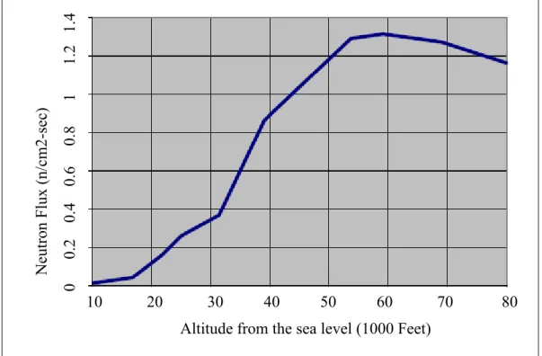
Altitude: At low altitudes, neutron flux decreases. Altitude is a significant factor affecting
Altitude from the sea level (1000 Feet) Ne ut ron Fl ux (n/c m2-se c) 10 20 30 40 50 60 70 80 0 0.2 0.4 0.6 0.8 1 1.2 1.4
Figure 1.1 Neutron flux at different altitude Adapted from Actel (2002)
Latitude: The earth’s magnetic field lines are closer together at the poles and hence facilitate
a greater trapping of cosmic particles than at the equatorial latitude. In figure 1.2, neutron flux variation with latitude and altitude is illustrated;
Figure 1.2 Neutron flux in different latitude and altitude Adapted from Actel (2002)
Longitude: It has some effects on the amount of cosmic rays but these effects are negligible
compared to the previously mentioned factors.
As explained, altitude is a significant factor affecting the neutron flux. At aircraft altitude, the amount of cosmic rays is more than ground level. With respect to latitude, the amount of cosmic rays is significantly more at the polar latitude than at the equator. Longitude plays an insignificant role, and its effect is negligible compared to the other factors affecting neutron flux.
In the next section, the effect of cosmic rays on electronic circuits is explained. The importance of these studies for avionic circuits is more considering that the effect of cosmic rays at airplane flying altitudes is significantly harsher than at the sea level.
1.1.1 Effect of energetic neutrons on integrated circuits
Nowadays, the effect of cosmic rays on electronic systems is well known. Neutrons are the main cause for such effects (Normand 1996). Neutrons produced by collisions travel at
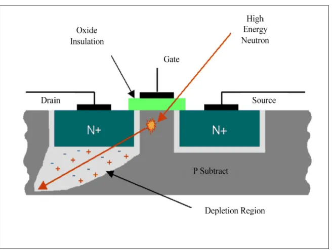
extremely high speed and can strike integrated circuits contained in avionic systems. Most of them will pass through integrated circuits without interacting with them. However, there are some neutrons that will pass close enough to a dopant or silicon atom, resulting in an impact. As a result of this disturbance, secondary particles are produced, creating a trail of electron-hole pairs. In figure 1.3, we see a transverse cut of a CMOS NPN transistor. When a high energy neutron strikes the silicon atoms, a trail of electron-hole pairs are created as a result of this interaction (Actel 2002).
Figure 1.3 The high-energy neutron strikes the silicon atoms of a CMOS NPN transistor and a trail of electron-hole pairs are created as a result of this interaction
Adapted from Actel (2002)
If the interaction happens near a reversed biased junction in a flip-flop or memory cell, a voltage spike could result. This effect could change the state of a memory element from zero to one or vice versa. This change is called single event upset (SEU). When only the state is
changed without any damage to the circuit, it is called a soft error. In the event of soft errors, the correct device operation may be restored by rewriting the memory element with the correct value.
The way in which circuits could be protected against high energy neutrons is by using shields, and is explained in the following section.
1.1.2 Effectiveness of a shield
It is very difficult to achieve an anti-neutron shield. In fact, even a thick concrete wall is not effective in reducing a neutron flux. The neutrons are slowed down and then absorbed by light nuclei. A material that contains hydrogen - such as water, polyethylene, paraffin, or concrete - is the best solution to mitigate such radiation. To do this effectively required a substantial thickness of material when neutron flux is high.
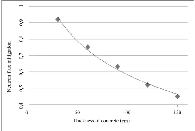
Figure 1.4 Mitigation of the neutron flux as a function of the thickness of concrete in cm Adapted from Dirk, Nelson et al. (2003)
Figure 1.4 represents the mitigation of the neutron flux as a function of the thickness of concrete as a shield. To reduce the flux to half, concrete with 1.3 m thickness should be used but providing such a thickness is very difficult in case of a lot of applications (Dirk, Nelson et al. 2003).
1.2 Faults caused by cosmic rays in digital systems
One way to measure the effect of cosmic rays on a digital system is to measure the soft error rate (SER). SER is the rate at which a system expected to encounter soft errors (Vibishna, Beenamole et al. 2013). In the study by Taber and Normand in 1993, the soft error rate (SER) in a large amount of SRAM CMOS systems was 1.2 ∗ 10 soft fails per bit per day at 9 km altitude (Taber and Normand 1993). In the Rosetta project (Lesea, Drimer et al. 2005), implemented by Xilinx, the effect of cosmic ray on FPGAs in different positions from the earth is illustrated. For this project, 100 groups of different FPGA technologies were placed at different altitudes from the earth surface. They were tested to collect data to measure the effect of cosmic rays. It was found that at higher altitude, the effect of cosmic rays is more and therefore FPGA based avionic circuits will be more vulnerable to the presence of cosmic rays. In the following section, different faults caused by cosmic rays are classified.
1.2.1 Classification of faults caused by cosmic rays
Faults are grouped into two main categories: non-recoverable and recoverable. Non-recoverable faults are the ones caused by cosmic rays with a destructive effect, whereas recoverable faults are those caused by cosmic rays without a destructive effect. For example, a faulty system can sometimes be fixed by reconfiguring the entire system, or reconfiguring only the faulty sub-system, to the same configuration used before the fault occurred (Carmichael, Caffrey et al. 2000). In presence of continuous radiation on the same part of a system, it is necessary to use different configurations so that the faulty functionality may be shifted when the fault is recoverable. Figure 1.5 presents the classification of faults based on cause and effect (Bolchini and Sandionigi 2010).
Figure 1.5 Fault classification based on cause and effect Adapted from Bolchini and Sandionigi (2010)
All effects on electronic circuits - non-recoverable or recoverable - which are induced by a single radiation event are called single event effect (SEE). Single event upset (SEU) is a subclass of SEEs (ALTERA 2013). SEUs occur when a high energetic particle attacks the depletion area of an N-P junction. This interaction may generate a voltage spike that can change the state (referred to as ‘bit flip’) of the storage element. This change in the state is called a single event upset. Because only the data in the storage is corrupted and it is temporary, it is termed a soft error (Vibishna, Beenamole et al. 2013). Note that soft errors or SEUs are non-destructive and recoverable. The following, introduces the reader to other subclasses of SEE (JESD89A 2006):
Single Event Latch-up (SEL): an irregular high current state in a storage cell which occurs
when a high energetic particle attacks the sensitive area of the device, resulting in device malfunctioning;
Single Event Functional Interrupt (SEFI): a non-destructive error that causes the device to
reset, lock-up, or other such circuit malfunctioning;
Single Event Transient (SET): a temporary increase in the voltage of a node caused by a
single energetic particle attack.
Non-recoverable faults are not within the preview of this project and will therefore not be presented in detail.
1.2.2 Faults, errors and failures
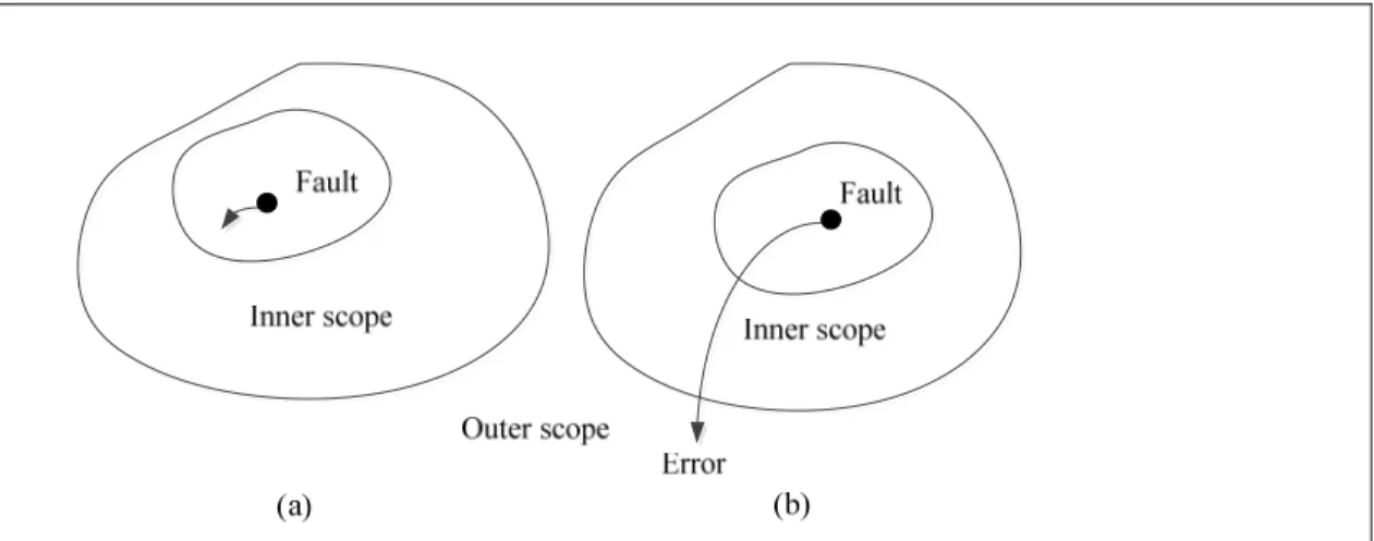
This section aims to understand the difference between faults and errors. Note that errors are the manifestation of faults. Figure 1.6 illustrates the difference between faults and errors. When a fault is not masked by the component (inner scope) and manifests itself in the outer scope, error occurs (Mukherjee 2011, p. 7).
Figure 1.6 a) Fault which is masked in inner scope b) Fault which manifests in outer scope will be called error
Adapted from Mukherjee (2011), p. 8
When an error presents itself to the user, failure is said to occur. Failure may be attributed to system malfunction leading to a deviation from the correct behaviour of the system. Errors are classified as either permanent or transient: permanent faults cause permanent errors, while transient faults cause transient or soft errors (Mukherjee 2011, p. 8). In this thesis, soft
faults or soft errors are our concern. The following section explores the way in which circuits could be verified by fault injection.
1.3 Digital circuit verification by fault injection
For modern digital circuit designs, one way to verify its behaviour is using a high-level language like VHDL. The design of the circuit should be evaluated before an actual implementation. This evaluation is based on a number of criteria such as area, power of consumption etc. By evaluating the design at a high-level of abstraction in presence of faults, the design could be modified before its actual implementation. This ability allows a desired design to be achieved after the actual implementation process. A fault injection tool could provide such ability. Note that there are two categories of faults: permanent and transient. During offline testing by the producer of the logic circuit, most of permanent faults of the circuits are recognized. Therefore permanent faults are the primary concern after a chip is purchased by the customer. To evaluate the performance of a non-line testable circuit, the capability to simulate the injection of a transient fault in the VHDL description of a circuit is necessary. This allows the performance of a circuit to be verified in faulty conditions before its actual implementation (Seward and Lala 2003).
Fault injection could be done at a low-level or a high-level of abstraction. Fault injection tools include those for fault simulation and fault emulation. Fault simulation tools are used for evaluating radiation effects and fault tolerance by applying analytical methods; however, fault emulation tools apply hardware methods. By using fault simulation and emulation tools, traditional radiation hardness assurance (RHA) techniques are improved. These steps ensure that circuit designs meet desired goals after implementation. By applying fault simulation and emulation tools, the test of the circuit design on the benchtop is allowed while ensuring that time and financial limitations for accelerated radiation testing are economized (Quinn, Black et al. 2013). In the following sections, different models used for fault injection are described and fault injection techniques are explained.
1.3.1 Fault models
Models emulate a physical reality using mathematical abstraction. For injecting faults in models of the digital circuit, fault models are defined. Two different fault models, Stuck-at and Bit-flip, are explored in this section (Borecky, Kohlik et al. 2011).
1.3.1.1 Stuck-at (s-a) fault model
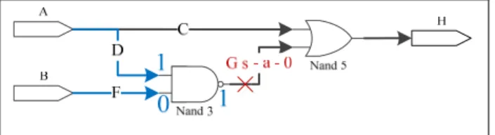
Stuck-at fault model is an abstract fault model. It models a functional fault. When stuck-at 1 model is applied a logic 0, a logical error is produced - this means the logic 0 becomes logic 1 after applying stuck-at 1 to a logic 0. The physical equivalence for this fault model are short and open connections (Patel 2005). In figure 1.7, the fault s-a-0 is activated on line G. As illustrated, this fault changes the logic value 1 to 0 on line G.
Figure 1.7 The fault s-a-0 is activated on line G when logic value 0 is applied on line G Adapted from Patel (2005)
In this thesis, single stuck-at fault model is used. In (Grosso, Guzman-Miranda et al. 2013), the authors establish a correlation between the effects of SEU and the Stuck-At (SA) faults model. According to their results, if injecting SA0 and SA1 at a specific location in a digital circuit doesn’t produce a faulty output, SEUs won’t produce error when they occur at the same location for a large majority of cases affecting the digital circuit it is a good model. However, simulation reveals that, by applying stuck-at fault model, sometimes fault injection simulator generates the same output obtained when no fault is injected. For example, when the value of a net in a circuit is 0, injecting a stuck-at 0 on that net does not have any observable effect on the circuit primary outputs.
1.3.1.2 Bit flip fault model
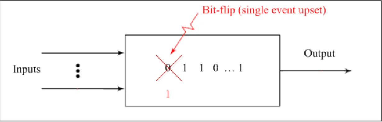
Bit flip fault model represents a modification in the state of memory. This change is caused by an SEU. As illustrated in figure 1.8, a bit flip fault changes the value of the bit memory from “0” to “1” (Borecky, Kohlik et al. 2011).
Figure 1.8 The bit flip fault injected into memory Adapted from Borecky, Kohlik et al. (2011)
It appears plausible that the bit flip fault injection model may be more efficient for this thesis. By applying bit flip fault injection, the state of the bit is always modified and there is greater correlation between bit flip fault model and SEU occurrences than between stuck-at fault model and SEU occurrences. Applying the bit flip fault model on the experimental results presented in this thesis offers the scope of future work.
1.3.2 Fault injection techniques
Fault injection is a validation technique of the dependability of fault tolerant systems, executed by observing the behaviour of the system in the presence of faults which are induced or injected into the system. There are several techniques to inject faults into a system model. They are classified into three main categories and are explained in the following sections.
1.3.2.1 Hardware-based injection techniques
In the hardware-based fault injection technique, a system is tested by specially designed test hardware for the injection of faults into the target system and examining its effects. These kinds of faults are injected at the pin level of the Integrated Circuit (IC). For transistors, stuck-at, bridging, or transient faults are injected and circuit operation thereafter allows their effects to be examined.
Hardware fault injections are applied to the actual circuit after fabrication. By using some sort of interference which could produce and inject fault into the circuit, the behaviour of the circuit in the presence of fault is examined. This injection technique consumes time to prepare and thereafter test the circuit of interest. Testing the circuit by this method is faster than simulation, although the motivation behind testing a circuit before the delivery to the costumer is pretty obvious (Alfredo Benso 2003).
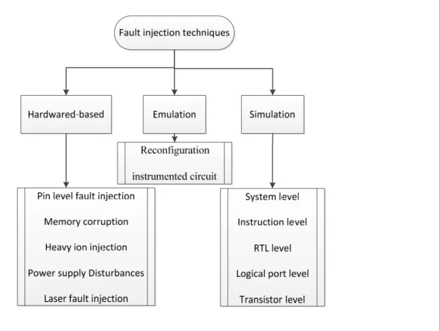
In figure 1.9, some examples of this technique are presented (Ziade, Ayoubi et al. 2004). In the following sections, other techniques for fault injection are defined.
1.3.2.2 Emulation-based injection techniques
FPGAs could be used to emulate the circuit behaviour at hardware speed and are therefore used to speed up the process of fault injection. The principle behind this technique is to execute tasks accomplished by simulation-based fault injection techniques using an FPGA. The problem with using such techniques is about retaining the flexibility of a simulation-based approach. With more tasks transferred from the computer to the FPGA, the controllability and observability of the process under test decreases. These approaches are faster than simulation-based techniques, but communication bottlenecks while data is transferring between the computer and the FPGA pose the main problem. In fact in these approaches, a major part of the task is accomplished using hardware, while the rest is
executed in the computer (Valderas, Garcia et al. 2007). There are two categories for fault injection by using FPGA emulation approaches - by using instrumented circuit technique, or partial reconfiguration technique. In partial reconfiguration methods, by reconfiguring the proper FPGA cell, a flip flop value is modified. It is usually done by resetting the flip flop (Antoni, Leveugle et al. 2002). In the instrumented circuit method, all circuit flip-flops are replaced by a more complex structure. In this way, fault injection may be controllable externally. The flip-flop substitution includes a fault mask and an injection enable signal. The fault mask allows the fault localisation to be selected, while the injection enable signal allows controlling the fault time instant (Lima, Rezgui et al. 2001).
SEU Controller is a tool created by Xilinx that can be included in any design using the Virtex-5 FPGA family or higher. This tool allows us to detect and correct SEU, but also used to emulate SEUs within the Virtex-5 device. By applying SEU controller, errors injection in a controlled and predictable way into the configuration memory can be done (Chapman 2010).
1.3.2.3 Simulation-based injection techniques
Simulation-based fault injection is when faults are injected in models of the system using a fault simulator. Different modeling languages can be used like VHDL, SystemC, etc. In this way, the system dependability may be evaluated when only the model of the system is developed. By using different description languages, this approach could address different levels of abstraction (Ziade, Ayoubi et al. 2004). Figure 1.9 presents these different levels.
Figure 1.9 Classification of fault injection techniques Adapted from Ziade, Ayoubi et al. (2004)
Hardware simulation is used in this thesis and occurs at a low-level of abstraction of the circuit. Faults are injected into the gate level description of the circuits. Thereafter, the system is simulated and the response of the circuit to that particular fault is evaluated.
1.4 Developing fault behavioural model
In this section, the two most popular fault injection techniques at a high-level of abstraction are discussed, and the way in which they are applied to the system is explained.
Saboteur: A saboteur is a VHDL component added to the original model, the goal of which
is to change the value of one or more signals which is simulating the occurrence of a fault. To ensure normal operation of the system, this component may be made inactive. Ports of the
components in the model are affected by the saboteur. Therefore, for applying a saboteur, structural descriptions are needed. (Baraza, Gracia et al. 2008).
Mutant: A mutant is a component which replaces another component. While it is inactive, it
behaves like the original component in existence of faults. Three ways may be used for developing mutation (Baraza, Gracia et al. 2008):
• in structural model descriptions, saboteur is added;
• structural descriptions are modified and sub-components are replaced. For example a NOR gate could be replaced by a NAND gate;
• in behavioral descriptions, syntactical structures are modified.
By using both techniques, fault behaviour models may be developed and used to find out how systems behave in presence of faults at high-level of abstraction. In this way, the reliability of the circuit could be studied early during the design flow itself. Our main concern in the work presented here is to capture the faulty behaviour of a component, so as to enable a realistic injection of fault. Neural networks are a viable solution for that. A neural network may be used to learn this faulty behaviour. In the following section, neural network and its advantages for capturing the faults in a system are studied.
1.5 Neural network and fault
The neural network has been used for fault diagnosing and fault clustering in digital and analog circuits before. The following describes some areas of using neural network approach for digital or analog system in presence of faults.
In (Al-Jumah and Arslan 1998), feed forward artificial neural networks are used for the diagnosis of multiple stuck-at faults in digital circuits. In their technique, a fault truth table is developed by injecting single random stuck-at fault in the circuit, and the result data is used to train the neural network. The results show that an efficient and flexible neural network is obtained, which is capable of diagnosing multiple stuck-at faults.
In (Whei-Min, Chin-Der et al. 2001), a new approach to detect fault types in a transmission line (which is an analog circuit component) is presented. A Neural network is used to detect various patterns of correspondent voltages and currents. In the paper, radial basis function (RBF) neural network is compared with back propagation neural network, and results show that RBF can provide the faster and more accurate model.
In (Lifen, He et al. 2010), a new fault detection method for analog circuits is presented. In their work, the output signal of the circuit under test is studied and the kurtoses and entropies of the signals are determined. These characteristics are used to measure the signal’s higher order statistics. The kurtoses and entropies are used as inputs of neural network in training phase to develop fault classifier neural network model. The proposed method works with high accuracy for nonlinear analog circuits. This method can classify both soft and hard faults.
Previous studies show that the neural network approach is appropriate to be applied for fault clustering and fault diagnosis in digital and analog circuits. Neural networks are able to learn non-linear relations between data. After learning, Artificial Neural Network (ANN) structure could estimate a function for mapping input-output pairs. Furthermore, the trained ANN has the ability of generalization - which means that it could produce almost the desired outputs for inputs which are not participating in the training process.
For developing fault behaviour model of the digital circuit, it needs to have a component which is able to generate outputs of a circuit. The mentioned ability of ANN seems to be useful to develop that component. The faulty behavior of the circuit could be trained by ANN, following which the trained ANN may be used to generate faulty output of circuits. In the course of this thesis, the possibility of applying the neural network to develop the faulty behaviour model of digital circuits in presence of faults or no is explored. The next chapter will explore neural networks, and present the information needed to develop one.
1.6 Conclusion
In this section, cosmic rays are introduced, and explain how they cause faults in digital circuits. Afterwards, fault models are discussed and fault injection techniques are explained. Finally, neural network and its advantage with regard to fault diagnosis and fault clustering are discussed. As neural networks are used for fault recognition in digital circuit, it promises to be useful for developing fault behavioral model as well. In this thesis, a new way of developing fault behavioural model at a high-level of abstraction by using the neural network approach is explored. In the next chapter, neural networks are studied, and the benefits regarding the way in which neural network fault behavioral model maybe developed is explained.
CHAPITRE 2
NEURAL NETWORKS AND THEIR APPLICATIONS IN FAULT MODELS
In this chapter, neural networks are explained. First, the neuron is described and then neural network architectures are presented. Multilayer perceptron (MLP), which is one of the most common classes of neural network, is also explained in detail. To use neural networks efficiently, there are some tips that should be considered. Section 2.5 illustrates how to use the MLP neural network in practice. In short, this chapter presents how to develop a neural network for a specific problem.
2.1 A brief introduction to artificial neural networks
A common problem in engineering fields is to estimate a function, which can map input-output pairs. This is referred to as supervised learning by the neural network (Cerny and Proximity 2001). The training set is composed of pairs of independent (input) and dependent (output) variables. The neural network represents the map function between input vectors ( ) and output vectors ( ) according to the following equation:
= ( ) ( 2.1)
Where is a vector for inputs and is a vector for outputs of the system under investigation.
Neural network models have two different categories: supervised neural networks (such as the multilayer perceptron), or unsupervised neural networks (such as kohonen feature maps). For supervised neural networks, training and testing data are used to build the model, and the data includes input patterns with the corresponding output values. For unsupervised neural networks, the network decides what output values are best for the current input pattern, and there is no predetermined output value for any input pattern (Cerny and Proximity 2001).
In fact, a neural network is a huge parallel and distributed processor, which has the capability of storing information. It is similar to the human brain in three aspects:
• knowledge of neural network is acquired by learning process;
• synaptic weights, which are inter-neuron connection strengths, are responsible for storing knowledge;
• the network has the ability to generalize.
The process of learning is achieved through what is referred to as a learning algorithm. Changing synaptic weights to achieve a desired design goal is the objective of the algorithm. The trained network has the ability of generalization, which means that it can produce almost all the desired outputs for the inputs patterns that are not participating in the training process.
In the following, neural network characteristics which are relevant to this thesis are specified:
Learning algorithm: one of the more popular classes of learning algorithm is supervised
learning. The network is fed with input samples, and weights of the network change so as to minimize the difference between the value observed at the output of the network and the desired output value. Learning is stopped when there are no more significant changes in the value of the weights;
Ability of nonlinear mapping: a neuron is a nonlinear element is a nonlinear activation
function in a neuron which produces an output from the weighted input. Therefore, a neural network (which is composed of neurons) is a nonlinear mapping model. In the next section, a neuron and its activation function are explained in details;
Ability of adaption: a neural network is trained for a specific task in a specific environment
(input-outputs pairs). However, it should be able to deal with a small change in the environment, and this is referred to as the ability of adaption of the neural network.
The most common neural network for supervised learning is the multilayer perceptron (MLP) which was established in 1986 (Jain, Mao et al. 1996). As illustrated in figure 2.1, the MLP is composed of feed-forward connections with adjustable weights. Training of the MLP refers
to the estimation of the best set of weights while the error between the network output and the desired output is minimized (Farhat 2003).
X1 X2 X3 Y Z1 Z2 Input layer Hidden
layer Outputlayer
w1 w2
w3
v1
v2
Figure 2.1 A small example of an MLP neural network with one hidden layer Adapted from Fausett (2006)
In figure 2.1, neuron sends its output to neurons , with respective connection weights and . The received signals by and are different according to the different scales which come from the different weights and on their links. Note that this is a very simple neural network with a hidden layer and a nonlinear activation function (Fausett 2006).
2.2 The neuron
A neural network is an information processing system. It shares common characteristics with biological neural networks. In fact, it is a mathematical model of human cognition or neural biology. Such a model is based on the following assumptions:
• an artificial neuron (perceptron), which is shown in figure 2.2, is a very simple element where information processing occurs;
X1 X2 X3 Y w1 w2 w3
Figure 2.2 A simple element which is called artificial neuron or perceptron. , , and are neurons or perceptrons; The weights on the links to neuron from neurons , and
are , and Redrawn from Fausett (2006)
• there is a connection link between any two neurons for passing signal;
• for each link, a weight is associated and this weight is multiplied to the signal transmitted;
• each neuron determines its output by applying an activation function to its input which will be discussed in details.
Each neuron behaves as a function; it transmits an input signal to an output signal ( ). The function ( ) could be assumed in different forms. It could model basic activation functions such as the sigmoid, the threshold or the radial basis function. In figure 2.3, the sigmoid activation function is illustrated. In the rest of this chapter, activation functions are further explained.
Figure 2.3 The sigmoid activation function
Each neuron has an internal state which is a response of the activation function to the input of the neuron. This internal state is called the activity level of the neuron, or the neuron’s activation. The internal state of each neuron is broadcast as a signal to all the connected neurons via connection links.
In figure 2.2, consider the neuron that is connected to three neurons , and . The activation of these three neurons are , and . The weights on the links to neuron from neurons , and are , and . Input of neuron , , is the sum of the signals from neurons , and , that is:
Activation of neuron , = ( ), is calculated with a function of its input signals. As explained before, there are several activation functions and the logistic sigmoid (2.3) is one of them:
( ) = 1
1 + (− )
(2.3)
In the following section, neural network architectures are explained.
2.3 Neural network architectures
Neuron arrangement and the way in which they are connected together have a strong effect on the learning algorithm used to train the network. Neural network architectures are classified into three main categories as illustrated in figure 2.4 (Haykin 2001):
• single layer feed forward;
• multi-Layer Perceptron feed forward (MLP); • recurrent network.
(a) (b) (c)
Figure 2.4 The different architectures for neural network: a) single layer feed forward, b) multi-layer perceptron feed forward, c) recurrent network
Adapted from Haykin (2001)
In this thesis the MLP network architecture is used, which is also the most well-known and widely used topology. They are able to represent non-linear mapping between inputs and
outputs, and are universal approximations (Yu 2000, Cerny and Proximity 2001). Feed forward neural networks seem well suited for the purpose of the work here; as a black box, it facilitates the development of the fault behavior model of the circuit by considering only the inputs and the outputs of the circuit without any information of the circuit details. In addition, generalization ability of the neural network helps us to perform sampling by considering only part of the data, enabling the neural network model to map the remaining after training. In the following section, multi-layer neural networks trained by the back propagation algorithm are explained in detail.
2.4 Multi-layer perceptron (MLP) networks
Consider n as the number of input neurons and m as the number of output neurons of a neural network. Let be a dimensional vector which contains all inputs of the neural network and y be an m dimensional vector which contains all outputs of the neural network. In addition, let be a vector representing all weights used for internal connections between the neurons. The structure of a neural network is defined according to the choice of values for all weights in the vector . This means that how the output of the neural network ( ) is computed from the input vector is determined by choosing values for the elements of the vector . The following equation (2.4) mathematically represents a neural network model (Zhang, Gupta et al. 2003).
= ( , ) (2.4)
The learning by the neural network happens using the weights of the connection links. Therefore to solve more complicated problems, more links should be added. To increase the number of links, there are two options (Marsland 2011):
Add backward connections: using this technique, the output of the neural network is
connected to the input of the neural network, and recurrent neural networks are developed as shown in figure 2.4 c);
Add more neurons: by adding more layers of neurons between the input and the output
layers, multilayer neural network architecture is developed: figure 2.4 b).
A neural network can solve non-linear problems by including a hidden layer in its architecture. Neural networks with hidden layer have the ability to solve many more problems than can be done using a simple neural network without hidden layers. Such an ability may be attributed to the non-linear relation between its input and output neurons (Fausett 2006).
As illustrated in figure 2.5, neurons in MLP neural networks are grouped into layers. The first layer is the input layer and the last layer is the output layer. All the middle layers are called hidden layers.
Figure 2.5 The multilayer perceptron neural network structure Adapted from Zhang, Gupta et al. (2003)
Suppose is the number of neuron in the th layer, = 1, 2, … , . is the weight of connection between th neuron in the − 1th layer and th neuron of the th layer. is the th input of the neural network and is the output of the th neuron of the th layer. represents the bias for the th neuron of the th layer. In equation (2.5), vector of the neural
network includes all while = 0, 1, … , , = 1, 2, … , , = 2, 3, … , (Zhang, Gupta et al. 2003).
= , … , (2.5)
Each neuron has a threshold value which determines when the neuron state will be changed. When the input of a neuron is more than the threshold , the neuron fires : this means that the state of the neuron is changed. When the neuron input is less than the threshold , nothing happens and the neuron remains in its current state. Threshold should be adjustable in order to have a changeable value for firing each neuron. For enabling this capability, we add an extra input weight to each neuron with fixed inputs. This weight is updated during the learning phase, similar to other weights, in order to adjust if the neuron fires or not. This input node is called bias. The bias node has weight connecting to th neuron (Marsland 2011).
2.4.1 Preliminaries definitions for MLP learning algorithm explanation
Some preliminary definitions are now explained which will be used to explain the MLP learning algorithm:
Inputs : it is the input vector with elements , where is from 1 to input dimension (m);
Weights : it is the weight value of the connection signal between node and ;
Outputs : it is the output vector with elements , where is from 1 to output dimension (n);
Target : it is the target vector with elements , where is from 1 to output dimension (n). We will use this vector during supervised training. It contains the correct outputs that a neural network uses during training phase;
Activation function : it is a mathematical function which works like the threshold function
described earlier. It expresses the firing of a neuron as a reply to weighted inputs;
The learning rate : it describes how much the weights are changing in order to decrease
errors between current outputs and target outputs. It lies in the range specified by 0.1 < < 0.4 (Marsland 2011) and depends on the amount of error we expect from the input.
2.4.1 MLP learning algorithm description
The following describes the steps of Multi-Layer Perceptron training algorithm. This is also called back propagation learning (Marsland 2011). In figure 2.6, the steps of this algorithm are illustrated.
The steps of the MLP algorithm are now explained in greater detail.
In the Initialisation step, all weights are initialized to small random values (positive and negative).
In the Training step there are two phases:
Forward phase: calculate the activation of each neuron of the hidden layer by the
following formula ( is a positive parameter). First, ℎ (which is the addition of all weighted inputs of neuron of the hidden layer) is calculated by formula (2.6), and then by using it in formula (2.7) which gives activation function ( ), the output of neuron ( ℎ ) is calculated;
Go forward through network such that output layer has the following activation function:
Backwards phase: calculate the error at the output layer with the formula (2.10):
Calculate error in hidden layer with following formula:
ℎ = (2.6) = ℎ = 1 1 + exp(− ℎ ) (2.7) ℎ = (2.8) = (ℎ ) = 1 1 + exp(− ℎ ) (2.9) = (t − y )y (1 − y ) (2.10)
Weights of output layer is updated using the following: ( is the weight of the first hidden layer)
← w + ηδ a (2.12)
Weight of hidden layer is updated as following: ( is the weight of the first hidden layer)
← v + ηδ x (2.13)
In the next section, activation function in neuron element is explained in details.
2.4.2 Neuronal activation functions
The functions in the hidden layer are not identical as the ones in the output layer. There are a lot of different activation functions to produce an output from the weighed input. The activation function is selected according to the task of the neuron. In figure 2.7, the most common activation functions are illustrated.
Hard limit activation function: if the neuron input reaches some threshold, this function
sets the neuron output to 1, and otherwise to 0.
The symmetrical hard limit activation function: if the neuron input reaches pre-specified
threshold, this function sets the neuron output to 1, and otherwise to -1.
The linear activation function: this function multiplies neuron input signal by a constant
scale and after adding bias value to it, the signal is transmitted to the neuron output.
The saturated linear activation function: this function works the same way as the linear
activation function while the neuron input is between [-1, 1]; the neuron output is set to 1 when the neuron input is more than 1, and the neuron output is set to -1 when the neuron input is less than -1.
The log sigmoid: by using this function, while input varies between −∞ to ∞, the neuron output is between [0, 1]. This is a differentiable function and is useful for back propagation training algorithm.
The tan-sigmoid activation function: by using this function, while input varies between
Figure 2.7 Commonly used activation functions for a neuron, where O/P denotes the output of the neuron and I/P denotes the input
Adapted from Farhat (2003)
Generally, the linear functions are suitable for the neuron in the output layer while the sigmoid functions are suitable for the neuron in the hidden layer.
2.5 Multi-layer perceptron in practice
In this section, the process to determine the parameters to develop the network is explained. According to difference in number for these parameters, the neural network will be adjusted to find solutions for different kinds of problems.
2.5.1 Data preparation
With pre-processing on input and target datasets before training, most of the neural network and machine-learning algorithms work with greater precision. For example, if the activation function for output is the sigmoid function, the target values should be between 0 and 1. Regardless of which activation function used, it is normal to scale target values between 0 and 1 to ensure weights do not get too large. Also, the input dataset may be scaled to avoid increasing the number of required weights. The most common method for MLP is to scale each data dimension to have a zero mean and a unit variance. Scaling data while maximum is 1 and minimum is -1 will result in a zero mean value and unit variance value. This scaling is called normalization or standardization. Though normalization for MLP is not necessary and only ensures better results, for some neural network it is necessary since without normalization, they cannot learn the relation between input and output sets (Marsland 2011).
2.5.2 Size of training data
For a neural network with one hidden layer, the number of weights is ( + 1) × + ( + 1) × , where is the number of nodes in the input layer, is the number of nodes in the hidden layer and is the number of nodes in the output layer. The extra +1s are for bias nodes which have adjustable weights. The weights of connection links between neurons are set during the training phase. Back propagation algorithm is responsible for setting the values of weights and these values are determined from the error calculated from data during the training phase. It is obvious that with more training data, learning is better although the time of training phase is consequently more. Unfortunately, there is no way to determine the minimum amount of training data, and it depends on the problem. Based on rule of thumb, the amount of training data should be at least ten times the number of connection links. This
is a large number and training the neural network is a computationally expensive operation (Marsland 2011).
2.5.3 Number of hidden layers
There are two more considerations for neural networks: the number of hidden layers, and the number of nodes in them. Later, it is explained why two hidden layers is the maximum amount that an MLP neural network needs. Note that there is no theoretical guide for selecting the number of nodes in hidden layers and they could be specified practically. In practice, by testing the neural network with different number of nodes in the hidden layers, the best number is found. For the back propagation algorithm, it is possible to have any number of hidden layers, but as mentioned before, normally, two hidden layers is the maximum which is needed. The reason for this is that approximate the mapping of any smooth functional by a linear combination of sigmoidal activation functions is possible. Therefore, any decision boundary (besides linear ones) may be approximated by a neural network. Here, the lines which classify different data are called decision boundary (Marsland 2011).
2.5.4 Generalization and over-fitting
Generalization is the whole purpose of using neural networks to compute the output for all possible input patterns based on training samples. We have to be sure that the neural network has been trained enough to be able generalize well. There is also the danger of over fitting. If training is performed for too long, data will be over fitted, which means that besides the actual function, noise is also learnt. When over fitting happens the trained neural network is too complicated and cannot generalize. Figure 2.8 shows two data sets. White ones are training data and red ones are evaluation data. The lines are the estimation of training data set which comes from the functions trained by the neural network. The right figure shows over fitting results. The estimated line passes all training data (white ones). This line is too complicated and cannot predict evaluation data (red ones). In contrast, the left figure shows the ability of generalization. The line doesn’t pass all the training data (white ones), but is an
estimation of training data. This neural network didn’t train noise and has the ability to predict evaluation data (red ones).
Solution for over fitting problem has two parts. First, the training has to be stopped before over fitting occurs. Second, the neural network has to be tested (Marsland 2011). In the next section, this is explained in details.
Figure 2.8 There are two data sets. White ones are training data and red ones are evaluation data. The lines are the estimation of training data set which comes from the functions which are trained by the neural network. The left neural network has the ability of generalization
but the right neural network exhibits over fitting. Adapted from Johnson ( 2013)
2.5.5 Training, testing, and validation
The error of a trained neural network is calculated by the sum-of-squares error between the computed output and the targeted output. The test should be done with the data, which is not used for training in order to see how well the trained neural network generalizes and if over-fitting has occurred. Therefore, we have to keep a reserve dataset for testing that has not been used for training.
During training, it is necessary how well the neural network works, and to decide if it is a good time to stop or not. For this purpose, if we use the training data set, over-fitting cannot