Design for Optimized Multi-Lateral Multi-Commodity Markets

Texte intégral

(1)2003s-36. Design for Optimized Multi-Lateral MultiCommodity Markets Benoît Bourbeau, Teodor Grabriel Crainic, Michel Gendreau, Jacques Robert. Série Scientifique Scientific Series. Montréal Juin 2003. © 2003 Benoît Bourbeau, Teodor Grabriel Crainic, Michel Gendreau, Jacques Robert. Tous droits réservés. All rights reserved. Reproduction partielle permise avec citation du document source, incluant la notice ©. Short sections may be quoted without explicit permission, if full credit, including © notice, is given to the source..

(2) CIRANO Le CIRANO est un organisme sans but lucratif constitué en vertu de la Loi des compagnies du Québec. Le financement de son infrastructure et de ses activités de recherche provient des cotisations de ses organisationsmembres, d’une subvention d’infrastructure du ministère de la Recherche, de la Science et de la Technologie, de même que des subventions et mandats obtenus par ses équipes de recherche. CIRANO is a private non-profit organization incorporated under the Québec Companies Act. Its infrastructure and research activities are funded through fees paid by member organizations, an infrastructure grant from the Ministère de la Recherche, de la Science et de la Technologie, and grants and research mandates obtained by its research teams. Les organisations-partenaires / The Partner Organizations PARTENAIRE MAJEUR . Ministère du développement économique et régional [MDER] PARTENAIRES . Alcan inc. . Axa Canada . Banque du Canada . Banque Laurentienne du Canada . Banque Nationale du Canada . Banque Royale du Canada . Bell Canada . Bombardier . Bourse de Montréal . Développement des ressources humaines Canada [DRHC] . Fédération des caisses Desjardins du Québec . Gaz Métropolitain . Hydro-Québec . Industrie Canada . Ministère des Finances [MF] . Pratt & Whitney Canada Inc. . Raymond Chabot Grant Thornton . Ville de Montréal . École Polytechnique de Montréal . HEC Montréal . Université Concordia . Université de Montréal . Université du Québec à Montréal . Université Laval . Université McGill ASSOCIÉ AU : . Institut de Finance Mathématique de Montréal (IFM2) . Laboratoires universitaires Bell Canada . Réseau de calcul et de modélisation mathématique [RCM2] . Réseau de centres d’excellence MITACS (Les mathématiques des technologies de l’information et des systèmes complexes) Les cahiers de la série scientifique (CS) visent à rendre accessibles des résultats de recherche effectuée au CIRANO afin de susciter échanges et commentaires. Ces cahiers sont écrits dans le style des publications scientifiques. Les idées et les opinions émises sont sous l’unique responsabilité des auteurs et ne représentent pas nécessairement les positions du CIRANO ou de ses partenaires. This paper presents research carried out at CIRANO and aims at encouraging discussion and comment. The observations and viewpoints expressed are the sole responsibility of the authors. They do not necessarily represent positions of CIRANO or its partners.. ISSN 1198-8177.

(3) Design for Optimized Multi-Lateral MultiCommodity Markets Benoît Bourbeau*, Teodor Gabriel Crainic†, Michel Gendreau‡, Jacques Robert§. Résumé / Abstract Nous présentons un concept de marché optimisé, centralisé, multilatéral et périodique pour l’acquisition de produits qui traite explicitement les trois aspects suivants: (i) des coûts de transport importants des vendeurs vers les acheteurs; (ii) des produits non homogènes en valeur et qualité; des complémentarités entre les divers produits qui doivent donc être négociés simultanément. Le modèle permet aux vendeurs d’offrir leurs produits groupés en lots et aux acheteurs de quantifier explicitement leur évaluation des lots mis sur le marché par chaque vendeur. Le modèle ne suppose pas que les produits doivent être expédiés par un centre avant d’être livrés. Nous proposons également un mécanisme de tâtonnement à rondes multiples qui approxime le comportement du marché direct optimisé et qui permet de mettre ce dernier en oeuvre. Le processus de tâtonnement permet aux vendeurs et aux acheteurs de modifier leurs mises initiales, incluant les contraintes technologiques. Les concepts proposés sont particulièrement adaptés aux industries reliées aux matières premières. Nous présentons les modèles et algorithmes requis à la mise en oeuvre du marché multi-latéral optimisé, nous décrivons le fonctionnement du processus de tâtonnement, et nous discutons les applications et perspectives reliées à ces mécanismes de marché. Mots clés : Design de marché, marché multi-latéraux optimisés, processus de tâtonnement.. In this paper, we propose a design for an an economically efficient, optimized, centralized, multi-lateral, periodic commodity market that addresses explicitly three issues: (i) substantial transportation costs between sellers and buyers; (ii) non homogeneous, in quality and nature, commodities; (iii) complementary commodities that have to be traded simultaneously. The model allows sellers to offer their commodities in lots and buyers to explicitly quantify the differences in quality of the goods produced by each individual seller. The model does not presume that products must be shipped through a market hub. We also propose a multi-round *. CIRANO, email: [email protected]. Département management et technologie, Université du Québec à Montréal and CIRANO and Centre de recherche sur les transports, Université de Montréal/École Polytechnique/HEC Montréal, email: [email protected]. ‡ Département d’informatique et recherche opérationnelle, Université de Montréal and CIRANO and Centre de recherche sur les transports, Université de Montréal/École Polytechnique/HEC Montréal, email: [email protected]. § Département des Technologies de l’information, HEC Montréal and CIRANO, email: [email protected]. †.

(4) auction that enables the implementation of the direct optimized market and approximates the behaviour of the “ideal” direct optimized mechanism. The process allows buyers and sellers to modify their initial bids, including the technological constraints. The proposed market designs are particularly relevant for industries related to natural resources. We present the models and algorithms required to implement the optimized market mechanisms, describe the operations of the multi-round auction, and discuss applications and perspectives. Keywords: Market design, optimized multi-lateral multi-commodity markets, multi-round auctions..

(5) 1. Introduction. Until very recently markets were not designed, they just existed. Markets emerged out of uncoordinated private initiatives and, in most cases, there are still no explicit rules that determine how equilibrium prices are discovered and set. In most markets, prices are posted by sellers or negotiated bilaterally according to informal rules. Recently, however, the design of market rules has emerged as a very important issue due to three main factors: (i) The creation by government agencies, private firms or industrial associations of a number of markets to privatize public assets, restructure deregulated industries, or enhance inter-firm relations; (ii) A renewed focus on strategic analysis and game theory that together with the emergence of experimental economics contributed to the establishment of market design as a serious research field in economics; (iii) And, most importantly, the explosive development of electronic business, e-business tools that can embed the most complex market rules and facilitate their deployment. This paper examines the problem of designing optimized or smart markets. An optimized or smart market is an advanced exchange mechanism. It is a competitive environment where buyers and sellers interact and is designed to solve possibly complex allocation problems. According to Miller (1996), “the distinctive characteristic of a smart market is that it can manage complex contingencies embedded within orders in a consistent and effective manner.” A smart market would generally require an optimization device in order to clear the market while taking into account the implicit or explicit constraints and contingencies submitted to the market marker. There are typically two types of constraints: complex order requirements as submitted by the participants and feasibility requirements as some orders may not be jointly fulfilled. A number of smart market mechanisms have been proposed for pricing the Internet (MacKie-Mason and Varian 1995; MacKie-Mason 1997) and for allocating accesses to a railway network (Brewer and Plott 1996), airport take-off and landing slots (Rassenti, Smith, and Bulfin 1982; Grether, Isaac, and Plott 1989), and pollution permits (Marron and Bartels 1996), as well as for the scheduling of the Space station resources (Ledyard, Porter, and Rangel 1994), the distribution of electricity within a grid (Rothkopf, Kahn, Teisberg, Eto, and Nataf 1990), and the matching of supply and demand in financial markets (Fan, Stallaert, and Whinston 1999). A number of authors have also addressed issues related to the optimization formulations of market clearance mechanisms, in particular in combinatorial auctions (e.g., Rothkopf, Pekeˇc, and Harstad 1998; Sandholm 1999; De Vries and Vohra 2001; Kalagnanam, Davenport, and Le 2001; DeMartini, Kwasnica, Ledyard, and Porter 1999) where participants may submit “all-or-nothing” package bids. Yet, relatively few actual implementations of smart markets have been observed up to now. Furthermore, very limited efforts have been dedicated to the design of the whole market mechanism (Abrache, Crainic, and Gendreau 2001). With a growing interest on the use of combinatorial auctions for spectrum rights, the trend seems to be changing, however, and a consensus appears to emerge that optimized markets can be profitably used in complex environments where global efficiency is highly desirable. Therefore, the general objective of this paper is to contribute to the development of the basic methodology leading to the design 1.

(6) and practical implementations of optimized markets. A market design must specify clear negotiation rules. These include two main elements. First, one must specify an explicit mathematical representation for the market-clearing procedure that identifies, given the submitted bids, the market allocation, who produces what and sells to whom and in what quantities, and prices, who pays what to whom. Formally, under certain conditions, a market-clearing mechanism can be represented as a constrained optimization problem. The bids define the parameters of the constrained optimization problem, while the solution of the problem yields the quantity allocation (the primal) and the corresponding prices (usually based on dual information). Second, the market design must specify how negotiations will proceed. It is well known, in effect, that participants often are unwilling or unable to disclose all the pertinent but very personal and proprietary information required for an optimized market. Moreover, formal incentive mechanisms cannot be defined for many important market cases, including the multi-lateral type of market considered in this paper (Myerson and Satterthwaite 1983). Open, multi-round negotiations are therefore increasingly considered. Such multi-round auctions require significantly less a priori information and allow participants to alter their selling or buying offers in light of the market information and their own assessment of the market. At each round, the auction makes use of the optimization procedure to produce a temporary set of allocations and prices. The process continues until no one wishes to alter its bid and the bilateral exchanges then become official. In order to prevent the negotiation from lasting for ever, the rules must specify not only the stopping rule, however, but also eligibility and activity rules whose function is to give impetus to the market by prompting participants to be active and progressively commit themselfs. We focus on the design of optimized multi-lateral markets for geographically dispersed heterogeneous commodities and technological constraints. Based on well-known economic principles, we define an economically efficient optimized multi-lateral market that addresses explicitly four issues: (i) the non homogeneity in quality and nature of the commodities traded, (ii) the buyers’ qualification of the differences in quality of the goods produced by each individual seller, (iii) the existence of complementarities between commodities and the need to negotiate these simultaneously, (iv) the presence of substantial transportation costs between sellers and buyers. We strongly believe that when transportation costs are significant, they should be explicitly accounted for in the optimization of the market. How this can be achieved in practice is one of the main contributions of the paper. We present the appropriate optimization formulations and algorithms, and define an open, multi-round auction mechanism that enables the implementation of the optimized multi-lateral market and approximates its behaviour under “ideal” information conditions. We show how such a mechanism may be operationalized and present simulation results that illustrate some of the gains that can be obtained by using smart market mechanisms. Finally, we report on some of the difficulties encountered in “selling” the proposal to industrial actors. The paper is organized as follows. Section 2 presents the optimization formulation we propose to model the operations of the centralized market mechanism. We introduce the 2.

(7) main concepts and notation, present the model, and derive the market equilibrium conditions. Section 3 describes the optimization algorithms used to determine the optimal allocation and prices. Section 4 is dedicated to the presentation and analysis of the multi-round auction mechanism and the description of how negotiations are conducted. Section 5 briefly describes the Québec wood chip industry, which prompted the work presented in this paper, and presents the simulation results. Double-sided markets of the type studied in this paper are hard to analyze from a formal point of view. In particular, there is no theory describing how participants interact in such a market and classical incentive mechanisms do not apply. Therefore, Section 5 also presents a strategic analysis of the proposed market mechanism and addresses the issue of applying it, both in general and in the particular context of the wood chip market. We conclude in Section 6.. 2. Allocation Mechanisms for Optimized Multi-lateral Multi-commodity Markets. We propose a design for an optimized, centralized, multi-lateral, periodic commodity market. The market opens up periodically (once a day, once a week) and the agents in the corresponding economic sector negotiate using the centralized and optimized market. All possible multi-lateral trades are thus solved simultaneously. Commodities are classified by type or quality. Sellers may offer several commodity types separately or mixed up in lots. Buyers need to combine different grades and qualities, while technological constraints limit the quantities of each type of commodity they may acquire. Transportation costs are significant. The objective of this type of markets is to explicitly optimize both the production and transportation of resources in the industry. At the core of the market lies a market-clearing mechanism: a formal procedure that determines the “optimal” allocation - who sells what (how much) to whom and at what price - of goods given the participants and the market state. Participants are asked to communicate to the central market their production cost or demand functions (their willingness to pay), together with all relevant technical information: transportation costs, technical constraints, etc. The market then maximizes buyers’ surplus minus the production and transportation costs subject to all technological constraints. The output of the allocation mechanism are prices and quantities that equilibrate supply and demand, and that are the solution (dual and primal) of an optimization (maximization) formulation. This approach applies for a market with a simple structure as well as for more complex markets. To fix ideas, consider first a simple market where a unique homogeneous commodity is traded between one buyer and one seller. Assume no transportation costs are involved. Assuming the buyer and seller have quasi-linear utilities in money, their preferences are given by U(q) − S and S − C(q), respectively, where q is the quantity sold by the seller against a payment of S. In such a market, total profit is maximized and efficiency is obtained by solving the optimization problem maxq {U (q) − C(q)}. 3.

(8) At the optimum allocation, q∗ , the marginal willingness to pay, U 0 (q ∗ ), equals the marginal production cost, C 0 (q ∗ ). Following the Marshallian partial equilibrium tradition, this is no different from equalizing supply and demand, where the demand and supply functions correspond to the marginal utility and cost curves, respectively. The equilibrium price is given by p∗ = U 0 (q ∗ ) = C 0 (q ∗ ). Transportation costs may be considered by explicitly introducing them into the optimization problem. For a constant transportation unit cost t, one needs to solve maxq {U(q) − C(q) − tq}. The buyer then pays p∗ = U 0 (q ∗ ) = C 0 (q ∗ ) + t per unit purchased, the seller receives p∗ − t = C 0 (q ∗ ), and the carrier receives t per unit. This approach may be generalized to more complex environments as described in the following subsection.. 2.1. The Optimized Allocation Mechanism. The objective is to formulate a model to represent the products on sale in the market, the preferences of buyers and sellers regarding these products, the technological constraints buyers face, the transportation costs associated to delivering the products to the buyers. The goal is to maximize the buyers’ surplus, to obtain a so-called efficient market. The model is to be solved by mathematical programming techniques: the primal solution corresponds to the optimal quantities bought, while the dual yields the optimal prices. Let K be the set of products. The definition of a product is domain specific. Generally speaking, however, a product is a generic classification reference, such as a quality of ore, a wood species, a type of grain, etc. It is a commodity differentiated by type and quality. Even though the number of products in a market may be limited, products can be variously combined in different lots that sellers and buyers may trade. To simplify the presentation (but with no loss of generality), a lot l ∈ L is sold by one and only one seller. It is attached to a specific location and has its own idiosyncratic quality. Since a producer may sell more than one lot, the number of lots may exceed the number of producers. More importantly, a lot has its own composition of various products. For example, a stack of wood chips may contains 60% of high density fiber, 35% of low density fiber, and 5% of grey pine. Before refinement, a stack of ore or a barrel of petroleum may contain different types of ores or oils and, in practice, it may be sold before the different types P of oils or ores are separated. Let k bl denote the proportion of product k ∈ K in lot l , where k bkl = 1. A maximum quantity of Ql is available for lot l. Let J be the set of buyers. Buyers face technological constraints and use proprietary recipes. We thus assume that a buyer desires to acquire a certain mix of products (firms desiring more then one mix are represented as more than one buyer). On the other hand, lots may display very different product characteristics, even when the same product types are involved. Consequently, to ensure maximum flexibility and adaptability, the market design we propose allows buyers to express preferences for the lots offered for sale. Buyer preferences are modeled as two (quality) adjustment coefficients: one multiplicative, rjl , and one additive, slj , for buyer j ∈ J and lot l ∈ L. The former may be interpreted as follows: for buyer j, one unit of lot l is equivalent to rjl units of a standard lot. If rjl > 1 (rjl < 1), 4.

(9) then one unit of lot l is more (less) valuable than a standard unit. On the other hand, slj means that for buyer j one unit of lot l is worth slj dollars more than a standard unit. Let Mjk (mkj ) denote the maximum (minimum) proportion of product k ∈ K that buyer j is ready to accept in the mix it purchases, while Qj indicates the maximum total quantity of all products the buyer requires. Unit transportation costs between the seller of lot l and buyer j are denoted tlj . Buyer and seller preferences are represented by utility and cost functions, respectively. Denote by Uj (·) the utility function of buyer j ∈ J , and by Cl (·) the cost or production function of lot l ∈ L. According to classical economic theory, the utility function corresponds to the integral below the demand curve, Uj0 (q), of buyer j that stands for the marginal benefit for buyer j to acquire the q th unit. It is usually assumed that Uj0 (q) is continuous, piece-wise linear, and strictly decreasing (see Figure 1). Hence, Uj (·) is concave. Symmetrically, the cost function Cl (q) corresponds to the integral of the supply curve Cl0 (·) for lot l ∈ L that stands for the marginal cost of producing the q th unit of lot l. We assume that Cl0 (q) is continuous, piece-wise linear, and strictly increasing (see Figure 2) and, consequently, Cl (·) is convex. The “decision” variables of the optimized multi-lateral allocation mechanism, qjl , j ∈ J , l ∈ L, indicate how much each buyer j buys of lot l. The corresponding optimization formulation is X X X XX X Uj ( rjl qjl ) − Cl ( qjl ) − (tlj − slj )qjl (1) max Z(q) = j∈J. s.t.. X l∈L. X j∈J. X l∈L. X. l∈L. l∈L. j∈J. j∈J l∈L. qjl ≤ Qj ,. ∀j ∈ J. (2). rjl qjl ≤ Ql ,. ∀l ∈ L. (3). bkl rjl qjl ≤ Mjk. X. bkl rjl qjl ≥ mkj. l∈L qjl ≥. 0,. rjl qjl ,. ∀j ∈ J , k ∈ K. (4). rjl qjl ,. ∀j ∈ J , k ∈ K. (5). l∈L. X l∈L. ∀j ∈ J , l ∈ L. (6). The objective function maximizes the total profit computed as the difference between the total utility of all buyers and the total production cost of all lots plus the transportation costs of the quantities bought. Relations 2 and 3 constrain the total quantities bought by the maximum volumes available on the market and looked after by buyers, respectively. Constraints 4 and 5 correspond to the product mix requirements of each buyer. The representation of the supply and demand functions completes the characterization of the formulation.. 5.

(10) U(x) j. I 0j. I 1j. I 2j. I 3j = Qj. Figure 1: Marginal Utility Function. 2.2. Supply and Demand Representation. A central issue in market design, as well as in the formulation of the corresponding optimization model, addresses the representation of the preferences of buyers and sellers, that is, the representation of their utility and production cost functions. In the market design presented in this paper, it is assumed that the utility and production cost functions correspond to the integral of the demand and supply functions, respectively. It is further assumed that these demand and supply functions may be represented by piece-wise linear, strictly monotone curves. N. j Buyers are assumed to submit demand curves that take the form Dj = {(Ijn , Uj 0 (Ijn ))}n=0 , j ∈ J . Figure 1 illustrates such a demand curve. Each of the Nj pairs corresponds to a point on the curve. Ijn denotes a quantity and Uj 0 (Ijn ) the price buyer j is willing to be pay for the Ijn -th unit. For a submission to be admissible, we must have 0 = Ij0 < Ij1 < . . . < N N Ij j = Qj and Uj 0 (Ij0 ) > Uj 0 (Ij1 ) > . . . > Uj 0 (Ij j ) = 0. Between these points, we assume the demand curve is linear. Since no restriction is imposed a priori on the number of segments, this representation is sufficiently general to represent a decreasing piece-wise linear demand. 6.

(11) C(x) l. I 0l. I 1l. I 2l. I 3l = Ql. Figure 2: Marginal Production Cost Function curves. Given Dj , the utility function Uj (q) can be expressed as Uj (q) =. Z. 0. Uj (q) =. Nj −1 µ. X n=1. ¶ 1 n n n−1 2 n−1 n n a (I − Ij ) + bj (Ij − Ij ) 2 j j. (7). 1 N (N −1) N N −1) + aj j (q − Ij j )2 + bj j (q − Ij j ), j ∈ J , 2. where anj and bnj are coefficients associated with interval n = 1, . . . , Nj , and Ijn is the upper bound of the same interval. The utility function Uj (q) is continuous, piece-wise quadratic and strictly concave. The coefficients anj and bnj are defined according to anj =. Uj 0 (Ijn ) − Uj 0 (Ijn−1 ) , Ijn − Ijn−1. bnj = Uj 0 (Ijn−1 ),. ∀j ∈ J , n = 1, . . . , Nj ,. (8). ∀j ∈ J , n = 1, . . . , Nj .. (9). N. Note that Uj 0 (Ij j ) = 0. This restriction guarantees that the function Uj (q) is well-defined. Similar assumptions and developments may be applied to the production cost functions Cl (q) for lots l ∈ L. The function Cl (q) corresponds to the integral of the supply curve. In the design proposed in this paper, sellers submit supply curves that take the form Sl = l {(Iln , Cl 0 (Iln ))}N n=0 , l ∈ L. Each of these Nl pairs corresponds to a point on the supply curve. n Il denotes a given produced quantity, while Cl 0 (Iln ) stands for the price of producing the Ijn -th unit of lot l. For a submission to be admissible, one must have that 0 = Il0 < Il1 < 7.

(12) . . . < IlNl = Ql and Cl 0 (Il0 ) < Cl 0 (Il1 ) < . . . < Cl 0 (IlNl ). Between these intervals, we presume that the supply curve is linear. Hence, the cost function is piece-wise quadratic and strictly convex. Given Sl , the cost function Cl (q) can be written as equation (10), where anl are bnl positive coefficients associated with interval n (n = 1, . . . , Nl ), and Iln is the upper bound of the interval n. ¶ Z N l −1 µ X 1 n n 0 n−1 2 n n n−1 Cl (q) = Cl (q) = al (Il − Il ) + bl (Il − Il ) 2 (10) n=1 1 l (N −1) (Nl −1) l (q − Il l )2 + bN ), l ∈ L + aN l (q − Il 2 l. The constants anl are bnl are defined according to. 2.3. Cl 0 (Iln ) − Cl 0 (Iln−1 ) , Iln − Iln−1 = Cl 0 (Iln−1 ). anl =. ∀l ∈ L, n = 1, . . . , Nl ,. (11). bnl. ∀l ∈ L, n = 1, . . . , Nl .. (12). Model Transformation. The explicit capacity constraints on the total quantities available of each lot combined to the those on the total quantities each buyer may acquire of each lot, may preclude the existence of an equilibrium solution. That is, one may not find quantities for which the utility and production cost functions intersect. Figure 3 illustrates such a case. To address this issue and ensure the functions, and the model, are well-defined, the formulation (1) - (6) is modified to remove constraints (2) and (3). Then, to account for the capacity restrictions, new terms are added to the utility and production cost functions to penalize whenever the quantities bought exceed the selling or buying limits. These penalties take the form of extra (N j + 1) and (N l + 1) intervals that define the utility and production cost functions, respectively, beyond the limits imposed on the maximum quantities that may be bought or sold. For all buyers j and lots l, the penalty segments are set to arbitrarily l +1 l +1 l +1 l high slopes −Pmax and Pmax , respectively. The aN , bN , aN , and blN +1 constants j j l are then set accordingly. Using the same slopes −Pmax and Pmax for all buyers and lots, respectively, ensures their equitable treatment. Figure 4 illustrates the modified utility and cost functions. Penalties should be sufficiently high to forbid trading infeasible quantities. Yet, the values these penalties may take also depend upon the numerical precision of the computer (and software) used. To minimize numerical errors, the penalty values thus have to be determined experimentally (see Section 3). Introducing the penalty intervals has the double benefit of addressing the equilibrium 8.

(13) Price U’(x) j. Pe. { C’(x) l l. Q= Q. j. Quantity. Figure 3: Supply and Demand Marginal Curves with Capacity Constraints. Price U’(x) j. Pe C’(x) l Quantity Figure 4: Supply and Demand Marginal Curves with Penalties. 9.

(14) existence issue and of simplifying the formulation. The model may now be written as: X X X XX X Uj ( rjl qjl ) − Cl ( qjl ) − (tlj − slj )qjl (13) max Z(q) = j∈J. s.t.. X l∈L. X. l∈L. l∈L. bkl rjl qjl ≤ Mjk bkl rjl qjl. l∈L qjl ≥. ≥. mkj. X l∈L. X. j∈J. j∈J l∈L. rjl qjl , ∀j ∈ J , k ∈ K. (14). rjl qjl ,. (15). l∈L. ∀j ∈ J , k ∈ K. ∀j ∈ J , l ∈ L. 0,. (16). with λkj and δjk , ∀j ∈ J , k ∈ K, the corresponding Lagrangian multiplier sets that may be used to determine the equilibrium prices.. 2.4. The Pricing Rule. The solution method described in Section 3 yields the optimal allocated quantities qjl∗ for all buyers j ∈ J and lots l ∈ L. The associated equilibrium prices, pl∗ j , may be found from the dual formulation by using the first-order optimality conditions and the λkj and δjk Lagrangian multipliers associated with constraints (14) and (15), respectively. (To simplify the presentation, the optimality indicator ∗ is omitted in the development of this subsection.) The first order optimality conditions associated with formulation (13) - (16) are For all j ∈ J and l ∈ L, if qjl > 0 then X X X £ ¤ Uj 0 ( rjl qjl )rjl − Cl 0 ( qjl ) − tlj + slj + rjl λkj (bkl − Mjk ) + δjk (bkl − mkj ) = 0 j∈J. l∈L. (17). k∈K. " # X = 0, (bkl − Mjk )rjl qjl λkj ≤ 0 and λkj l∈L. " # X δjk ≥ 0 and δjk = 0, (bkl − mkj )rjl qjl l∈L. ∀j ∈ J , k ∈ K. (18). ∀j ∈ J , k ∈ K. (19). From the first-order conditions (17) - (19), we can calculate the equilibrium prices. Let plj be the price paid by buyer j ∈ J (including transportation) for every unit of lot l ∈ L. If qjl > 0, then X X £ X ¤ plj ≡ Uj0 ( rjl qjl )rjl + rjl λkj (bkl − Mjk )+ δjk (bkl − mkj ) + slj = Cl0 ( qjl ) + tlj (20) l∈L. j∈J. k∈K. Given the above definition of plj , we can state the following result. 10.

(15) © ª © ª Theorem 1 The vectors of prices plj l∈L,j∈J and of quantities qjl l∈L,j∈J solving the firstorder conditions (17) - (19), form a competitive equilibrium of the market and satisfy the market-clearing conditions. That is: (i) A seller receives from all of his buyers, net of transportation cost, exactly his marginal cost of production; i.e. the price he receives lies on its supply curve: X qjl ); for all j such that qjl > 0. plj − tlj = Cl0 ( j∈J. (ii) The average price paid by a buyer j, adjusted for the quality factors, is equal to its marginal utility, i.e., the average price he pays lies on his demand curve: ¢ l P ¡ l l X − s p qj j j 0 P p¯j ≡ l∈L = U ( rjl qjl ) (21) j l l r q l∈L j j l∈L Proof. The proposition (i) of the theorem follows immediately from equation (20). In order to prove the proposition (ii) of the theorem, we have from equation (20) and for every buyer j ∈ J , X X £ ¤ rjl qjl )rjl + rjl λkj (bkl − Mjk )+ δjk (bkl − mkj ) , for all l ∈ L such that qjl > 0. plj − slj = Uj0 ( l∈L. k∈K. and then # " # " X X X X¡ ¢ rjl qjl Uj0 ( qjl rjl ) + λkj (bkl − Mjk )rjl qjl plj − slj qjl = l∈L. l∈L. +. " X l∈L. l∈L. δjk (bkl − mkj )rjl qjl. #. l∈L. From conditions (18) and (19), one obtains X X rjl (bkl − Mjk )qjl = δjk rjl (bkl − mkj )qjl = 0 λkj l∈L. l∈L. which, combined to equation (21), yields the desired result: X X X X X¡ ¢ rjl qjl Uj0 ( qjl rjl ) = Uj0 ( rjl qjl ) · rjl qjl . plj − slj qjl = l∈L. l∈L. l∈L. Q.E.D.. 11. l∈L. l∈L. (22).

(16) 2.5. Existence and Uniqueness of the Optimal Allocation. A market design must clearly identify an allocation mechanism and pricing rules that generate a unique allocation and set of prices. Otherwise the market design is flawed and may be legally contested. Consequently, a key characteristic of the optimization formulation is that it has one and only one solution, both in prices and quantities. Existence is guaranteed by the transformation of the model following the introduction of penalties on supply and demand capacities and by the fact that “no trade” is always a feasible option. Given the assumption of the model, linear constraints, linear transportation cost functions, strictly convex supply and demand functions, there exists a unique allocation solution and, whenever qij > 0, there is a unique equilibrium price pji . The proof follows directly from standard mathematical programming theory and is omitted. The consequences of these simplifying hypotheses on the applicability of the methodology are discussed in Section 5.. 3. Solving the Optimized Market Clearance Formulation. In this section, we first describe how to efficiently solve the optimized market clearance mechanism proposed in the previous section by means of standard methodologies and commerciallyavailable software. We then turn to two special cases involving buyers or lots that do not participate to the market equilibrium. The tools, models and methods, developed for these cases may provide valuable information to buyers and sellers, as well as prove quite useful for the multi-round, tatônement market clearance mechanism described in Section 4.. 3.1. The Algorithm. The buyer utility and seller production cost functions are assumed to be piece-wise linear, strictly concave and convex, respectively. One may then transform the formulation (13) - (16) into pure quadratic optimization model, which may then efficiently be solved by standard methods. Define two sets of auxiliary variables: • µnj : total quantity acquired by buyer j in interval n, j ∈ J , n = 1, · · · , Nj + 1; • µnl : total quantity sold of lot l in interval n, l ∈ L, n = 1, · · · , Nl + 1. 12.

(17) The supply cost functions and the demand utility functions then become 1 n n 2 a (µ ) + bnl µnl , 2 l l 1 n n 2 Ujn (µnj ) = a (µ ) + bnj µnj , 2 j j. Cln (µnl ) =. ∀l ∈ L, n = 1, · · · , Nl + 1. (23). ∀j ∈ J , n = 1, · · · , Nj + 1,. (24). where the anl , bnl , anj , and bnj constants are computed according to equations (11), (12), (8), and (9), respectively. Cln (µnl ) is then continuous, strictly increasing, and purely quadratic (convex) function on interval n, for all l ∈ L and n = 1, · · · , Nl + 1, while function Ujn (µnj ) is also continuous, but monotonely decreasing and purely quadratic (concave) on interval n, for all j ∈ J and n = 1, · · · , Nj + 1. The optimized multi-lateral market allocation formulation then becomes max Z(q, µ) =. j +1 X NX. Ujn (µnj ). j∈J n=1. s.t.. N l +1 X n=1. µnl −. Nj +1. X n=1. µnj −. X. −. l +1 X NX. l∈L n=1. qjl = 0,. j∈J. X l∈L. Cln (µnl ) −. XX (tlj + slj )qjl. (25). l∈L j∈J. ∀l ∈ L. (26). rjl qjl = 0, ∀j ∈ J. (27). X (bkl − Mjk )rjl qjl ≤ 0, ∀j ∈ J , k ∈ K. (28). l∈L. X (bkl − mkj )rjl qjl ≥ 0, l∈L. 0 ≤ µnl ≤ (Iln − Iln−1 ), 0 ≤ µnj ≤ (Ijn − Ijn−1 ), N +1. µj j. ≥ 0,. ∀j ∈ J. ∀j ∈ J , k ∈ K. (29). ∀l ∈ L, n = 1, · · · , Nl ∀j ∈ J , n = 1, · · · , Nj. (30) (31). l +1 and µN ≥ 0, l. ∀l ∈ L. (32). Note that the marginal cost of the cost function Cl (q) due to the production of one extra unit in interval n equals anl µnl + bnl . Given that by construction anl (Iln − Iln−1 ) + bnl = bn+1 , l n+1 n n+1 n n n one obtains al µl + bl < al µl + bl , for n = 1, · · · , Nl , l ∈ L. By a similar argument, anj µnj + bnj > an+1 µnj + bn+1 , for all n = 1, · · · , Nj , j ∈ J . Thus, for any solution to problem j j (25) - (32), one has = 0, ∀l ∈ L, n = 1, · · · , Nl µnl < (Iln − Iln−1 ) ⇒ µn+1 l n+1 n n n−1 µl > 0 ⇒ µl = (Il − Il ), ∀l ∈ L, n = 1, · · · , Nl n n = 0, ∀j ∈ J , n = 1, · · · , Nj µj < (Ij − Ijn−1 ) ⇒ µn+1 j. µn+1 > 0 ⇒ µnj = (Ijn − Ijn−1 ), ∀j ∈ J , n = 1, · · · , Nj j. (33) (34) (35) (36). Therefore, since one maximizes, the linear pieces making up the sellers’ production cost and the buyers’ utility functions will fill up in increasing order of the respective intervals. 13.

(18) Finally, let αl , l ∈ L and αj , j ∈ J be the multipliers of constraints (26) and (27), respectively. Applying the first order optimality conditions, one then gets X X αl = Cl0 ( qjl ), ∀l ∈ L and αj = Uj0 ( rql qjl ), ∀j ∈ J , j∈J. l∈L. and the equlibrium prices may be computed as plj = αl + tlj − slj , ∀l ∈ L, j ∈ J .. (37). The optimized multi-lateral market clearance mechanism may thus be efficiently solved by mathematical programming software that includes quadratic optimization procedures. To illustrate, Table 1 displays typical computational performances for various problem dimensions on a SUN Sparc Ultra-1 workstation with a 167 MHz processor and 132 Mb of RAM memory. The first three columns indicate the number of lots, buyers, and products, respectively. The following two columns indicate the number of constraints and variables of the corresponding quadratic formulation. The slope of the penalty terms have been experimentally calibrated for this computer and equals 5000 (Bourbeau 1998). The quadratic model has been solved by using the callable library of cplex. The last column presents the CPU times on a SUN Sparc Ultra1 workstation (32 bits, 167 MHz processor, 132 MG RAM memory). |L| 500 500 500 500. |J | |K| con var 100 1 800 50000 100 2 1000 50000 100 3 1200 50000 100 4 1400 50000. cpu 37.5 128.53 510.9 476.68. Table 1: Examples of Computational Performance. 3.2. Postoptimal Analysis. Sometimes, not all buyers or lots are part to the equilibrium allocation. It may then be interesting to determine what caused the situation and to provide the buyer or seller with the appropriate information. To achieve this goal, we develop particular optimization models that start from the optimal solution qjl∗ and pl∗ j , j ∈ J , l ∈ L, of the allocation mechanism. A buyer j is declared non-participant if the total quantity it acquires equals zero. To P l avoid numerical errors, this conditions translates into l∈L qj ≤ ε, with ε a very small, machine-dependent value. A buyer may not receive any allocation because its offered prices are too low (not covering transportation costs, in particular) or because its technological constrains are incompatible with the lots offered. We goal therefore is to build a model that would indicate to a non-participating buyer either that its technological requirements are 14.

(19) incompatible with the lots on sale, or the minimum price that would allow it to acquire ε of goods, given the current optimal allocation to the other buyers. Let j0 denote a non-participating buyer. The model may then be written as follows: Ã ! X X X X l∗ l l∗ Cl ( qj + xj0 ) − Cl ( qj ) + (tlj0 + slj0 )xlj0 (38) min Zj0 (xj0 ) = j∈J. l∈L. s.t.. X. j∈J. xlj0 = ε. l∈L. (39). l∈L. X l∈L. X. rjl (bkl − Mjk0 )xlj0 ≤ 0,. ∀k ∈ K. (40). rjl (mkj0 − bkl )xlj0 ≤ 0,. ∀k ∈ K. (41). l∈L xlj0 ≥. 0,. ∀l ∈ L. (42). ε is arbitrarily small. It is then possible to simplify the formulation by replacing the objective function (38) by its linear approximation given by itsPexpansion in aP Taylor series. Thus, P when xlj0 is sufficiently small, Cl ( j∈J qjl∗ + xlj0 ) − Cl ( j∈J qjl∗ ) ≈ Cl 0 ( j∈J qjl∗ )xlj0 , and the objective (38) may be replaced by (43): " # X X 0 l∗ l l Cl ( min Zj0 (xj0 ) = qj ) + (tj0 + sj0 ) xlj0 (43) l∈L. j∈J. Model (43) and (39) - (42) is a linear programming formulation that may easily solved. If the problem has an optimal feasible solution, the buyer will receive the unit cost of a ε volume of goods. This price corresponds to the dual variable associated to constraint (39). When a feasible solution cannot be found, it signals a conflict between the lots on sale and the technological constraints of the buyer. P Al similar analysis may be performed for non-participating lots, that is for unsold lots j qj < ε. A lot l0 may end up unsold because either the price asked was too high, or its composition bkl0 in terms of the commodities in K does not correspond to the requirements of the buyers currently in the market. Therefore, the objective is to develop a model that, as for non-participating buyers, may yield the appropriate information for the seller to correct its offer. The situation is somewhat less simple than in the buyers’ case, however. This follows from the fact that commodities are sold in lots. Thus, selling a ε quantity of lot l0 may impact on the quantities already allocated of other lots. Then, in order to be able to determine the price at which a quantity ε of lot l0 may be sold, one has to allow the optimal allocations qjl∗ to vary by a ε quantity. Let xlj represent these variations for all buyers j ∈ J and lots l ∈ L. The non-participating lot formulation takes then the form of a variation of the allocation mechanism model (25) - (32): 15.

(20) max Zl0 (x) =. j +1 X NX. Ujn (µnj ). j∈J n=1. X. s.t.. xlj0. j∈J. N l +1 X n=1. n=1. X. µnl − µnj −. rjl (bkl. l∈L. X l∈L. l∈L n=1. XX (tlj + slj )(qjl∗ + xlj ). X. xlj =. j∈J. X. rjl qjl∗ ,. j∈J. X. X. rjl xlj =. l∈L. −. l∈L j∈J. rjl qjl∗ ,. l∈L. Mjk )xlj. ∀l ∈ L. (46). ∀j ∈ J. (47). ≤ rjl (Mjk − bkl )qjl∗ ,. rjl (bkl − mkj )xlj ≥ rjl (mkj − bkl )qjl∗ ,. N +1. (44) (45). 0 ≤ µnl ≤ (Iln − Iln−1 ), l +1 ≥ 0, ∀l ∈ L µN l n 0 ≤ µj ≤ (Ijn − Ijn−1 ), µj j. Cln (µnl ) −. ≥ε. Nj +1. X. −. l +1 X NX. ≥ 0,. ∀j ∈ J. max(−ε, −qjl∗ ). ≤. xlj. ∀j ∈ J , k ∈ K. (48). ∀j ∈ J , k ∈ K. (49). ∀l ∈ L, n = 1, · · · , (Nl + 1) ∀j ∈ J , n = 1, · · · , (Nl + 1). (50) (51) (52) (53). ≤ ε,. ∀j ∈ J , l ∈ L. (54). By Taylor series arguments similar to those used for non-participating buyers, the objective function (44) may be replaced by a linear approximation:. Zl0 (x) =. " X j∈J. − ≈ =. " X j∈J. X j∈J. # X X X XX Uj ( rjl qjl∗ + xlj ) − Cl ( qjl∗ + xlj ) − (tlj + slj )(qjl∗ + xlj ) l∈L. j∈J. l∈L. j∈J l∈L. X X X XX Uj ( rjl qjl∗ ) − Cl ( qjl∗ ) − (tlj + slj )qjl∗ l∈L. l∈L. j∈J. j∈J l∈L. #. X X X X X XX Uj ( rjl qjl∗ ) xlj − Cl 0 ( qjl∗ ) xlj − (tlj + slj )xlj 0. XX j∈J l∈L. l∈L. Ã. l∈L. j∈J. l∈L. j∈J. !. X X Uj 0 ( qjl∗ ) − Cl 0 ( qjl∗ ) − (tlj + slj ) xlj l∈L. j∈J. and the non-participating lot model becomes. 16. j∈J l∈L.

(21) max Zl0 (x) =. XX j∈J l∈L. s.t.. X j∈J. X l∈L. X l∈L. Ã. ! X X Uj 0 ( qjl∗ ) − Cl 0 ( qjl∗ ) − (tlj + slj ) xlj. (55). j∈J. l∈L. xlj0 ≥ ε. (56). rjl (bkl − Mjk )xlj ≤ rjl (Mjk − bkl )qjl∗ , rjl (mkj − bkl )xlj ≤ rjl (bkl − mkj )qjl∗ ,. max(−ε, −qjl∗ ) ≤ xlj ≤ ε,. ∀j ∈ J , k ∈ K ∀j ∈ J , k ∈ K. ∀j ∈ J , l ∈ L. (57) (58) (59). Model (55) - (59) is also a linear programming formulation that may be easily solved. If the problem has an optimal feasible solution, the seller of lot l0 receives the unit price that would allow to sell a ε quantity of lot l0 . This price corresponds to the dual variable associated to constraint (55). When the problem displays no feasible solution, the seller may be notified that the composition of lot l0 is incompatible with the requirements of the buyers currently in the market.. 4. Operation of the Optimized Market. We propose, in this paper, an optimized, multi-lateral periodic market mechanisms, where all possible multi-lateral trades are solved simultaneously. According to the direct mechanism proposed in the previous sections, agents in an economy periodically negotiate using the centralized and optimized market. The market opens up, technical information is exchanged, seller production cost and buyer utility functions are communicated to the auctioneer, the market clearance model is solved by the auctioneer based on this complete received information, and the optimal allocation, quantities and prices, is then communicated back to participants that may now perform the deals. Unfortunately, it is very unlikely that such a mechanism will operate ever. The major stumbling block is the willingness of participants to disclose all their data, especially full supply and demand functions (assuming buyers and sellers do know these data) to even the most secure auctioning system. Consequently, we propose an open, multi-round auction mechanism that aims to have participants gradually reveal information, such that the final allocation approaches as much as possible the optimal allocation of the direct mechanism. Open, multi-round market mechanisms are what most people define as “auctions”. Consider, for example, the ascending auction for a single item (the so-called “English auction”). In each round, the auctioneer identifies the participant offering the best price and announces to all other participants the best tendered price and the minimal acceptable counter-offer, 17.

(22) usually the best tendered price plus a minimal increment ∆. In each successive round, the price increases by at less ∆. The auction ends when for a number of rounds or for a period of time no better offer has been submitted. Open-exit auctions are another example of multiround auctions. Here, the auctioneer calls a price. Those willing to purchase the item at the announced price declare so. The unwilling drop out and are not allowed to come back into the auction. If more then one participant accept the proposed price, the auctioneer continues to increase the price by some increment ∆ until all but one drop out. Thus, conceptually, in each round of an auction, participants submit bids: a set of well-defined information required by the auctioneer. Given the bids, the auctioneer proposes a temporary allocation and provides the participants with updated information about the state of the market. The mechanism ends according to some stopping rule, when presumably the multi-round auction has converged. Much has been said about the value of open auctions (Cramton, 1998). In an open auction or negotiation mechanism, participants are able to acquire information about competitors and the degree of competition. As they acquire this information, they can change and adapt their behavior accordingly. Open negotiation processes allow to mitigate the impact of the “winner-curse”, participants can have backup strategies, they need to reveal critical information only when necessary, and may obtain the quantities desired even if initially they do not know how much to bid in order to obtain those quantities. The difficulty is to design the open auction mechanism to ensure that the required information is revealed when needed and that the process converges toward the desired state. Generally speaking, a multi-round auction process must specify: 1. The bid definition and the set of messages to and from the auctioneer in each round; 2. Admissibility or activity rules. Their role is to give impetus to the market, prompt participants to be active and reveal their real needs as early as possible, and make sure that the auction does converge. 3. A stopping rule that specify when the negotiation process is definitively closed.. The specification of activity rules was simple in the case of the two mechanisms just mentioned. It is a significantly more complex task for a double-sided negotiation mechanism that also involves technological constraints. In a one-sided market, rules are set up so that prices move monotonically. They always either decrease or increase. In a double-sided market, if both buyers and sellers are allowed to change their bids, prices can move either up or down. Thus, the multi-round auction process must allow for a certain flexibility, while still preventing quantities and prices be modified for ever. Therefore, we propose a multi-round auction that, over several successive rounds of negotiation, incites participants to progressively commit themselves and that, given a minimal increment ∆, ends in a finite time and a relatively low number of rounds. At each round of the auction, the submission of bids determines the input of the market clearance optimization formulation (Section 2). The algorithms presented in Section 3 are used to determine a temporary allocation and, when 18.

(23) required, to determine the appropriate information for non-participating buyers and lots. This allocation is communicated to participants and, in light of these results, another round is triggered during which the participants, in line with the eligibility rule, can re-evaluate their supply, demand, or technological constraints. The negotiation process is better described in terms of two phases and multiple rounds: Initialization Phase. The participants communicate technical information: product and lot descriptions, buyer technical evaluations of lots, information about transportation costs. Negotiation Phase. It is the multi-round auction per se. Initial Round. Initial seller and buyer bids. • Buyers bid demand schedules: Ordered lists of <price, quantity> couples for the total volume of products desired, together with initial minimum and maximum proportions of each product they wish to acquire. Prices must be sorted in descending order, while the associated quantities must be in ascending order. In particular, buyers must indicate the highest quantity on their schedule and the highest price they are ready to pay. These will not be allowed to change later in the auction. It is thus assumed that, within their technical constraints, buyers are essentially interested in the total quantity of goods acquired and the associated average price. • Sellers bid supply schedules: Ordered lists of <price, quantity> couples for each lot on sale. Both prices and quantities are ordered in ascending order. The point with the highest price and quantity will remain fixed in the later rounds of the auction. It should thus correspond to the maximum production level that a seller is capable (or willing) to achieve. • When all the bids have been submitted, the system (the “auctioneer”) generates the quantities traded and the equilibrium prices paid or received by each participant by using the optimization methodology presented in the previous sections. Following Rounds. Buyers and sellers may modify their bids according to the eligibility rule: • A participant may only raise its bid. That is, at any given price, a buyer or seller may only increase the quantities submitted previously. • Demand schedules must continue to be strictly decreasing in price and increasing in quantity, while supply schedules are strictly increasing in both price and quantity. • A new point on each demand (supply) schedule is fixed in each subsequent round. This is the point associated with (or around) the ongoing equilibrium price that will remain fixed for the rest of the negotiation. To accelerate convergence, the demand and supply schedules are fixed over a suitable range ∆ around the (interim) equilibrium price. Note that fixing the schedule at 19.

(24) a given price means that participants will have a last chance to update their demand (supply) schedules for prices in the range [p∗ − ∆, p∗ + ∆], where p∗ is the ongoing equilibrium price they were assigned in the immediately upcoming round. • The new minimum proportion indicated by a buyer must be smaller than or equal to the former minimum specified for the product. • The new buyer maximum proportion must be greater than or equal to the corresponding former maximum plus a fixed value δ. • The system is re-optimized and the temporary allocation information is communicated to each participant. Stopping criteria. The negotiation terminates when either the equilibrium prices assigned to each participant have not changed by more than ∆ or when no participant chooses, or is able to modify its bid. The temporary allocation then becomes permanent and the various trades may be realized.. The multi-round auction is thus constructed so that participants must progressively commit themselves and, as the negotiation proceeds, the options available to buyers and sellers become more and more restricted. At some point, the buyers cannot or do not want to change their demand schedules and sellers cannot or do not want to change their supply schedules. The market then closes. If the size of the range ∆ that controls the fixation of the supply and demand schedules around the (interim) equilibrium price is large enough, the process converges quickly. The advantage of the above system is that a participant needs to reveal its true demand or supply only over a small range of prices, and the impact of mistakes outside this range is nil. The Appendix details and illustrates these concepts and the operation of the multi-round auction. The allocation that is identified by the auction specifies the bi-lateral contracts (prices and quantities) between individual buyers and sellers. In practice, further discussions between parties will be necessary to fix the final terms of these contracts. These will include adjustments to integer quantities (if necessary), schedules of delivery, modes of payment, etc. To complete the analysis, we prove that Theorem 2 The open multi-round auction process terminates in a finite number of rounds. Proof. The proof relies on the fact that, in order for the auction to continue one more round, at least one participant must modify its bid. Buyers can modify either their demand schedule or the proportions specified for the various products, while sellers can only modify their supply schedule. The key point is that each participant can modify significantly its bid a finite number of times only, thus ensuring finite termination of the auction.. 20.

(25) Regarding product proportions, these range between 0 and 1 and must always be modified in a monotonous fashion by at least a fixed amount δ. There can thus be only a limited number of such changes. As for schedules, the schedule for buyer j is fixed in the initial round outside the range [0, c˜0j (0)], where c˜0j (0)] denotes the maximum price declared by this buyer. In subsequent rounds, the demand schedule becomes fixed for intervals [p∗j − ∆, [p∗j + ∆], where p∗ stands for the ongoing equilibrium price assigned to buyer j. At a given iteration, a buyer can change its schedule around p∗ or for other prices. If the change made is not for p∗ and no other participant changes its bid, this change will be unsignificant and the same equilibrium solution will be obtained in the next round. This would precipitate the termination of the auction process under the first termination criterion. On the other hand, the buyer can change its bid quantity for p∗ only if it falls outside a previously fixed range of the schedule, i.e., if it falls in the range [0, c˜0j (0)] and it differs from previously assigned equilibrium prices by at least ∆. It is easily remarked that this situation can occur at most (b˜ c0j (0)/∆c + 1) times, since one can place at most (bL/∆c + 1) points spaced ∆ units away in an interval of length L. Each buyer can therefore make only a limited number of significant changes to its demand schedule. The reasoning for supply schedules is the same, given the fact that, in the initial round the ˜ l )], where c˜0 (Q ˜ l )] is the maximum supply schedule for lot l is fixed outside the range [0, c˜0l (Q l price declared by for lot l. Q.E.D. It is important to note that the proof above does not depend on whether or not the participants declare truthfully their bids. The rules defined above for the multi-round auction will always lead to a finite auction process.. 5. Applications and Discussion. Wood chip trading in the Province of Québec is an example of a multi-lateral market with strong product complementarities, proprietary recipes, geographically dispersed sellers and buyers, and high transportation costs. It offered us the initial motivation for the work presented in this paper. Using confidential data on the actual exchanges among wood chip producers and buyers, we have run simulations in order to estimate the potential cost savings attainable through the use of an optimized market. In the following, we present and discuss the results of these simulations, examine the issue of the strategic analysis of the associated market game, and examine challenges related to the implementation of optimized markets.. 21.

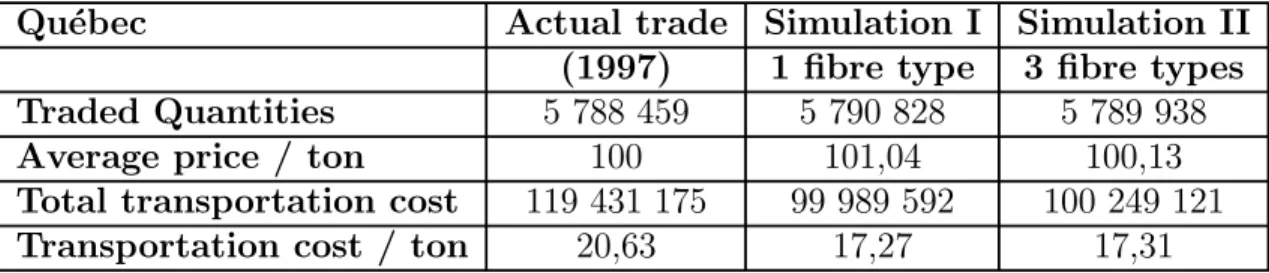
(26) 5.1. Simulation Analyses. Wood chips are a by-product of the production of lumber wood and the major input in the production of paper pulp. The annual sales of wood chips from saw mills to paper mills amounts to some 600M$CND in the Province of Québec alone. Transportation costs account for some 20% of the final wood chip cost. The wood chip market is a multi-product market. Saw mills harvest trees, often of different species. Trees are transformed into lumber wood. The excess wood (wood chips) is retrieved and shipped to paper mills. In a given shipment, wood chips from different species are usually mixed up. On arrival at paper mills, wood chips are weighted and controlled for quality and humidity, and are then stocked according to their fiber content. It is important to note that most (but not all) buyers need to combine the right proportion of high-density and low-density fibers to respect their specific pulp paper recipes. Variations in the proportion of high and low-density fibers reduce the quality of the paper produced. Since buyers typically do not get their wood chips from one source only, they usually combine chips and fibers from different sources for each type of paper produced. There is thus a clear benefit to design auctions that allow bidders to put together efficient combinations of products at the lowest total acquisition and transportation cost. We have used 1997 data provided by the Quebec Department of Natural Resources for the simulations presented herein. The data includes the exact trades in ton between each pair of buyer and seller. In order to calculate the transportation cost between each seller and each producer, we have used a matrix containing the distance in kilometers between each paper mills and saw mills and applied the ongoing market price of 0.11$CND per ton per kilometer. Overall 5,79 million tons were traded betweeen 156 saw mills and 33 paper mills. The total cost for transporting these tons (based on the assumption of an average cost of 0.11$ per ton per kilometer) was 119,4M$CND or an average of 20,63$ per ton, each ton travelling an average of 187,5 kilometers. Simulations are conducted assuming all necessary information is available and that no multi-round auction is required. For each simulation, we generate for each seller and buyer a supply or demand curve. The individual supply curves for each saw mill are generated so that the quantity supplied at price 100$ corresponds to the actual purchased quantity. Similarly, the individual demand curves for each paper mill are generated so that the quantity asked for at price 100$ plus their average transportation cost corresponds to the actual purchased quantity. Hence, the actual trades lie on the respective demand and supply curves. Some assumptions were made for the demand and supply elasticities. However, the elasticity assumptions had little effects on the results of the simulations. For the first set of simulations, we assumed that all units are equivalent and that the paper mills are indifferent over the sources of their fibre. These simultations yielded an upper bound on the savings that can be acheived by reallocating trades in the absence of constraints on the particular mixtures of wood chips required by buyers. For the second set of simulations, we assumed that each buyer desires to maintain the same proportions of fibres as currently. Estimates of the proportions of high-density, low-density fibers, and grey 22.

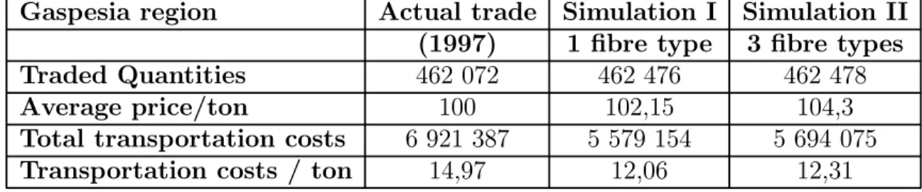
(27) pine fiber sold by each saw mill depend of the origin region of the lumber and were available. Hence, we could estimate the proportion high-density, low-density fibers, and grey pine fiber purchased by each paper mill. We imposed that these proportions be preserved. Since, in practice, paper mills are somewhat more flexible, these simultations establish a lower bound on the savings that can be acheived by reallocating trade. The results of the simulations ´ market are presented in the Table 2. Quantities are in tons, prices in for the entire Qubec Canadian dollars. Qu´ ebec. Actual trade Simulation I Simulation II (1997) 1 fibre type 3 fibre types Traded Quantities 5 788 459 5 790 828 5 789 938 Average price / ton 100 101,04 100,13 Total transportation cost 119 431 175 99 989 592 100 249 121 Transportation cost / ton 20,63 17,27 17,31 Table 2: Simulations of Entire Market Results show overall savings of around 16% in transportation costs per ton. These savings correspond to around 19M$. Results do not vary significantly from Simulation I to Simulation II. The average price per ton displayed in the table corresponds to the price received by the producers. Consequently, compared to the actual trade, producers receive a marginaly higher price, while buyers pay on average somewhat lower prices as transportation costs go down. The results show that savings are shared by producers and buyers, the buyers receiving most of the saving in Simulation II. ´ It is not unreasonable to envision that it could be difficult to bring all the mills of Qubec into a unique market. Therefore, we have simulated a smaller region and number of firms and explored the potential savings in this case. We used data from the five paper mills and their ´ suppliers within the region of Gaspesia, a remote region in Eastern Qubec. We have fixed the trade flows among these firms and those outside the region and considered exclusivelly the reallocation of trade within the region. Table 3 presents the results of these simulations. Only the data related to the trade within the region is presented. Similar results to the previous experiment are observed. Savings around 18% to 19% in transportation cost per ton are observed. Compared to the benchmark, producers receive a higher price. Buyers pay on average lower prices in Simulation I but higher prices in Simulation II as savings in transportation costs are upset by the increase in the price paid to producers.. 5.2. Strategic Analysis of the Market Game. From a game-theoretical point of view, the process defined by the rules presented in this paper is hard to analyze. Actually, there is no formal theory about how players interact in a double-sided market with decreasing demand curves and increasing supply curves. However, there are a few known things about this type of games that allow us to address a number 23.

(28) Gaspesia region. Actual trade Simulation I Simulation II (1997) 1 fibre type 3 fibre types Traded Quantities 462 072 462 476 462 478 Average price/ton 100 102,15 104,3 Total transportation costs 6 921 387 5 579 154 5 694 075 Transportation costs / ton 14,97 12,06 12,31 Table 3: Simulations of Restricted Market of design issues. The main issue is whether the proposed design indeed leads to an efficient allocation of resources and, if not, whether there exist alternative designs that are preferable. The mechanism proposed in this paper leads to the efficient allocation, if the following conditions hold: (i) participants truthfully reveal their preferences (cost and demand functions, transportations costs, quality evaluation) and (ii) their preferences can be represented within the restrictions imposed by our design. Regarding the latter, we believe that for most commodity markets, marginal costs are increasing while marginal user values are decreasing. When the representation of preferences and cost structures does not match what is proposed in this paper, the design can be modified. An extreme example is offered by the electricity market where significant non-convexities exist in the production functions. In this case, we would have to modify both the operations research methodology used to optimize the market and the rules defining how bids may be modified. Most markets do not present such extreme conditions, however, and the required design modifications, if any, are much more benign. The first condition is more troublesome and, in general, one cannot assume it. In particular, when participants are strategic and large enough to have an impact on the equilibrium prices, then revealing one’s true demand or supply schedule is a dominated strategy. It is well known that demand (or supply) reduction is a best response against a downward slopping excess demand curve (Ausubel and Cramton 1996). If one reduces its demand at the margin, it reduces the price one needs to pay on all sub-marginal units. At the margin, the benefit of lowering the price outweighs the cost of buying fewer marginal units. Demand reduction and supply reduction leads to fewer trade than what will be socially optimal and, clearly, there will be unexhausted trade gains in the market. This discussion raises two new questions: (i) to what extent the welfare loss is important and (ii) does there exist alternative mechanisms that will do better? It appears that no definitive answers to these questions exist. The extent of the welfare loss depends on the degree of competition. If the market is perceived as very competitive, the participants will not be able to impact prices much and will tend to limit supply and demand reduction. Similarly, it is hard to imagine that one alternative rule will always do better in all circumstances. However, we know that a mechanism that always implements the efficient allocation must generate negative expected returns to the auctioneer (Myerson and Satterthwaite 1983). In other words, a practical mechanism that always induces efficiency simply does not exist. One may consider alternative multi-round auction processes, different pricing rules, or sequential 24.

(29) trading mechanisms, the issues of bid and market manipulation will arise still. In the process of our study, we have run a number of market experiments. We hired eight students who participated to market experiments over a series of sessions. Each participant was assigned a role, buyer or seller, and was given a cost or demand function. Participants would negotiate using the optimized marketplace and multi-round auction. After 5 rounds, the negotiation would end and the equilibrium prices and quantities were determined. Each participant was paid according to its gains from trade in the market game. Various experiments were conducted by varying the numbers of buyers and sellers, by allowing for communication between participants, etc. We ran no replication, so the evidence remains not statistically valid. Nevertheless, it confirms the above strategic analysis. With a small number of players, participants seek to manipulate prices by asking or offering less than they would if they were non-strategic. In conclusion, the multi-lateral optimized market design proposed in this paper will not lead to full efficiency if participants have market power and are strategic. However, there exists no alternative design that will induce efficiency in this context, either. On the other hand, when competition prevents participants from seeking to manipulate the market to alter equilibrium prices, the proposed periodic optimized multi-lateral multi-commodity market is designed to maximize gains from trade given the transportation costs and technical constraints of the industry.. 5.3. Difficulties in Implementing an Optimized Market. The previous discussion leads to two conclusions: (i) Simulations for the wood chip industry indicate that substantial savings could be obtained; (ii) Game theory and experiments point to the fact that strategic bid manipulations leading to inefficiencies will occur unless the number of participants is sufficiently large. Hence, optimized markets are worthwhile, from an efficiency point of view, only if a large number of traders accept to participate. Our ´ wood chip market tells us that regrouping a large number of experience with the Qubec self-interested parties around a smart market is not an easy undertaking. A marketplace is valueless to sellers if there are no participating buyers and it is valueless to buyers if there are no sellers. The first difficulty is to create the necessary critical mass to make it worthwhile. If there are too few buyers and sellers the market remains illiquid and gains from trade will not be large enough. So, how to create the critical mass? It could be done by general consensus within the industry, it could be imposed by the regulator, or it could be done within a large and decentralized corporation that wishes to coordinate intra-organizational trade among its various branches. The second difficulty is that firms in general do not care about efficient markets. They care about being efficient in a inefficient market. When markets are inefficient, it is costly to identify profitable gains from trade and more talented intermediaries can achieve extra 25.

(30) profits. So, naturally, firms invest a lot in market knowledge that could potentially provide them with a competitive advantage. They are unlikely then to move towards a market environment that would render their investment obsolete. One feature of an efficient market is that information on equilibrium prices is readily accessible, lowering bilateral negotiation costs. In our discussion with the paper mills, they clearly stated that they did not want to join a marketplace, optimized or not, that would provide information on prices. Accordingly, the operator of an electronic marketplace would have a better business model, if it offers a simple trading device (where eventually the negotiated prices remain known only to the involved parties) and offers added value services to each individual participant that wishes to pay an extra fee for improved marketing services. Such an offering remains far from the so-called optimized markets. Despite these previous comments, we believe that the concept of optimized markets will prove fruitful in the long run. Business-to-business electronic commerce seems to move progressively towards a more collaborative environment where firms seek to optimize their joint efficiency and supply chain. A centralized optimized market may serve as a way to achieve this. When markets remain decentralized, a centralized optimized market model may serve as a useful benchmark. Decentralized optimized market mechanisms can also be developed. But these developments are well beyond the scope of the present paper.. 6. Conclusions. We presented a design for an optimized, centralized, multi-lateral, periodic commodity market where all possible multi-lateral trades are solved simultaneously. Commodities are non homogeneous and are classified by type or quality. Sellers may offer several commodity types separately or mixed up in lots. Buyers need to combine different grades and qualities and, consequently, have to trade with several buyers. Since the complementary commodities are needed as input to the same process, these trades have to be performed simultaneously. Technological constraints limit the quantities of each type of commodity a buyer may acquire. Transportation costs are significant but commodities do not have to pass through a hub on their way from sellers to buyers. The market clearing mechanism includes explicit optimization tools that seek to allocate resources efficiently, that is to optimize both the production and transportation of resources in the industry. Given the information available, the market mechanism identifies an “optimal” allocation, which indicated who sells what what to whom, as well as prices, who pays what to whom. We have detailed the operations research models and the mathematical programming methods required for the efficient computation of the market equilibrium Since industry participants are usually unwilling or unable to disclose all the pertinent but very personal and proprietary information required for such an optimized market, we also introduced a multi-round auction process that requires significantly less a priori information 26.