Backhauling optimization for a wood recycling company

(1)

© Maxime Leclerc, 2020

Backhauling optimization for a wood recycling company

Mémoire

Maxime Leclerc

Maîtrise en génie mécanique - avec mémoire

Maître ès sciences (M. Sc.)

(2)

Backhauling optimization for a wood recycling company

Mémoire

Maxime Leclerc

Sous la direction de:

Mikael Rönnqvist, directeur de recherche

Jean-François Audy, codirecteur de recherche

(3)

iii

Résumé

Les coûts de transport représentent une grande partie des coûts d'exploitation des entreprises de recyclage du bois. Le problème que nous étudions est le problème du transport avec retour en charge, au sein duquel une entreprise doit décider comment connecter ses points d'approvisionnement et de demande en utilisant des itinéraires. Dans ce mémoire, le problème résolu est un cas particulier du problème de transport dans lequel le producteur n'a qu'une seule usine. Ce cas spécial est rarement étudié dans la littérature scientifique. Nous utilisons un modèle de programmation linéaire pour résoudre ce problème. Nous présentons les résultats obtenus lorsque nous appliquons cette approche aux données d’une entreprise de recyclage du bois. Nous étudions l'effet de l'horizon temporel de planification en comparant la planification annuelle des transports à la planification hebdomadaire. Nous comparons aussi l’effet de différents calculs de distance, différents types de camion et différents objectifs d’optimisation. Les résultats montrent 42% d'économies de temps de déplacement pour la planification annuelle et 36% d'économies pour la planification hebdomadaire. Nous analysons également la répartition des économies entre un ensemble de transporteurs et rapportons que 49% des économies impliquent le transporteur priorisé par la société de recyclage. Lorsque nous ajoutons des contraintes aux types de camions pouvant effectuer des retours en charge, les économies chutent à 17%. Ces contraintes résultent du fait que les entreprises de recyclage du bois utilisent différentes catégories de matériaux et nécessitent par conséquent des configurations de camions spécifiques. Enfin, une analyse des coûts de transport et des revenus de la société de recyclage montre que notre modèle peut potentiellement augmenter considérablement les revenus de transport.

(4)

iv

Abstract

Transportation costs represent a large portion of the operation costs for wood recycling companies. The problem we study is the transportation with backhaul problem in which a company must decide how to connect its supply and demand points using routes. In this master’s thesis, the problem solved is a special case of the transportation problem where the producer only has one mill. This special case is rarely studied in the scientific literature. We use a linear programming model to solve these problems. We present results obtained when applying this approach to data from a wood recycling company. We investigate the effect of the planning time horizon by comparing yearly transportation planning against weekly planning. We also compare the effect of different distance calculations, different types of trucks and different optimization goals. The results show 42% in traveled time savings for yearly planning and 36% in savings for weekly planning. We also analyse the distribution of the backhaul savings among a set of carriers and report that 49% of the savings involved the recycling company’s prioritized carrier. When we add constraints on truck types that can perform backhauls, savings drop to 17%. These constraints result from the fact that wood recycling companies handle different categories of materials and therefore require specific truck configurations. Finally, an analysis of the recycling company’s transportation costs and revenues show that our model has the potential to substantially increase transportation revenues.

(5)

v

List of figures

Figure 1. Direct and backhaul routes comparison. ... 5

Figure 2. Constraints and feasible region for the dual price example [19]... 13

Figure 3. Relaxing constraint 1 by adding one additional available unit on the right-hand side increases the maximum profit by $3.40 [19]... 14

Figure 4. Input supply S and demand D site map for the numerical example. ... 15

Figure 5. Mapping of the direct routes R for the example solution. ... 17

Figure 6. Direct and backhaul routes map for the example solution. ... 18

Figure 7. Heatmap input data... 19

Figure 8. Heatmaps solution. ... 20

Figure 9. Heatmap route distances analysis. ... 21

Figure 10. Digital Elevation Model [22]. ... 22

Figure 11. Generating Road Altitudes Algorithm. ... 23

Figure 12. Supply sources of recycled wood include the construction, renovation and demolition sector, wood fences and chairs makers, and eco-centers [24] [25] [26]. ... 25

Figure 13. Clients of recycled wood include the bioenergy sector, farmers and construction materials [27] [28] [29]. ... 25

Figure 14. Backhaul routes. ... 26

Figure 15. Flows from WRC’s suppliers to WRC. ... 27

Figure 16. Flows from WRC to its clients. ... 28

Figure 17. Map of WRC clients (full circles) and suppliers (empty circles). ... 51

Figure 18. Map of potential sites. ... 52

Figure 19. Dual price heatmap for new suppliers. ... 53

Figure 20. Dual price heatmap for new suppliers as well as current customer locations. ... 54

Figure 21. Dual price heatmap for new clients. ... 54

(9)

ix

List of tables

Table 1. Supply and demand products and quantities qs for the example... 15

Table 2. Direct routes R, sites visited dr, flows fr and costs cr for the example solution. ... 16

Table 3. Direct R and backhaul B routes, sites visited dr / kb, flows fr / wb and costs cr / ob for the example solution. ... 18

Table 4. Problem instances. ... 31

Table 5. General statistics for WRC transportation. ... 37

Table 6. WRC direct and backhaul routes results for the four problem instances using as the crow flies’ distances (ATCFD). ... 38

Table 7. Top 5 backhaul routes that generate the most savings for problem instance 2... 38

Table 8. Top 15 backhaul routes that generate the most savings for problem instance 2. ... 39

Table 9. WRC direct and backhaul routes results for the three problem instances using real travel time estimates (RTTE). ... 41

Table 10. Travel time and truck loads without backhauls. ... 45

Table 11. Travel time and truck loads with backhauls using as the crow flies’ distances ATCFD. ... 46

Table 12. Costs and revenues without backhauls. ... 46

Table 13. Costs and revenues with backhauls. ... 46

Table 14. WRC direct and backhaul routes results for the two transportation costs and revenues problem instances. ... 46

Table 15. WRC direct and backhaul routes results synthesis for the seven problem instances. ... 47

Table 16. Backhaul savings distribution among carriers. ... 48

(10)

x

Acknowledgements

I would first like to thank my thesis advisors Mikael Rönnqvist at Université Laval and Jean-François Audy at Université du Québec à Trois-Rivières for the continuous support of my graduate studies and related research, for their patience, their motivation, and for their immense knowledge. I could not have imagined having better advisors or mentors for my graduate studies. Their office door was always open whenever I had a question about my research or writing. Their guidance helped me in all the time of research and writing of this thesis.

I would also like to thank the controller and the operations director at the partner Wood Recycling Company who were involved in the validation for this research project. Without their enthusiastic participation and input, the validation could not have been successfully conducted.

I am grateful to my fellow graduate students for the stimulating discussions, their feedback, their cooperation, their friendship and for all the fun we have had in the last years.

I would like to acknowledge the financial support of the Canada Research Chair in Operations Research in Natural Resources and NSERC Engage grants for the scholarships that I was granted. Finally, I must express my very profound gratitude to my parents, family and friends for providing me with love, unfailing support, continuous encouragement, wise counsel and sympathetic ears through my years of study, through the process of researching and writing this thesis and through my life in general. This accomplishment would not have been possible without them. Thank you.

Quebec City, August 2020 Maxime Leclerc

(11)

1

Introduction

In the business of wood recycling, costs are split between labor, maintenance, raw materials, and supply chain. Transportation accounts for a significant part of the logistics costs in the wood recycling supply chain. In this work, we partnered with a Wood Recycling Company (WRC). We will follow best practice and mask the name of our partner.

The goal of this thesis is to analyse WRC’s transportation costs and to offer recommendations concerning which geographic areas WRC should prioritize when it looks for new partners. Achieving this second objective will greatly help WRC to decide which partners are the most attractive when we also consider the location of their current partners. Using this information can generate large cost savings for WRC.

The company studied in this master’s thesis does not currently use decision support tools to coordinate and minimize its transportation costs. By reducing overall travelled distances and traveling time using optimization tools, we generate transportation cost savings for the recycling company. More precisely, we can use backhauls to reduce the unloaded truck distances.

Using a linear programming model, we compare the effect of planning yearly versus planning weekly. In addition, we compare the effect of different distance calculations, different types of trucks and different optimization goals. We also investigate the effect of carrier collaboration on costs and how the savings are split among carriers. Using dual price heatmaps, we provide suggestions to our partner company concerning where it should look for new clients or suppliers. In the context of this thesis, the studied Wood Recycling Company WRC has only one plant as opposed to the previous articles where multiple plants are modeled. In addition, all routes start from WRC and end at WRC. As a result, our model can benefit from these simplifications.

When reviewing the literature, we see that backhauls created savings from 6% up to 37%. The variation in savings is a function of the different model assumptions each author uses.

We obtain 42% in traveled time savings for yearly planning and 36% in savings for weekly planning. In addition, we report that 49% of the savings involve the recycling company’s favoured carrier. Wood recycling companies handle different categories of materials and as a result require specific truck

(12)

2

configurations. Savings are reduced to 17% when we constrain which truck configurations can perform backhauls. These savings can be superior to 17% if we change the current carrier usage. Finally, results show that our model has the potential to significantly increase transportation revenues. This thesis is organized as follows. We first give some context information about wood recycling and transportation and a detailed problem description. Next, we present a literature review covering backhauling for the wood industry, followed by the linear programming models and route generation methods we used. Afterwards, we describe the recycling company and our practical case study that uses our models. In this chapter, we detail the problem instances and analyses that were prioritized to help our partner make informed transportation decisions. The chapter discusses how we can vary the constraints on the backhaul routes generated, analyse how savings are split, and generate transportation cost heatmaps. Finally, we present our results, a discussion, a summary, and our conclusions.

(13)

3

Chapter 1 Problem description

1.1 Recycling industry

Recycling is the process of converting discarded materials into new materials. According to Recyc-Quebec, the “2.5 million tons of the most commonly recycled residual materials recovered in Quebec in 2006 (metal, paper, cardboard, plastic, and glass) were valued at $550 million and generated over 10,000 direct jobs” [1]. Statistics Canada [2] reports that “the amount of waste diverted to recycling or organic processing facilities decreased by 3% from 2008 to 8.1 million tonnes, or 236 kg per person in 2010. This decrease, which was the first since 2002, was fueled by an 11% decrease in non-residential waste diversion. In contrast, residential waste diversion increased by 5%”.

Recycling and reintroducing recycled materials into the production cycle also yield significant gains with respect to the economy, resource protection, and greenhouse gas emissions reduction. These recycled materials were previously deemed unrecoverable and buried. They are now transformed into quality products for different customers. In some cases, adding recycled material can also increase product quality.

1.2 Transport industry

Transport Canada [3] projects that transportation of wood commodities including recycled wood will grow moderately over the next ten years. Transport and warehousing represent 4.5% (or $75 billion) of Canada’s Gross Domestic Product and 5% (or 897,000) of Canada’s jobs. The sector grew by 3% in 2016. This growth rate was more than double of the growth rate for all industries.

Transport Canada [3] reports that road transportation was responsible for 83.5% of transport-related greenhouse gas emissions in 2016. It has increased its emissions over the last ten years because of increasing traffic. According to Statistics Canada [2], total factor productivity (TFP) in the transportation and warehousing sector has increased by an average of 0.4% yearly from 1986 to 2015, compared to 0.1% for the overall business sector.

(14)

4

Transport Canada [3] also reports that “there are more than 1.13 million two-lane equivalent lane-kilometres of public road in Canada. Approximately 40% of the road network is paved, while 60% is unpaved. Four provinces—Ontario, Quebec, Saskatchewan, and Alberta — account for over 75% of the total road length.”

According to Transport Canada [3], the number of companies whose primary activity was trucking transport was 66,751 in 2016. Quebec was home to 15.1% (or 10,079) of these businesses. In 2015, around 4.4% (or 1.05 million) of the total 23.9 million road motor vehicles registered in Canada were medium and heavy trucks weighing 4,500 kilograms or more. In 2016, trucking traffic amounted to 276 billion tonne-kilometres.

Over the next few years, we can expect significant progress in automated and unmanned vehicle technologies [4] from companies such as Amazon, Apple, Google, NVIDIA, Otto, Tesla, Uber, etc. Quebec, Ontario, Alberta, and British Columbia currently host the testing of automated vehicles. Many vehicle manufacturers and researchers including Ford Canada, GM Canada, and Uber Toronto are conducting research on autonomous vehicles. In addition, the transition to digital books, music and movies could change the demand for transportation.

Transport Canada [3] adds that “an aging population leads to more workers retiring, skill shortages will likely be an issue moving forward. The need to recruit, train and retain workers in the transportation sector, especially in the marine and trucking industries will increase as competition for skilled employees grows.”

In this multifaceted context, operational research planning methods allow us to appraise the maximum transportation costs savings potential (the upper bound) for transportation problems.

1.3 Backhauling in the wood industry

The problem we explore in this thesis is named transportation planning with backhaul. In a more general setting, a Vehicle Routing Problem (VRP) can assign complex routes to a specific truck. In addition, the VRP can handle multiple mills. The problem we will solve is less common and a special case of the transportation problem where the producer only has one mill. The vehicle routing problem

(15)

5

is a generalization of the Travelling Salesman Problem (TSP). In the TSP, a travelling salesman (or vehicle) must visit several nodes exactly once [5]. These nodes can represent the set of clients and/or the set of suppliers. The salesman must perform a tour that starts from a node, visits all the other nodes, and returns to the original node. The goal is to find the shortest tour. In the VRP, we generalize the TSP by having many salesmen or vehicles. For the VRP, we need to find the optimal set of routes that visit all the nodes exactly once [6]. In addition, flows, measured in truck load units, correspond to each route. These flows ensure that supplies are collected and that demands are met.

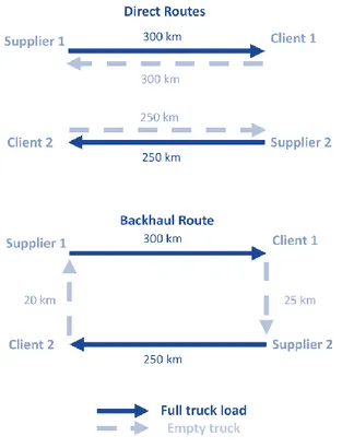
Figure 1 illustrates the difference between direct and backhaul routes. We can see that the full truck load distance is the same for both situations: 300 km + 250 km = 550 km. However, by exploiting the fact that Client 1 and Supplier 2 are nearby (and the fact that Client 2 and Supplier 1 are close to each other), the distance travelled while the truck is empty is reduced.

Figure 1. Direct and backhaul routes comparison.

For direct routes, the total empty distance is 550 km. However, for the backhaul route, the empty distance is 25 km + 20 km = 45 km. In addition, the total distance travelled is also reduced from 1,100 km to 595 km using the backhaul route.

(16)

6

In the context of this thesis study, there is only one plant. As a result, we label and define Supplier 1 so that it corresponds to the plant. Client 1 will be the destination WRC delivers its recycled wood products. Supplier 2 will be the supply point where WRC picks up used wood to be recycled. Finally, Client 2 will correspond to the location where the used wood is delivered, which is at WRC’s plant. As a result, Supplier 1 and Client 2 are both located at WRC’s address. In addition, there is no empty truck load distance between these two nodes.

Compared to the VRP, the VRP with backhaul (VRPB) adds the following requirement which is illustrated in Figure 1. Each vehicle aims to start by picking up a truck load from Supplier 1 (the plant) and delivering the truck load to Client 1 (an outbound flow, from the plant). The vehicle then picks up a truck load from Supplier 2 and delivers the truck load to Client 2 (the plant, which receives an inbound flow).

In order to convert two separate pickup and delivery sequences in a single backhaul route, we must ensure that both sequences in Figure 1 can be performed with the same truck. This means that both types of transported goods (wood to be recycled and recycled wood product) can be moved with the same truck type. Combining two different deliveries can sometimes lead to cleaning costs to avoid mixing the two types of goods.

As shown in Figure 1, backhaul routes allow trucks to minimize the total distance they travel, especially the distance they travel while they are empty. Backhauling therefore reduces total transportation costs. Backhauls are also interesting for companies that want to mitigate their environmental impact by minimizing their fuel consumption and associated greenhouse gas emissions.

In practice, this thesis will study a variation of the VRP with backhaul problem: the transportation planning with backhaul. Since our partner has only one mill, each backhaul routes will visit in order the following three sites: the routes will start at the mill, visit a client, visit a supplier, and return to the mill. In addition, we will use a fast and exact method instead of heuristics to solve the backhauling problem.

(17)

7

Chapter 2 Literature review

2.1 The backhauling problem

The following papers present the evolution of backhauling through time. In these papers, we see that backhauls created savings varying from 6% up to 37%. The difference in savings results from the changes in the model assumptions from one paper to another. We start by covering the backhaul literature in general. We then move on to cover backhaul usage for the wood industry. The methods used in the following papers include various heuristics, problem decompositions, column generation and branch-and-bound techniques, clustering algorithms, optimization programs, GIS databases, and road databases.

Lundgren et al. [5] present general optimization theory that will be used in this thesis. In particular, the book’s section 5.3 defines a dual price as “the change in objective function value when making a marginal increase of the [constraint’s] right hand side”. Using dual prices will allow us to reach our goal of recommending geographical areas where WRC should find new partners. We cover dual prices in more details in this thesis’ section 3.2.

Jordan [7] developed a model to help coordinate backhauling between more than two terminals. He tested two heuristics for this backhauling problem: a matching formulation and a Lagrangian relaxation. As a result, he reduced empty truck distances in his case studies by 37% compared with the solutions that did not use backhauls.

Min et al. [8] created an optimization model for backhauls involving multiple capacitated vehicles and depots. They decomposed the problem into three phases and sub-models. The first phase involves clustering customers and vendors. The second phase designs aggregated routes and assigns clusters to depots using a binary integer program. The third phase creates individual routes by solving traveling salesman problems.

Bailey et al. [9] also tested two heuristics for backhauling: a greedy heuristic and a tabu search. They obtained transportation cost savings of 27% when they used backhauling. They found that the resulting backhaul routes depended on the transporter collaboration fees.

(18)

8

Pradenas et al. [10] studied backhauls with the objective or reducing the emission of greenhouse gases. They observed that it is possible that both the amount of fuel consumed, and the required energy decrease while both the distance travelled, and the transportation costs increase. In addition, they found that cooperation among transportation companies decreased by approximately 30% overall pollution and costs for each company involved. Similarly, Juan et al. [11] studied the positive impact of cooperation and backhauls on transportation costs and CO2 emissions.

2.2 Backhauling in the wood industry

Puodžiūnas et al. [12] used a backhauling optimization model to coordinates various forest enterprises on a tactical level. They used a column generation algorithm to reduce the computational complexity. They observed that up to 56% of the transported volume could be included in backhauls. The net effect on transport costs savings resulted in a potential upper bound of 16% when the involved companies agreed to coordinate their effort.

Forsberg et al. [13] created a linear programming backhaul optimization model named FlowOpt for Swedish forest companies with a customizable planning horizon. The system includes a tactical planning of backhaul routes, a GIS map user interface, and a road database. FlowOpt facilitated case studies by improving the planning speed, the result quality, the modelling precision, and sensitivity analyses. It also led to increased coordination and integration. Similarly, Palander and Väätäinen [14] studied the impact of backhauling and collaboration for wood companies. They found they could reduce transportation costs by 20.4%.

Carlgren et al. [15] developed an integrated backhauling integer programming model for forest companies using fast column generation and branch-and-bound techniques. As a result, they were able to reduce costs by 25%. In addition, they found that it is advantageous to cover a large geographical region and to have a diverse mix of products to obtain maximum backhauling savings. Carlsson and Rönnqvist [16] applied tactical backhauls to forestry companies and obtained savings up to 28% by minimizing unloaded traveling distances. They obtained savings in terms of costs and reductions in pollution produced. They use a mixed integer linear programming model to find the optimal routes for a daily to yearly planning horizon. The solution procedure also uses column generation techniques.

(19)

9

Using a different iterative solution procedure, Amorim et al. [17] obtained 6% in backhauling savings for a wood-based panel company. Similarly, Abasian et al. [18] studied tactical backhauling and collaboration for forest companies in order to reduce costs and greenhouse gas emissions using mixed integer programming. They achieved 23% in potential savings.

(20)

10

Chapter 3 Models and methods

3.1 Mathematical model formulation

We present here our linear programming model to find the optimal set of routes. Section 4.2 will detail our route generation technique.

We present our model for the VRPB. The problem solution consists of a list of direct routes and backhaul routes we should use as well as the flows and transportation costs associated with these choices. We base our methods to solve the VRPB on the model and procedure from Carlsson and Rönnqvist [16]. The main difference here is that WRC only has one mill as opposed to many.

Sets

set S = All the supply sites. S1, …, Si. set D = All the demand sites. D1, …, Dj, set R = All the direct routes between the plant and supply or demand sites R1, …, Rk. set B = All the backhaul routes starting from the plant, going to a demand site, visiting a supplier,

and ending back at the plant. B1, …, Bm. sets r_s = All the direct routes that visit supply or demand point s.

sets b_s = All the backhaul routes that visit supply or demand point s.

sets dr = All the supply and demand sites visited by direct route r.

sets k_b = All the supply and demand sites visited by backhaul route b.

General parameters

qs = Supply or demand in full truck load units for each site s from the sets S and D.

c_r = Cost for each direct route r from the set R. o_b = Cost for each backhaul route b from the set B.

(21)

11 Decision variables

f_r = Flow in full truck load units that use direct route r. w_b = Flow in full truck load units that use backhaul route b.

Objective function 𝑚𝑖𝑛𝑖𝑚𝑖𝑧𝑒 𝑧 = ∑ 𝑟 ∈ 𝑅 (c_r∗ f_r) + ∑ 𝑏 ∈ 𝐵 (o_b∗ w_b) Constraints Subject to: ∑ f_r 𝑟 ∈ 𝑟𝑠 + ∑ w_b 𝑏 ∈ 𝑏𝑠 = q_s, ∀𝑠 ∈ 𝑆 ∪ 𝐷

(Each supplier delivers all their supply and each client receives all their demand) f_r ≥ 0, w_b ≥ 0, ∀𝑟 ∈ 𝑅, ∀𝑏 ∈ 𝐵

(The flows must be positive) The details of the route generation used in this thesis is presented in section 4.2 as a part of the case study description.

(22)

12

3.2 Dual prices

One of our goal is to provide suggestions to our partner company about as to where it should look for new clients or suppliers that will foster backhauling opportunities. As a reminder, this information will be essential for WRC in order to decide which partners are the most attractive when we also consider the location of their current partners. Putting these new valuable partners first can generate large cost savings for WRC.

We present these new partner suggestions using heatmaps. To create these heatmaps, we need to compute dual prices which also referred to as shadow prices. Here is a short review covering dual price theory.

We will present an example adapted from [19] to illustrate dual prices. In this example, a company produces two different products. The company’s goal is to maximize its profit. However, the company has limited resources that are modeled using constraints.

Decision variables

X1 = Quantity produced for product 1.

X₂ = Quantity produced for product 2.

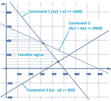
Objective function 𝑚𝑎𝑥𝑖𝑚𝑖𝑧𝑒 𝑝𝑟𝑜𝑓𝑖𝑡 = 8X₁+ 5X₂ Constraints Subject to: 2X1+ X2 ≤ 1000 (Constraint 1) 3X₁+ 4X₂ ≤ 2400 (Constraint 2) X₁ − X₂ ≤ 350 (Constraint 3) X1 ≥ 0, X2 ≥ 0 (Constraints 4 and 5)

(23)

13

Figure 2 illustrates this example problem. First, the constraints are plotted in the figure. Next, the intersection of the region common to all constraints, the feasible region, is striped .

Figure 3 shows the two possibilities for the maximum profit. When we use the original constraints, the maximum profit is $4360. However, when we relax constraint 1 by adding one additional available unit on the right-hand side of the constraint, we increase the maximum profit by $3.40. This increase corresponds to the dual price for this constraint:

𝐷𝑢𝑎𝑙 𝑝𝑟𝑖𝑐𝑒 = 𝐶ℎ𝑎𝑛𝑔𝑒 𝑖𝑛 𝑜𝑏𝑗𝑒𝑐𝑡𝑖𝑣𝑒 𝑣𝑎𝑙𝑢𝑒

𝐶ℎ𝑎𝑛𝑔𝑒 𝑖𝑛 𝑡ℎ𝑒 𝑐𝑜𝑛𝑠𝑡𝑟𝑎𝑖𝑛𝑡 𝑟𝑖𝑔ℎ𝑡 ℎ𝑎𝑛𝑑 𝑠𝑖𝑑𝑒 𝑣𝑎𝑙𝑢𝑒

(24)

14

Figure 3. Relaxing constraint 1 by adding one additional available unit on the right-hand side increases the maximum profit by $3.40 [19].

Similarly, we can test the change in optimal transportation costs for our case study when we increase the demand or supply by one unit. This will be illustrated in the next section, 3.3 Numerical examples.

3.3 Numerical examples

We present here a numerical example with two products, seven suppliers and three demand sites. Input data for the first example

Figure 4 shows the location of supply and demand sites for the example. The supply points are represented with colored triangles. Blue corresponds to pulp supply and green corresponds to saw supply.

Table 1 lists the demand and supply quantities qs for each site. Supply is represented by a negative

(25)

15

Figure 4. Input supply S and demand D site map for the numerical example.

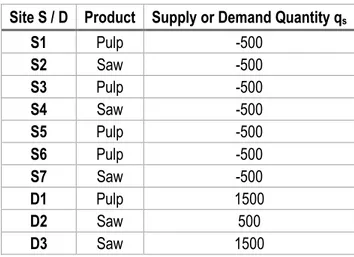
Table 1. Supply and demand products and quantities qs for the example. Site S / D Product Supply or Demand Quantity qs

S1 Pulp -500 S2 Saw -500 S3 Pulp -500 S4 Saw -500 S5 Pulp -500 S6 Pulp -500 S7 Saw -500 D1 Pulp 1500 D2 Saw 500 D3 Saw 1500

(26)

16 Handling different product categories

We mentioned previously that our case study involves full truck loads of different product categories (inbound products to the plant and outbound products from the plant). The example in this section also has more than one product category. To make sure that each demand site receives the correct product category, we list the product category for all the demand and supply sites. This information is then used by our route generator. The generator makes the following verification: when a route picks up a full truck load from a supply site and delivers this load to a demand site, the product type for both supply and demand sites must be the same.

Solution for the first numerical example

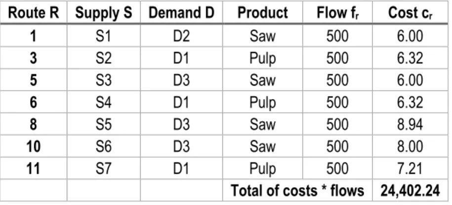
Here is the solution using only direct routes. Table 2 lists the direct routes R, their visited supply and demand sites dr, the route flows fr, and the route costs cr. We see that the total cost is 24,402.24. Figure

5 maps the direct routes used to minimize transportation costs.

Table 2. Direct routes R, sites visited dr, flows fr and costs cr for the example solution. Route R Supply S Demand D Product Flow fr Cost cr

1 S1 D2 Saw 500 6.00 3 S2 D1 Pulp 500 6.32 5 S3 D3 Saw 500 6.00 6 S4 D1 Pulp 500 6.32 8 S5 D3 Saw 500 8.94 10 S6 D3 Saw 500 8.00 11 S7 D1 Pulp 500 7.21

(27)

17

Figure 5. Mapping of the direct routes R for the example solution.

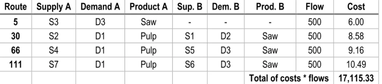
The solution using direct and backhaul routes is presented next. We see in Table 3 that the total cost is 17,115.33. This represents savings of 42.58%. Figure 6 maps the direct and backhaul routes used to minimize transportation costs. The optimization model exploits the fact that it is advantageous to avoid travelling with an empty truck especially when it is possible to travel to a nearby supply site after performing a delivery. This happens twice for the backhaul route in which we travel with an empty truck from D1 to S1 and from D2 to S2. This also happens twice for the backhaul route in which we travel from D1 to S5 and from D3 to S4. The same situation presents itself for the backhaul route in which we travel from D1 to S6 and from D3 to S7.

(28)

18

Table 3. Direct R and backhaul B routes, sites visited dr / kb, flows fr / wb and costs cr / ob for the example solution.

Route Supply A Demand A Product A Sup. B Dem. B Prod. B Flow Cost

5 S3 D3 Saw - - - 500 6.00

30 S2 D1 Pulp S1 D2 Saw 500 8.58

66 S4 D1 Pulp S5 D3 Saw 500 9.16

111 S7 D1 Pulp S6 D3 Saw 500 10.49

Total of costs * flows 17,115.33 Figure 6. Direct and backhaul routes map for the example solution.

(29)

19

Input data for the second example (heatmaps)

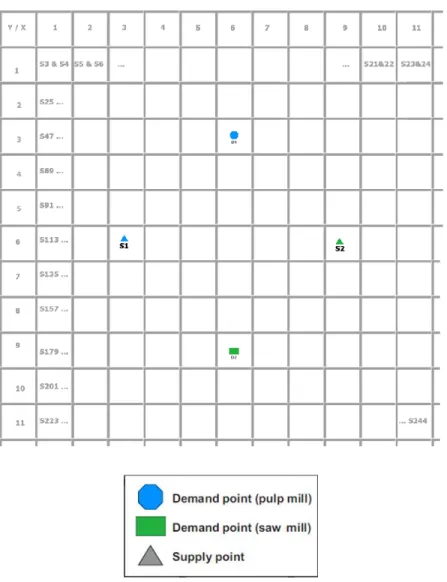
We present a second example to illustrate the problem of generating dual price heatmaps. In this problem, we use two regular demand points and two regular supply points. We use the same site colors as in the previous example: blue represent pulp sites and green represent saw sites. In addition to these four points, we investigate what would be the effect on transportation cost if we would have access to new supply sites. As a result, we create 11 * 11 = 121 additional supply points for each product (pulp and sawmills): S3 to S244.

(30)

20

Heatmaps generation solution for the second example

We perform our analysis using shadow prices which are defined as follows: “The shadow price for a constraint is given by the change in the objective function value when making a marginal increase of the right-hand-side.” [5] For our example, this means that if we increase the right-hand-side of our new supply constraint, the shadow price tells us how much transportation costs will increase or decrease. In section 3.1, we presented the supply constraints. The supply quantities qs were negative numbers:

∑

𝑟 ∈ 𝑑𝑟

f_r+ ∑

𝑏 ∈ 𝑘𝑏

w_b = q_s, ∀𝑠 ∈ 𝑆 ∪ 𝐷

We can therefore expect that if we make qs more positive, this will result in less supply and, as a result,

in higher transportation costs. This means that the shadow price of interesting supply points will be positive, and the shadow price of less interesting supply points will be close to zero.

This is illustrated in Figure 8. The resulting figure on the left is for pulp products and the figure on the right is for saw products. We see that for pulp products, it would naturally be advantageous to have pulp supply points near the pulp demand site at the top. In addition, we see that potential pulp supply points near the saw demand point at the bottom could be interesting since they would create backhaul routes. The same logic applies for saw products when examining the second figure on the right. Figure 8. Heatmaps solution.

(31)

21

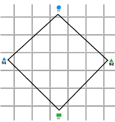
Figure 9 provides additional information on the heatmap example. If we compute the backhaul route distance using the four original sites, we get 4(32_{+ 3}2₎1₂_{= 4(4.24) = 16.96. This corresponds}

to the following route: S1, D1, S2, D2, and S1. If we now add a new pulp supply site, S3, located where D2 is, the new backhaul route becomes S3, D1, S2, D2, and S3. The new backhaul route distance becomes 6 + 4.24 + 4.24 + 0 = 14.48. As a result, we get a reduction of 2.48 distance units with the addition of the new pulp supply site S3. This explains why it would be advantageous to add a new pulp supply site near the saw demand site.

(32)

22

3.4 Generating road altitudes

To generate distances, we need to provide our distance calculator software with the network of roads that can be used. Addresses Quebec (AQ) [20] is a geographic road database that covers all of Quebec. It offers a complete road network including official road names, addresses, route management information, postal codes, and map context. This database is widely used by researchers and professionals. An important drawback of the AQ database is that it does not contain any information about the altitude or Z coordinate for the roads. For this project, we aim to have accurate fuel consumption for our routes. To compute this consumption, we do need road altitudes.

Fortunately, we have access to a separate database that stores the altitude or Z coordinate for a large portion of the Province of Quebec territory. Figure 10 compares the two types of Digital Elevation Models. Digital Surface Models include the earth's surface all objects on the surface. Digital Terrain Models represent the uncovered ground surface without any objects. Since our Digital Elevation Model (DEM) [21] database do not contain information about roads, we need to merge its altitude data with the AQ database. The steps presented in Figure 11 and below are used to perform the merge using ArcGIS version 10.4.

(33)

23 Figure 11. Generating Road Altitudes Algorithm.

1) Merge the collection of DEM map pieces into a single combined real raster matrix. 2) Convert the real raster matrix data into an integer vector polygon format.

3) Update the AQ road polylines altitudes using the shape interpolation algorithm. 4) Reduce the size of the resulting road database using the simplify line algorithm. Here is a more detailed explanation of the road altitude generation algorithm:

1) The DEM database is stored into small map portions that cover the Province of Quebec territory. As a result, we need to merge the collection of DEM raster pieces into a single combined raster.

2) We next convert the real raster matrix data into an integer vector polygon format.

We need this conversion since the original format of the DEM database cannot be used directly in the next processing step: the input data must be in vector polygon format for the shape interpolation algorithm.

3) We update the AQ road polylines altitudes using the ArcGIS shape interpolation algorithm. 4) We finally reduce the size of the resulting road database using the ArcGIS simplify line

algorithm.

This last step is required because the distance and fuel consumption computation algorithms cannot efficiently handle road networks that are too large or too complex. As a result, we reduced the network size from 2 gigabytes to 400 megabytes for this project.

(34)

24

The resulting new road database was also used by other related research projects such as [23]. In Quebec, Canada, wood companies generally pay their transporters according to the time taken to complete a trip from a place of origin (the wood supply zone) to the destination (the processing plant, or the clients). This hourly transportation rate takes fuel consumption into account but, for most companies, the fuel consumption remains a rough approximation of the real consumption.

In [23], an improved version of a fuel consumption model is proposed with the aim of providing a more accurate estimate of fuel consumption. Reductions in greenhouse gases emissions depend on this fuel consumption. The paper’s model considers different characteristics of the road network that affect fuel consumption such as elevation profile, intersections, acceleration, and deceleration due to road signs. The Addresses Quebec road network is used in a routing software which integrates all the characteristics of the road network considered by the consumption model. This had never been done before for the Addresses Quebec road network. By using these consumption models and road networks, it is possible to calculate more precisely and with greater accuracy the fuel consumption in wood road transport, the duration of trips and the reductions in greenhouse gases emissions.

(35)

25

Chapter 4 Company and case study

4.1 Company presentation

Our partner for this project is a private company that we will name Wood Recycling Company (WRC). WRC is a specialized company created in 2011 and recognized for the quality of its products made from recycled wood.

In Figure 12, we present a few of the supply sources of recycled wood. On the left, we show an example of the wood supplied by the construction, renovation, and demolition sectors. In the center, we display a wood fence and wood chairs: their production often results in bits of wood that can be recycled. On the right, we show an eco-center. These centers accept wood wastes from the local population. Figure 12. Supply sources of recycled wood include the construction, renovation and demolition sector, wood fences and chairs makers, and eco-centers [24] [25] [26].

Figure 13 presents three types of customers of recycled wood. On the left, we show a bioenergy factory that uses wood to produce energy. In the center, we display a second type of WRC customers. These are farmers that use recycled wood on the ground where they raise their animals. On the left, we show recycled wood that has been transformed into a wood panel for construction.

Figure 13. Clients of recycled wood include the bioenergy sector, farmers and construction materials [27] [28] [29].

(36)

26

WRC’s supply sources include construction, renovation and demolition companies, forest residues and pruning activities, eco-centers, and recyclers as well as pulp, paper, wood chair, fence, plywood, pallets, and panels producers. WRC’s customers consist of pulp and paper producers, growers, farmers, ranchers, construction businesses, furniture manufacturers and sound panel producers. Their most common clients are particle board producers, energy producers and farmers that use recycled wood for animal beddings.

There are seasonality trends in both WRC’s supply and demand. Recycling and transformation into final products are performed at WRC’s plant. Currently, WRC creates each vehicle route manually. No software is used to optimize these decisions. These routes connect sources of raw wood material that needs to be recycled and WRC. The routes also connect WRC and its recycled wood clients.

WRC uses Full Truck Load shipping (FTL). There are a few reasons for this. First, it is more cost efficient and faster to use FTL than less than partial truck load shipping. FTL is also advantageous for high supply and high demand situations. In addition, WRC prefers to avoid mixing two different type of products in a single shipment. This means that the vehicle routes visit at most one client and/or one supplier. The situation is illustrated in Figure 14.

Figure 14. Backhaul routes.

WRC has an annual turnover of $2.5 million, 27 employees, and a large volume processed annually (100,000 metric tons). Its transportation costs are high, and WRC covers great distances. Part of the reason is that WRC’s mill is located in the middle of two main supply regions: the metropolitan areas of Montreal and of Quebec City. The average trip distance for BRQ is higher than other similar enterprises in the sector located in either Montreal or Quebec City. WRC performs around 4,000 pickups per year and 2,300 deliveries per year. These transportation issues affect both the supply cost and the cost of products offered to customers. 80% of WRC’s volume is devoted to products with high added value and 20% of its outputs are for the energy market. WRC also has high inventory costs.

(37)

27

WRC has grants from Recyc-Quebec, a government organization. WRC also has partnerships with Université Laval, Université du Québec à Trois-Rivières, Université de Montréal, Innofibre (pulp and paper research), Biopterre (bioresources research) and SEREX (wood product research).

For the context of this thesis, WRC has only one plant. The company might consider opening new plants in the future, but the current setup involves a single plant. As a result, each route starts at WRC and ends at WRC. There are three possible types of routes: outbound, inbound and backhaul transports.

1) Direct delivery (outbound flow) WRC –> client –> WRC 2) Direct pickup (inbound flow) WRC –> supplier –> WRC 3) Combined delivery and pickup (backhaul) WRC –> client –> supplier –> WRC The most economical routes will attempt to combine type (1) and (2) direct routes to form type (3) backhaul routes. Figure 15 and Figure 16 present an overview of the flows between WRC, its suppliers, and its clients.

(38)

28 Figure 16. Flows from WRC to its clients.

4.2 Route generation for the case study

When we aggregate transports by weeks, the dataset includes data for 999 supplier pickups and 567 client deliveries. The routes that we generate are as follows. Direct routes start at WRC, visit either a client or a supplier, and return to WRC. As a result, we generate 999 + 567 = 1,566 direct routes. For backhaul routes, they start at WRC, visit a client, visit a supplier, and return to WRC. This means that we will create 999 * 567 = 566,433 backhaul routes. Our models therefore return solutions that computations performed without computer assistance would not be able to consider.

For our case study, the number of routes generated is relatively small. This allows us to generate all the routes. When the problem size becomes larger, heuristic rules need to be included in the route generation to solve these large problems in a reasonable amount of time.

The supply and demand data are stored in CSV files for easy access. This allows the system to be tested on a variety of problem instances. The data files contain the latitude, longitude, quantity supplied (or demanded) as well as the type of product (either inbound or outbound material for WRC) for each geographic location. The route generation can also use a precomputed distance table.

From this data, we use two types of distances for comparison. The first type involves Python code that first computes the distance between each site pair. This corresponds to as the crow fly distances. The second type of distances involves using the actual road network and the Calibrated Route Finder software [30] from collaborator Patrik Flisberg.

(39)

29

The code then generates all the possible direct routes and backhaul routes. For each direct route, the route starts at a supply point, visit a corresponding demand point, and returns to the original supply point. The supply and demand product category must match for each generated route.

For backhaul routes, a route starts at a first supply point, visits a matching demand point, visit a second supply point, and returns to the original supply point. This last point must be a demand point for the second kind of product supplied. In our case, the first product supplied is a new recycled wood product produced by the factory. The second product is wood that needs to be recycled by that same factory. The code can also use a precomputed table listing the cost of each route. This table comes from an external data source. There is a total of 1,566 direct routes and 553,757 backhaul routes.

For our purposes, CPLEX can solve our mixed integer linear programming model in less than a minute. As a result, we do not need to develop any special formulation or heuristic to solve the problem.

4.3 Transportation details

Transportation pricing rules

WRC’s transportation costs for direct routes are as follows:

a) WRC pays a travelling cost of $115 per hour to its carriers. The travelling time is computed by doubling the one-way time calculated by Google maps and adding one hour (30 minutes + 30 minutes) to account for traffic and waiting. The reason that the Google maps estimate does not account for traffic is that this estimate is not computed every time a trip is made. Rather, the trip’s length is estimated using an average travelling time.

b) WRC then pays a loading (30 minutes) and unloading (30 minutes) cost of $65 per hour, which is multiplied by one hour.

(40)

30 For backhauls, the computation is similar:

a) WRC pays the same travelling hourly cost. The travelling time is computed by adding up the one-way time calculated by Google map to start from WRC, visit a client, visit a supplier, and return to WRC. We add an hour and a half to account for traffic and other variables.

b) WRC then pays loading (two times 30 minutes) and unloading (two times 30 minutes) costs of $65 per hour, which is multiplied by two hours.

WRC’s suppliers reimburse WRC for the full transportation cost as computed using the direct route formulation. In addition, WRC receives $30 per truck load of Construction, Renovation and Demolition (CRD) material. Since we compare direct routes costs versus backhaul routes costs, these revenues are not relevant for our comparisons: these revenues remain unchanged if we replace a direct route with a backhaul route. WRC does not receive any revenue for Ready to Grind (RTG) material. As for WRC’s clients, they pay a travelling cost of $117 per hour. The traveling time is computed using the direct route formulation even if the actual route used is a backhaul instead of a direct route. WRC’s clients also pay the $65 per hour loading and unloading costs.

(41)

31

4.4 Problem instances

We will use two types of transportation costs: as the crow flies’ distances (ATCFD) or real travel time estimates (RTTE). These time estimates are provided by existing Calibrated Route Finder software from collaborator Patrik Flisberg [30].

We will vary which carriers can perform backhauls. In reality, some truck types cannot carry both inbound and outbound materials. As a result, they cannot perform backhauls. In some problem instances, we will constraint the problem so that no carrier can perform backhauls. In other instances, all the carriers will perform backhauls. Finally, we will have one instance where only some carriers will perform backhauls. These carriers are those that use trucks that can carry both inbound and outbound materials.

The number of planning periods will either be one period (one-year planning, yearly planning) or 52 periods (52 weeks planned separately, weekly planning). We vary the planning time frame to establish what the costs and benefits are for long planning periods versus short planning periods. We expect that longer planning periods will results in lower costs for WRC since it will foster more backhaul opportunities.

Finally, most problem instances will aim to minimize costs. In the last instance, we will instead aim to maximize revenue. A summary of the problem instances that we will analyze is presented in Table 4. Table 4. Problem instances.

Problem

instance Transportation cost based on perform backhauls Which carrier can Planning periods Optimization objective

1 ATCFD None One year Minimize cost

2 ATCFD All One year Minimize cost

3 ATCFD All 52 weeks Minimize cost

4 RTTE None One year Minimize cost

5 RTTE All One year Minimize cost

6 RTTE All 52 weeks Minimize cost

7 ATCFD Only some One year Minimize cost

(42)

32 First problem instance

In the first problem instance, we present the results of our transportation model when no backhauls are allowed and only direct routes can be used. This problem instance uses distances as the crow flies based on latitude and longitude.

Problem instance inputs

For this problem instance, we use WRC data from 2014’s 52 weeks. This means that we have 127 WRC suppliers and 123 clients. The quantities supplied and demanded are split across the 52 weeks. Not every supplier and customer require transportation on every time period. On average, there are 18.85 companies supplying each 4.89 full truck loads to WRC per time period. For clients, those averages are 7.06 full truck loads per client per time period and 10.70 clients per time period. The total supply is 4,884 full truck loads and the total demand is 4,000 full truck loads. The number of unique supplier and time period combination is 999 and that number is 567 for clients.

Second problem instance

In the second problem instance, we apply our transportation model to the situation where all backhauls are allowed. This means that we assume that the trucks we use can handle both inbound and outbound material categories.

(43)

33 Third problem instance

The two previous problem instances detail the savings that could be obtained when the planning horizon is entirely flexible over a whole year. In other words, we previously assumed that a client delivery made on the first week of January 2014 could have been moved to equivalent client delivery on the last week of December 2014. The same logic applied to the routing of supplier pickups. These assumptions are most likely too flexible since client and supplier normally expect to exchange goods with WRC within more specific time periods. As a result, we present here a new problem instance where we only allow backhauls when the client delivery and supplier pick up occurred during the same week in 2014.

In addition to the input data used in the second problem instance, we now limit backhauls to routes where the week is the same for deliveries and pickups. On average, there are 18.85 companies supplying each 4.89 truck loads to WRC per time period. For clients, those averages are 7.06 truck loads per client per time period and 10.70 clients per time period. In addition, there are 52 time periods.

Fourth problem instance

In this problem instance, we present the solution of our transportation model when no backhauls are allowed and only direct routes can be used. In contrast with the first problem instance, we use real travel time estimates in this instance. This mean that we used the actual road information to compute how long transportation will take. Once more, these time estimates were precomputed using Patrik Flisberg’s Calibrated Route Finder software.

For this problem instance, we use WRC historical data from 2014’s 52 weeks. This means that we have 127 WRC suppliers and 123 clients. The quantities supplied and demanded are split across the 52 weeks using the historical data. Not every supplier and customer require transportation on every time period. The number of unique supplier and time period combination is 999 and that number is 567 for clients.

(44)

34 Fifth problem instance

In the fifth problem instance, we present the solution of our transportation model when all backhauls are allowed. This means that we assume that the trucks we use can carry both inbound and outbound material categories. In contrast with the second problem instance, we use real travel time estimates in this instance.

The problem instance inputs are the same as in the fourth problem instance.

Sixth problem instance

This problem instance is similar to the third problem instance. We present here a new problem instance where we only allow backhauls when the client delivery and supplier pick up occurred during the same week in 2014. The difference with the third problem instance is that we will use RTTE costs instead of ATCFD costs.

In addition to the input data used in the fifth problem instance, we now limit backhauls to routes where the week is the same for deliveries and pickups. As a result, there are 52 time periods.

(45)

35 Seventh problem instance

In the seventh problem instance, we present the solution of our transportation model when only some carriers can perform backhauls. The logic is as follows: all client deliveries use moving floor truck loads. However, only some suppliers and their associated transporters use moving floor truck loads. The remaining balance use container truck loads. As a result, it is more realistic to limit backhauls to compatible routes where both the client delivery and the supplier pickup use the same moving floor truck loads.

In addition to the input data used in the first two problem instances, we now limit backhauls to routes where a moving floor truck is used both for the client delivery and the supplier pickup. The truck type is associated with the supply route transportation company. This means that we now restrict backhauls to routes that involve the following four transportation companies: Carriers 1, 2, 3 and 5. This represents 164 unique supplier-time period combination and 1,684 truckloads that can be used in backhauls.

(46)

36 Eighth problem instance

In the previous problem instances, the objective was to minimize total transportation costs based on the total distance travelled. However, we previously detailed the real cost computations for WRC. More precisely, WRC does not pay for inbound supply pickups transport costs. In addition, WRC gets some revenue from client deliveries transportation. This revenue corresponds to the difference between the $115/hour paid to transporters and the $117/hour charged to clients. This resulting revenue is $21,265.25 when using only direct routes.

The eighth problem instance inputs are similar to the second problem instance. Revenue is zero for supplier routes. For client routes, revenue is:

a) Direct revenue: (2 * (Travel time from WRC to Client) + 1h) * ($117/h - $115/h) b) Backhaul revenue: Amount paid by clients – Amount paid by WRC =

(2 * (Travel time from WRC to Client) + 1h) * $117/h

- (Time from WRC to Client + Time from Client to Supplier + 1h) * $115/h For example, backhaul 2,187 is used for the optimal solution. This route visits these sites: WRC, Client 1, Supplier 621, and WRC.

The travel time from WRC to Client 1 is 1.18h and the travel time from Client 1 to Supplier 621 is 0.04h. Client 1 pays (2*1.18h + 1h) * $117/h = $393. WRC pays (1.18h + 0.04h + 1h) * $115/h = $255. The revenue for WRC is therefore $393 - $255 = $138.

(47)

37

Chapter 5 Results

In this section, we present the results for the problem instances described in Chapter 4. To facilitate reporting the results, we summarize key statistics that we will use in the text inside Table 5.

Table 5. General statistics for WRC transportation.

Statistics Supply Demand Total Total sites 127 123 250 Total truck loads 4,884 4,000 8,884 Unique time period combinations for problem instance 1 999 567 1,566 Unique time period combinations for problem instance 4 164 567 731

5.1 Direct and backhaul routes results using as the crow

flies’

distances

In this section, we start by analysing our model’s result using as the crow flies’ distances. We compare results from the first two problem instances. The first instance does not allow any backhauls while the second instance allows all backhauls.

First problem instance

Solution generated

We first generate 999 + 567 = 1,566 direct routes and their associated costs. Since no backhauls are allowed, all the 1,566 direct routes are used. The total transportation cost is 16,267.64. This represent an upper bound on the cost. Using this bound from the first instance, we will compare the bound with the second problem instance optimal solution in which all backhauls are allowed. Results are presented in Table 6, Table 7 and Table 8. In Table 7, we present the top 5 backhaul routes that represent the largest savings. These 5 routes are responsible for more than half of the total savings. In Table 8, the top 15 backhaul routes represent most of the savings (83%, or 717,543 $ out of 861,619 $). As a result, we recommend that WRC should focus on these important routes before looking at less important routes.

We ran our programs on an Intel Core i7-4712HQ 2.30 GHZ CPU with 16 GB RAM. The Python code, AMPL and CPLEX solved the optimization problem in less than 2 minutes.

(48)

38

Table 6. WRC direct and backhaul routes results for the four problem instances using as the crow flies’ distances (ATCFD).

Problem

instance Direct routes Backhaul routes Transport cost problem instance 1 Savings versus Unique

routes Number of full truck loads Unique routes Number of full truck loads Distance units %

1 1,566 8,884 0 0 16,267.64 N/A N/A

2 249 884 1,178 4,000 11,341.82 4,925.82 43.43%

3 279 1,338 1,133 3,773 11,853.26 4,414.38 37.24%

7 1,137 5,516 410 1,684 13,895.46 2,372.18 17.07%

Table 7. Top 5 backhaul routes that generate the most savings for problem instance 2. Backhaul

route # Number of full truck loads Sites duration (min) Backhaul duration (min) Direct route Savings (hours) Savings ($) 2243 297 S69 D76 _{S85 D65} 64,289 128,482 1,070 123,036 657 492 S14 D75 _{S85 D8} 116,965 177,920 1,016 116,832 305 336 S4 D75 _{S85 D8} 122,152 164,719 709 81,586 2230 697 S69 D76 _{S85 D45} 163,067 200,978 632 72,663 380 119 S6 D75 _{S85 D8} 30,336 55,833 425 48,870 Total top 5 1,941 3,852 442,987

(49)

39

Table 8. Top 15 backhaul routes that generate the most savings for problem instance 2. Backhaul

route # Truck loads Sites

Backhaul duration (min) Direct route duration (min) Savings (hours) Savings ($) Cumulative savings (%) 2243 297 S69 D76 _{S85 D65} 64,289 128,482 1,070 123,036 14% 657 492 S14 D75 _{S85 D8} 116,965 177,920 1,016 116,832 28% 305 336 S4 D75 _{S85 D8} 122,152 164,719 709 81,586 37% 2230 697 S69 D76 _{S85 D45} 163,067 200,978 632 72,663 46% 380 119 S6 D75 _{S85 D8} 30,336 55,833 425 48,870 51% 2430 111 S73 D76 _{S85 D74} 51,168 75,396 404 46,436 57% 257 138 S3 D75 _{S85 D8} 46,273 66,550 338 38,865 61% 506 300 _{S85 D30}S9 D76 60,313 78,390 301 34,648 65% 211 76 S2 D75 _{S85 D8} 20,289 36,573 271 31,211 69% 910 215 S20 D76 _{S85 D30} 29,334 42,348 217 24,942 72% 1921 152 S62 D76 _{S85 D53} 16,596 29,100 208 23,968 75% 2719 55 S80 D75 _{S85 D74} 25,484 37,653 203 23,324 77% 2795 26 S83 D75 _{S85 D74} 16,788 28,163 190 21,803 80% 496 41 _{S85 D12}S9 D76 8,306 16,280 133 15,285 82% 2409 135 S73 D76 _{S85 D45} 32,794 40,137 122 14,074 83% Total top 15 3,190 6,239 717,543 83% Total overall 4,000 7,492 861,619 100%

(50)

40 Second problem instance

We now generate 999 * 567 (566,433) additional backhaul routes and their costs. Since all backhauls are allowed, the solution uses as many backhaul routes as possible. The demand is 4,000 truck loads and the supply is 4,884 truck loads. The number of backhaul truck loads is therefore the smallest of these two values which is 4,000. These transportations operations use 1,178 backhaul routes. The remaining 8,884 – (2 * 4,000) = 884 truck loads are delivered from suppliers to WRC using 249 direct routes. The total transportation cost is 11,341.82. This represents an upper bound on potential savings of 43.43%.

We ran our programs on an Intel Core i7-4712HQ 2.30 GHZ CPU with 16 GB RAM. The Python code that generates routes ran for 19.50 seconds. AMPL and CPLEX solved the optimization problem in 87.60 seconds.

5.2 Time horizon comparison: number of time periods planned

together

Third problem instance

Using the averages presented in section 4.4, we should expect to generate around 18.85 * 10.70 * 52 = 10,488.14 backhaul routes and their costs. This is very close to the actual count of 11,063 new backhaul routes generated by our models. The solution uses as many allowed backhaul routes as possible. The demand is 4,000 truck loads and the supply is 4,884 truck loads. The number of backhaul truck loads when we ignore time periods is therefore the smallest of these two values, which is 4,000.

When we take time periods into account, the number of backhaul truck loads is slightly smaller: 3,773. These transportations operations use 1,133 backhaul routes. We see that that the time constraints force the solver to use more backhaul routes than when timing is ignored. The remaining 1,338 truck loads (8,884 – (2 * 3,773)) are delivered from suppliers to WRC using 279 direct routes. This is again