Appearance-guided Synthesis of Element Arrangements by Example

1.  êà÷åñòâå ïðèìåðà íà ðèñ. Ïîäìíîæåñòâà ÿ÷ååê ñåòêè, ïîëó÷åííûå ïðè áëî÷íîì âàðèàíòå

Part of the radical left, though denouncing the Assad regime and calling for its fall, is wary of the support the Gulf monarchies are giving to the Syrian revolutionaries; equally,

According to these results, a number of predictions can be made regarding the performance of left neglect and left hemianopic patients while performing the present

In our paper, for example, in order to take into account the various models predicting such particles, we have allowed the latter to be either a scalar, a fermionic or a vector

More precisely, the frequency responses of the fractional integrator and its approximation are presented in figure 5.a; the open-loop Nichols loci in figure 5.b ; the gain

The first one (Sections 1 to 3) contains those general results about left-Garside categories and locally left-Garside monoids that will be needed in the sequel, in particular

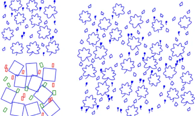
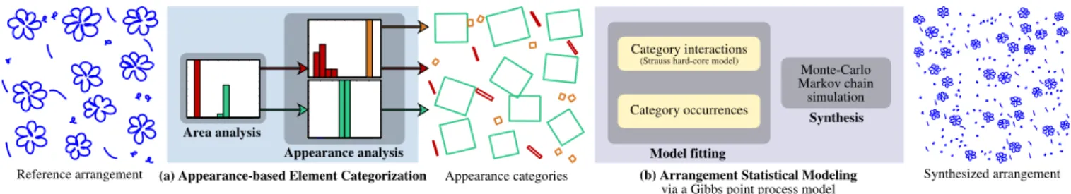
We use a physically-based fracture sim- ulation to generate new patterns, and we attempt to achieve visual similarity by matching appropriate statistics as deter- mined by the

In the case of Garside monoids, the main benefit of considering categories is that it allows for relaxing the existence of the global Garside element ∆ into a weaker, local

References

ASHIKHMIN, M. 2001. Synthesizing natural textures. I3D ’01, 217–226.
BARLA, P., BRESLAV, S., MARKOSIAN, L.,ANDTHOLLOT, J. 2006. Interactive hatching and stippling by example. Tech. rep., INRIA.
BARLA, P., BRESLAV, S., THOLLOT, J., SILLION, F.,ANDMARKOSIAN, L. 2006. Stroke Pattern Analysis and Synthesis. EUROGRAPHICS ’06 25, 3, 663–671. BESAG, J. 1977. Some methods of statistical analysis for spatial data. Bulletin of the
International Statistical Institute 47, 2, 77–92.
BILLIOT, J.-M., COEURJOLLY, J.-F.,ANDDROUILHET, R. 2008. Maximum pseu-dolikelihood estimator for exponential family models of marked gibbs point pro-cesses. Electronic Journal of Statistics 2, 234–264.
BRUNN, M., SOUSA, M. C.,ANDSAMAVATI, F. F. 2007. Capturing and re-using artistic styles with reverse subdivision-based multiresolution methods.
Interna-tional Journal of Image and Graphics ’07 7, 4, 593–615.
DESOLNEUX, A., MOISAN, L.,ANDMOREL, J.-M. 2000. Meaningful alignments.
International Journal of Computer Vision 40, 7–23.
DESOLNEUX, A., MOISAN, L.,ANDMORE, J. 2003. A grouping principle and four applications. IEEE Transactions on Pattern Analysis and Machine Intelligence 25, 4, 508–513.
DISCHLER, J.-M., MARITAUD, K., L ´EVY, B.,ANDGHAZANFARPOUR, D. 2002. Texture particles. EUROGRAPHICS ’02 21, 401–410.
EFROS, A. A.,ANDLEUNG, T. K. 1999. Texture synthesis by non-parametric sam-pling. ICCV ’99, 1033–1038.
FREEMAN, W. T., TENENBAUM, J. B.,ANDPASZTOR, E. 2003. Learning style translation for the lines of a drawing. ACM Transactions on Graphics 22, 1, 33–46. GEYER, C.,ANDMØLLER, J. 1994. Simulation procedures and likelihood inference
for spatial point processes. Scandinavian Journal of Statistics, 359–373. GREEN, P. J. 1995. Reversible jump Markov chain Monte Carlo computation and
Bayesian model determination. Biometrika 82, 4, 711–732.
GUO, G.-E., ZHU, S.-C.,ANDWU, Y. 2001. Visual learning by integrating descrip-tive and generadescrip-tive methods. ICCV ’01 1, 370–377.
HEEGER, D. J.,ANDBERGEN, J. R. 1995. Pyramid-based texture analysis/synthesis.
SIGGRAPH ’95, 229–238.
HERTZMANN, A., OLIVER, N., CURLESS, B.,ANDSEITZ, S. M. 2002. Curve analogies. Eurographics workshop on Rendering ’02, 233–246.
HUBERT, M., ROUSSEEUW, P.,ANDVERBOVEN, S. 2002. A fast method for ro-bust principal components with applications to chemometrics. Chemometrics and
Intelligent Laboratory Systems 60, 1-2, 101–111.
IJIRI, T., MECH, R., IGARASHI, T.,ANDMILLER, G. 2008. An Example-based Procedural System for Element Arrangement. EUROGRAPHICS ’08 27, 2, 429– 436.
JENSEN, J.,ANDMØLLER, J. 1991. Pseudolikelihood for exponential family models of spatial point processes. Annals of Applied Probability 1, 445–461.
JODOIN, P.-M., EPSTEIN, E., GRANGER-PICHE´, M.,ANDOSTROMOUKHOV, V. 2002. Hatching by example: a statistical approach. NPAR ’02, 29–36.
JULESZ, B. 1986. Texton gradients: The texton theory revisited. Biological
Cyber-netics 54, 4, 245–251.
KALNINS, R. D., MARKOSIAN, L., MEIER, B. J., KOWALSKI, M. A., LEE, J. C., DAVIDSON, P. L., WEBB, M., HUGHES, J. F.,ANDFINKELSTEIN, A. 2002. Wysiwyg npr: Drawing strokes directly on 3d models. SIGGRAPH ’02, 755–762. LEFEBVRE, S.,ANDHOPPE, H. 2006. Appearance-space texture synthesis.
SIG-GRAPH ’06 25, 541–548.
LIU, Y., COLLINS, R. T.,ANDTSIN, Y. 2004. A computational model for periodic pattern perception based on frieze and wallpaper groups. IEEE Transactions on
Pattern Analysis and Machine Intelligence 26, 354–371.
LIU, Y., LIN, W.-C.,ANDHAYS, J. 2004. Near-regular texture analysis and manip-ulation. SIGGRAPH ’04 23, 368–376.
RIPLEY, B. D. 1981. Spatial statistics. Wiley New York.
WEI, L.-Y.,ANDLEVOY, M. 2000. Fast texture synthesis using tree-structured vector quantization. SIGGRAPH ’00, 479–488.
WU, Q.,ANDYU, Y. 2004. Feature matching and deformation for texture synthesis.
SIGGRAPH ’04 23, 364–367.
Figure
Figure 1: Given a reference arrangement composed of vector elements (top left), our analysis scheme divides the raw element set into appearance categories (bottom left)
Figure 2: Overview of our method. First, our appearance-based element categorization (a) examines the reference elements’ shape and divides input elements into appearance categories
Figure 5: Synthesis results attesting the variety of spatial distributions that our model can handle
Figure 7: Example of user-drawn brush strokes whose intensity grants effective control over the synthesized densities of elements.
+2
Références
Documents relatifs