Rational homotopy -- Sullivan models
Texte intégral
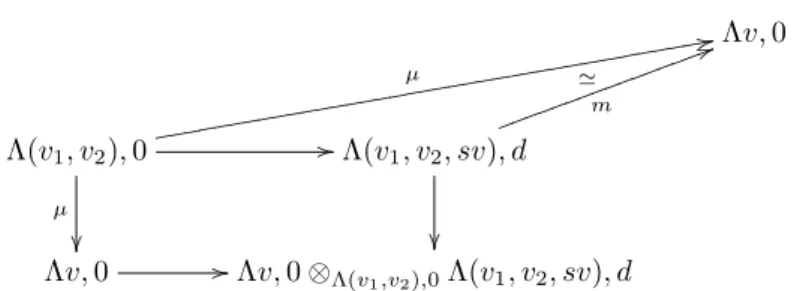
Figure
Documents relatifs
In order to achieve this, we represent L ( X ) as an ind-pro-object in the category of schemes of finite type and then show that the shifted de Rham complexes of the terms of
More recently, the second author classified in [Z] all holomorphic line bundles on LP1 that are invariant under a certain group of holomorphic automorphisms of L P I - -
When active learning (AL) is applied to help the user develop a model on a large dataset through interactively presenting data instances for labeling, existing AL techniques can
L’archive ouverte pluridisciplinaire HAL, est destinée au dépôt et à la diffusion de documents scientifiques de niveau recherche, publiés ou non, émanant des
Derek Sullivan, The Booklover Collection (detail), 2017, various artist publications, inkjet on paper, antique library tables Courtesy of the artist and Susan Hobbs Gallery,
Les tableaux de Sullivan sont des immensités flottantes qui semblent défier les lois de la gravité. Lorsque plusieurs sont présents ensemble dans l’atelier, ils
Ses travaux ont eu de nombreuses répercussions en psychiatrie alors qu'en psychanalyse la tendance est de considérer que Sullivan s'est suffisamment éloigné de
Dans la tradition de Locke et un peu à l'exemple du béhaviorisme, Sullivan s'est appliqué à démontrer combien les expériences relationnelles et culturelles déterminaient la
