Pépite | Impact des aérosols sur les nuages en Arctique

Texte intégral

(1)Thèse de Quentin Coopman, Lille 1, 2016. Numéro d’ordre : 42272. Université de Lille Sciences et Technologies École doctorale N◦ 104 : Sciences de la Matière, du Rayonnement et de l’Environnement Unité de recherche Laboratoire d’Optique Atmosphérique. Thèse présentée par Quentin Coopman Soutenue le 7 décembre 2016 En vue de l’obtention du grade de docteur de l’Université de Lille. Discipline Optique et Lasers, Physico-Chimie de l’Atmosphère. Impact des aérosols sur les nuages en Arctique Modification of arctic clouds by long-range aerosol transport. Thèse dirigée par. Jérôme RIEDI Timothy J. GARRETT. directeur co-directeur. Composition du jury Rapporteurs. Tristan S. L’ECUYER Kathy S. LAW. Examinateurs. Isabelle CHIAPELLO John C. LIN Gerald G. MACE Denis PETITPREZ. Université du Wisconsin LATMOS (Université Pierre et Marie Curie) LOA (Université de Lille) Université de l’Utah Université de l’Utah PC2A (Université de Lille). Jérôme RIEDI Timothy J. GARRETT. LOA (Université de Lille) Université de l’Utah. Directeurs de thèse. © 2016 Tous droits réservés.. président du jury. lilliad.univ-lille.fr.

(2) Thèse de Quentin Coopman, Lille 1, 2016. ABSTRACT The Arctic region is warming particularly rapidly. Aerosol impacts on cloud microphysical parameters are still poorly understood. Aerosol-cloud interactions (ACI) play an important role for cloud radiative properties and climate change. A challenge in the study of ACI is the use of independent datasets for cloud microphysical parameters and aerosol content so they cannot influence one another. In this study, we combine measurements from satellite instruments POLDER-3 and MODIS to temporally and spatially co-localate cloud microphysical properties with carbon monoxide concentrations from GEOS-Chem and FLEXPART, serving as a passive tracer of aerosol content. We also add ERA-I reanalysis of meteorological parameters to stratify meteorological parameters such as specific humidity and lower tropospheric stability. Thus, observed differences in cloud microphysical parameters can be attributed to differences in aerosol content rather than meteorological variability. We define a net Aerosol-Cloud Interaction parameter (ACInet ) which can be interpreted as a measure of the sensitivity of a cloud at any given location to pollution plumes from distant sources. We use this parameter to study the impact of aerosols from anthropogenic and biomass burning sources from mid-latitudes on liquid-cloud microphysical properties in Arctic, for a time period between 2005 and 2010, above ocean, and for controlled meteorological regimes. Our results suggest that the effect of biomass pollution plumes on clouds is smaller (ACInet ∼ 0) than that for anthropogenic pollution plumes (ACInet ∼. 0.30). Meteorological parameters can inhibit the aerosol-cloud interaction or favor the aerosol-cloud interaction. The impact of anthropogenic aerosol on thermodynamic phase transition are analyzed. The smaller the effective radius, the higher the supercooling temperature whereas the greater the aerosol concentration, the lower the supercooling temperature. Independently of changes in effective radius, decrease in energy barrier due to an increase in aerosol concentration can be up to 48%.. © 2016 Tous droits réservés.. lilliad.univ-lille.fr.

(3) Thèse de Quentin Coopman, Lille 1, 2016. ´ RESUM E´ Les interactions des aérosols avec les nuages en Arctique peuvent avoir de fortes conséquences sur le forçage radiatif des nuages. Néanmoins ces interactions restent encore mal comprises ou quantifiées . L’un des challenges de l’étude sur l’interaction aérosol-nuage est l’utilisation de jeux de données indépendant pour s’assurer qu’ils ne s’influencent pas mutuellement. Dans cette e´ tude nous utilisons les instruments satellitaires POLDER-3 & MODIS pour obtenir des informations sur les propriétés microphysiques des nuages que nous co-localisons temporellement et spatialement avec la concentration en monoxyde de carbone, traceur passif du contenu en aérosols, issue des modèles numriques GEOS-Chem et FLEXPART. Nous co-localisons e´ galement les données avec les réanalyses de ERA-Interim pour pouˆ voir controler les paramètres météorologiques tel que l’humidité spécifique et la stabilité de la basse troposphère. Afin d’étudier l’impact des panaches de pollution sur la microphysique des nuages, nous définissons le paramètre ACInet qui décrit l’interaction aérosol nuage. Nos résultats suggèrent que les parcelles d’air venant de feux de biomasses ont un effet limité sur la microphysique des nuages (ACInet ∼0). Au contraire, l’effet des aérosols venant de sources. anthropiques ont un effet proche du maximum théorique (ACInet ∼0,33). Nous avons alors e´ tudié l’impact de différent paramètres météorologiques sur l’ACInet .. Nous avons e´ galement analysé l’impact des aérosols d’origine anthropique sur la transition de phase liquide-glace des nuages. Nos résultats indiquent que le contenu en aérosols a un effet net de diminution de la température de transition de phase, ce qui est susceptible d’avoir de fortes conséquences sur la durée de vie des nuages. Indépendament des changements sur le rayon effectif des goutelettes d’eau, le changement de concentration en aérosols peut entraˆıner une diminution de la barrière e´ nergétique jusque 48%. Beaucoup d’études ont e´ té faites sur l’interaction aérosol-nuage, mais ce travail de thèse, basé sur la région Arctique, est original par l’utilisation de 6 ans de données satel-. © 2016 Tous droits réservés.. lilliad.univ-lille.fr.

(4) Thèse de Quentin Coopman, Lille 1, 2016. litaires, pour représenter les propriétés nuageuses, couplées a` des modèles numériques pour représenter le contenu en aérosols.. iii. © 2016 Tous droits réservés.. lilliad.univ-lille.fr.

(5) Thèse de Quentin Coopman, Lille 1, 2016. CONTENTS ABSTRACT . . . . . . . . . . . . . . . . . . . . . . . . . . . . . . . . . . . . . . . . . . . . . . . . . . . . . . . . . . . . .. i. ´ RESUM E´ . . . . . . . . . . . . . . . . . . . . . . . . . . . . . . . . . . . . . . . . . . . . . . . . . . . . . . . . . . . . . . .. ii. LIST OF FIGURES . . . . . . . . . . . . . . . . . . . . . . . . . . . . . . . . . . . . . . . . . . . . . . . . . . . . . . . vii LIST OF TABLES . . . . . . . . . . . . . . . . . . . . . . . . . . . . . . . . . . . . . . . . . . . . . . . . . . . . . . . . xiii ACKNOWLEDGEMENTS . . . . . . . . . . . . . . . . . . . . . . . . . . . . . . . . . . . . . . . . . . . . . . . . xv CHAPTERS 1.. 2.. GENERAL INTRODUCTION . . . . . . . . . . . . . . . . . . . . . . . . . . . . . . . . . . . . . . . . . .. 1. 1.1 Context . . . . . . . . . . . . . . . . . . . . . . . . . . . . . . . . . . . . . . . . . . . . . . . . . . . . . . . . . 1.1.1 Scientific context . . . . . . . . . . . . . . . . . . . . . . . . . . . . . . . . . . . . . . . . . . . . . 1.1.2 Arctic amplification . . . . . . . . . . . . . . . . . . . . . . . . . . . . . . . . . . . . . . . . . . . 1.1.3 Future arctic climate . . . . . . . . . . . . . . . . . . . . . . . . . . . . . . . . . . . . . . . . . . 1.1.4 Cloud and sea-ice feedbacks . . . . . . . . . . . . . . . . . . . . . . . . . . . . . . . . . . . . 1.2 Clouds and their role in the climate system . . . . . . . . . . . . . . . . . . . . . . . . . . . . 1.2.1 Cloud formation . . . . . . . . . . . . . . . . . . . . . . . . . . . . . . . . . . . . . . . . . . . . . . 1.2.2 Cloud extinction of radiation . . . . . . . . . . . . . . . . . . . . . . . . . . . . . . . . . . . 1.2.3 Cloud-droplet effective radius . . . . . . . . . . . . . . . . . . . . . . . . . . . . . . . . . . 1.2.4 Liquid water path . . . . . . . . . . . . . . . . . . . . . . . . . . . . . . . . . . . . . . . . . . . . 1.2.5 Cloud radiative properties and cloud radiative forcing . . . . . . . . . . . . . . 1.2.6 Cloud radiative impacts in the Arctic . . . . . . . . . . . . . . . . . . . . . . . . . . . . . 1.3 Aerosols in the Arctic . . . . . . . . . . . . . . . . . . . . . . . . . . . . . . . . . . . . . . . . . . . . . . 1.4 Impact of aerosols on liquid-cloud microphysical properties . . . . . . . . . . . . . . 1.4.1 The Aerosol-cloud parameter . . . . . . . . . . . . . . . . . . . . . . . . . . . . . . . . . . . 1.4.2 Aerosol-cloud interaction from different methods . . . . . . . . . . . . . . . . . . 1.4.3 Aerosol-cloud interactions from satellite and models . . . . . . . . . . . . . . . . 1.4.4 Impact of aerosols on liquid-cloud radiative forcing . . . . . . . . . . . . . . . . 1.5 Impact of aerosols on ice-cloud microphysical properties . . . . . . . . . . . . . . . . . 1.5.1 Nature of ice nuclei . . . . . . . . . . . . . . . . . . . . . . . . . . . . . . . . . . . . . . . . . . . 1.5.2 Modes of action . . . . . . . . . . . . . . . . . . . . . . . . . . . . . . . . . . . . . . . . . . . . . . 1.5.3 Theory of heterogeneous nucleation . . . . . . . . . . . . . . . . . . . . . . . . . . . . . 1.6 Influence of meteorological parameters on cloud microphysical parameters . 1.7 Summary of dissertation . . . . . . . . . . . . . . . . . . . . . . . . . . . . . . . . . . . . . . . . . . .. 1 1 3 5 7 8 8 9 10 11 11 14 15 17 19 20 24 26 26 27 28 28 30 33. INSTRUMENTS, MODEL, REANALYSIS AND DATASET . . . . . . . . . . . . . . . . . 35 2.1 Cloud parameters from satellite instruments . . . . . . . . . . . . . . . . . . . . . . . . . . . 35 2.1.1 The POLDER/PARASOL Mission . . . . . . . . . . . . . . . . . . . . . . . . . . . . . . . 35 2.1.2 MODIS . . . . . . . . . . . . . . . . . . . . . . . . . . . . . . . . . . . . . . . . . . . . . . . . . . . . . 36. © 2016 Tous droits réservés.. lilliad.univ-lille.fr.

(6) Thèse de Quentin Coopman, Lille 1, 2016. 2.1.3 Parameters used in this study . . . . . . . . . . . . . . . . . . . . . . . . . . . . . . . . . . . 2.2 Passive tracer from numerical tracer transport models . . . . . . . . . . . . . . . . . . . 2.2.1 CO as a passive tracer of aerosols . . . . . . . . . . . . . . . . . . . . . . . . . . . . . . . . 2.2.2 FLEXPART . . . . . . . . . . . . . . . . . . . . . . . . . . . . . . . . . . . . . . . . . . . . . . . . . . 2.2.3 GEOS-Chem . . . . . . . . . . . . . . . . . . . . . . . . . . . . . . . . . . . . . . . . . . . . . . . . . 2.3 Meteorological parameters from ERA-Interim datasets . . . . . . . . . . . . . . . . . . 2.4 Co-location of multiple datasets . . . . . . . . . . . . . . . . . . . . . . . . . . . . . . . . . . . . . 3.. TEMPORAL AND GEOGRAPHICAL VARIABILITY OF PARAMETERS . . . . . 52 3.1 Cloud properties . . . . . . . . . . . . . . . . . . . . . . . . . . . . . . . . . . . . . . . . . . . . . . . . . . 3.1.1 Cloud Phase . . . . . . . . . . . . . . . . . . . . . . . . . . . . . . . . . . . . . . . . . . . . . . . . . 3.1.2 Liquid cloud optical depth . . . . . . . . . . . . . . . . . . . . . . . . . . . . . . . . . . . . . 3.1.3 Liquid cloud droplet effective radius . . . . . . . . . . . . . . . . . . . . . . . . . . . . . 3.1.4 Uncertainty on Liquid cloud droplet effective radius . . . . . . . . . . . . . . . . 3.1.5 Cloud top height . . . . . . . . . . . . . . . . . . . . . . . . . . . . . . . . . . . . . . . . . . . . . 3.2 Pollution concentrations . . . . . . . . . . . . . . . . . . . . . . . . . . . . . . . . . . . . . . . . . . . 3.2.1 Temporal variations of CO concentration . . . . . . . . . . . . . . . . . . . . . . . . . 3.2.2 Geographical variation . . . . . . . . . . . . . . . . . . . . . . . . . . . . . . . . . . . . . . . . 3.3 Meteorological parameters of the Arctic . . . . . . . . . . . . . . . . . . . . . . . . . . . . . . . 3.3.1 Winds . . . . . . . . . . . . . . . . . . . . . . . . . . . . . . . . . . . . . . . . . . . . . . . . . . . . . . 3.3.2 Specific humidity . . . . . . . . . . . . . . . . . . . . . . . . . . . . . . . . . . . . . . . . . . . . . 3.3.3 Lower tropospheric stability . . . . . . . . . . . . . . . . . . . . . . . . . . . . . . . . . . . . 3.3.4 Monthly variability coincident with liquid cloud . . . . . . . . . . . . . . . . . . .. 4.. 52 53 53 53 59 59 62 64 67 69 69 70 71 73. EFFECT OF LONG-RANGE AEROSOL TRANSPORT ON THE MICROPHYSICAL PROPERTIES OF LOW-LEVEL LIQUID CLOUDS IN THE ARCTIC . . . . . . . . . 75 4.1 Introduction . . . . . . . . . . . . . . . . . . . . . . . . . . . . . . . . . . . . . . . . . . . . . . . . . . . . . 4.2 Data . . . . . . . . . . . . . . . . . . . . . . . . . . . . . . . . . . . . . . . . . . . . . . . . . . . . . . . . . . . . 4.3 Methodology . . . . . . . . . . . . . . . . . . . . . . . . . . . . . . . . . . . . . . . . . . . . . . . . . . . . . 4.3.1 Co-location of satellite retrieval and model pollution tracer fields . . . . . 4.3.2 The net aerosol-cloud interactions parameter . . . . . . . . . . . . . . . . . . . . . . 4.3.3 Stratifying the data for specific humidity and lower tropospheric stability . . . . . . . . . . . . . . . . . . . . . . . . . . . . . . . . . . . . . . . . . . . . . . . . . . . . . . . 4.4 Results . . . . . . . . . . . . . . . . . . . . . . . . . . . . . . . . . . . . . . . . . . . . . . . . . . . . . . . . . . 4.4.1 Net Aerosol-Cloud Interactions . . . . . . . . . . . . . . . . . . . . . . . . . . . . . . . . . 4.4.2 Dependence of ACInet on pollution concentration, specific humidity, and lower tropospheric stability . . . . . . . . . . . . . . . . . . . . . . . . . . . . . . . . . 4.5 Discussion . . . . . . . . . . . . . . . . . . . . . . . . . . . . . . . . . . . . . . . . . . . . . . . . . . . . . . . 4.6 Conclusion . . . . . . . . . . . . . . . . . . . . . . . . . . . . . . . . . . . . . . . . . . . . . . . . . . . . . .. 5.. 39 41 41 41 42 48 49. 76 79 79 79 80 82 84 84 86 89 92. IMPACT OF ANTHROPOGENIC AND BIOMASS BURNING PLUMES ON ARCTIC CLOUDS . . . . . . . . . . . . . . . . . . . . . . . . . . . . . . . . . . . . . . . . . . . . . . . . . . . 94 5.1 5.2 5.3 5.4 5.5. Introduction . . . . . . . . . . . . . . . . . . . . . . . . . . . . . . . . . . . . . . . . . . . . . . . . . . . . . ACInet parameter . . . . . . . . . . . . . . . . . . . . . . . . . . . . . . . . . . . . . . . . . . . . . . . . . Data used . . . . . . . . . . . . . . . . . . . . . . . . . . . . . . . . . . . . . . . . . . . . . . . . . . . . . . . Case study of 31 July 2010 . . . . . . . . . . . . . . . . . . . . . . . . . . . . . . . . . . . . . . . . . . Results and discussion . . . . . . . . . . . . . . . . . . . . . . . . . . . . . . . . . . . . . . . . . . . . .. 95 95 96 96 97. v. © 2016 Tous droits réservés.. lilliad.univ-lille.fr.

(7) Thèse de Quentin Coopman, Lille 1, 2016. 5.6 Conclusion . . . . . . . . . . . . . . . . . . . . . . . . . . . . . . . . . . . . . . . . . . . . . . . . . . . . . . 101 6.. IMPACT OF ANTHROPOGENIC POLLUTION PLUMES ON THERMODYNAMIC PHASE TRANSITION . . . . . . . . . . . . . . . . . . . . . . . . . . . . . . . . . . . . . . . . . . . . . . . . 103 6.1 6.2 6.3 6.4. 7.. Introduction . . . . . . . . . . . . . . . . . . . . . . . . . . . . . . . . . . . . . . . . . . . . . . . . . . . . . 103 Data . . . . . . . . . . . . . . . . . . . . . . . . . . . . . . . . . . . . . . . . . . . . . . . . . . . . . . . . . . . . 105 Results & Discussions . . . . . . . . . . . . . . . . . . . . . . . . . . . . . . . . . . . . . . . . . . . . . . 106 Conclusion . . . . . . . . . . . . . . . . . . . . . . . . . . . . . . . . . . . . . . . . . . . . . . . . . . . . . . 112. SUMMARY AND FUTURE WORK . . . . . . . . . . . . . . . . . . . . . . . . . . . . . . . . . . . . . 114 7.1 General Conclusions . . . . . . . . . . . . . . . . . . . . . . . . . . . . . . . . . . . . . . . . . . . . . . . 114 7.2 Future works . . . . . . . . . . . . . . . . . . . . . . . . . . . . . . . . . . . . . . . . . . . . . . . . . . . . . 117. APPENDIX: SEA ICE EXTENT . . . . . . . . . . . . . . . . . . . . . . . . . . . . . . . . . . . . . . . . . . . . . 121 REFERENCES . . . . . . . . . . . . . . . . . . . . . . . . . . . . . . . . . . . . . . . . . . . . . . . . . . . . . . . . . . . 124. vi. © 2016 Tous droits réservés.. lilliad.univ-lille.fr.

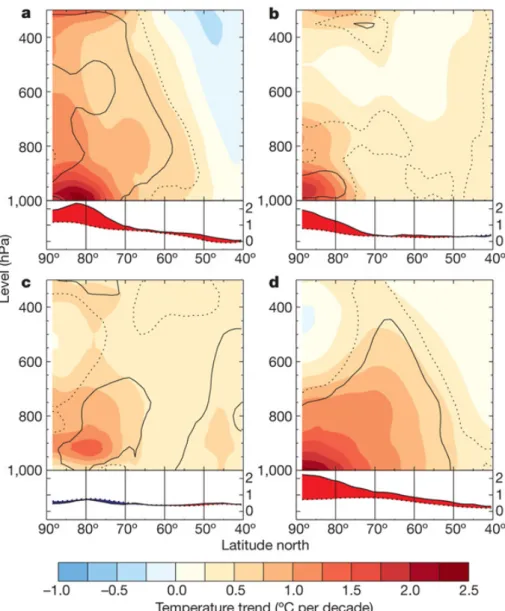
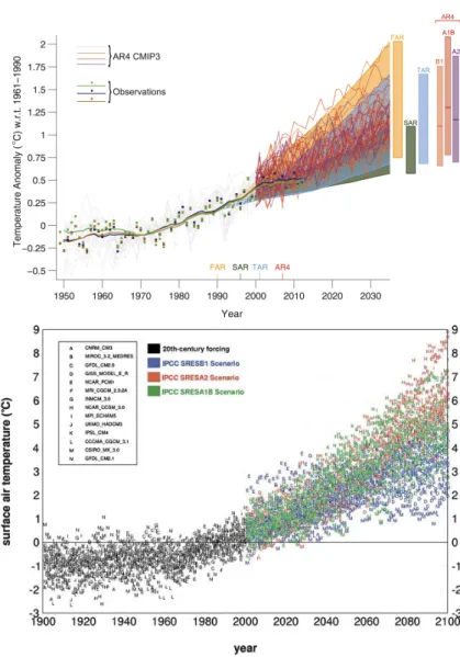
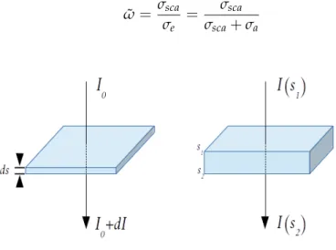
(8) Thèse de Quentin Coopman, Lille 1, 2016. LIST OF FIGURES. 1.1. 1.2. 1.3. © 2016 Tous droits réservés.. Zonal average of temperature trends for winter (December to February; a), spring (March to May; b), summer (June to August; c) and autumn (September to November; d). The black outlines indicate where trends differ significantly from zero at the 99% (solid lines) and 95% (dotted lines) confidence levels. The line graphs show trends (same units as in color plots) averaged over the lower part of the atmosphere (950-1,000 hPa; solid lines) and over the entire atmospheric column (300-1,000 hPa; dotted lines). Red shading indicates that the lower atmosphere has warmed faster than the atmospheric column as a whole. Blue shading indicates that the lower atmosphere has warmed slower than the atmospheric column as a whole (Screen and Simmonds, 2010). . . . . . . . . . . . . . . . . . . . . . . . . . . . . . . . . . . . . . . . . . . . . . . . . . . . . . .. 4. top: Estimated changes in the observed globally and annually averaged surface temperature anomaly relative to 1961-1990 (in ◦ C) since 1950 was compared with the range of projections from the previous IPCC assessments. Values are harmonized to start from the same value as in 1990. Observed global annual mean surface air temperature anomaly, relative to 1961-1990, is shown as squares and smoothed time series as solid lines (National Aeronautics and Space Administration (NASA) (dark blue), National Oceanic and Atmospheric Administration (NOAA) (warm mustard), and the UK Hadley Centre (bright green) reanalyses). The colored shading shows the projected range of the global annual mean surface air temperature change from 1990 to 2035 for models used in FAR, SAR, TAR. TAR results are based on the simple climate model analyses presented and not on the individual full three-dimensional climate model simulations. For the AR4, results are presented as single model runs of the CMIP3 ensemble for the historical period from 1950 to 2000 (light grey lines) and for three scenarios (A2, A1B and B1) from 2001 to 2035. The bars at the right-hand side of the graph show the full range given for 2035 for each assessment report. (IPCC, 2013). bottom: Simulated and projected annual mean arctic surface air temperature, expressed as departures from 1981-2000 means, by 14 global climate models for the twentieth- and twentyfirst centuries. Projections use three greenhouse gas forcing scenarios: IPCC SRESB1 (blue), IPCC SRESA1B (green), and IPCC SRESA2 (red) (Chapman and Walsh, 2007a) . . . . . . . . . . . . . . . . . . . . . . . . . . . . . . . . . . . . . . . . . . . . . . . . . .. 6. Left: An incoming radiation with intensity I0 goes through a layer with a thickness ds. The radiation exits the layer with a change in intensity of dI. Right: The layer is not infinitesimal, the incoming radiation with intensity I (s1 ) exits the layer with an intensity I (s2 ). . . . . . . . . . . . . . . . . . . . . . . . . . . . . .. 9. lilliad.univ-lille.fr.

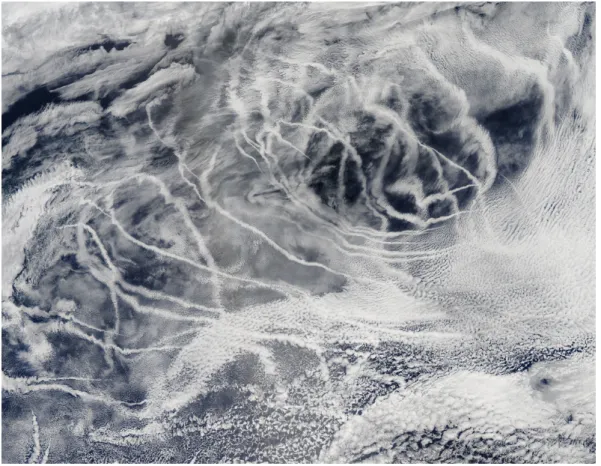
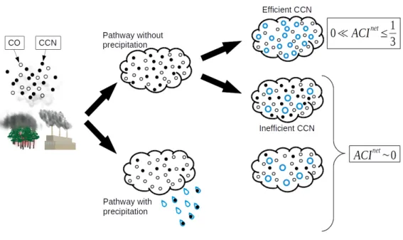
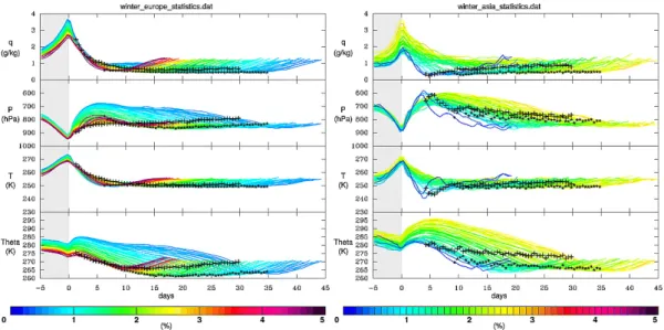
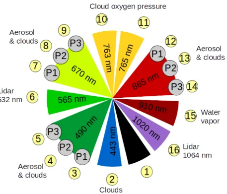
(9) Thèse de Quentin Coopman, Lille 1, 2016. 1.4. Schematic showing of pathways for the transport of air pollution into the Arctic. Following Stohl (2006), three main routes are evident: 1) low-level transport from mid-latitude emission regions followed by uplift at the arctic front; 2) lifting of pollutants at lower latitudes, followed by upper tropospheric transport and possible slow descent (due to radiative cooling) or mixing into the polar dome — a frequent transport route from North America and Asia, but prone to significant wet scavenging; and 3) wintertime lowlevel transport of already cold air into the polar dome, mainly from northern Eurasia. Emissions from strong boreal fires could be lifted by pyroconvection (Fromm, 2005) and later entrained into the polar dome (Law et al., 2014). . . . . . 17. 1.5. Satellite picture acquired on July 3, 2010 by MODIS (Moderate-Resolution Imaging Spectroradiometer) in the North Pacific (from NASA’s Earth Observatory). . . . . . . . . . . . . . . . . . . . . . . . . . . . . . . . . . . . . . . . . . . . . . . . . . . . . . . . . . . . 18. 1.6. Relation between CO concentration and aerosol concentration along different pathways. . . . . . . . . . . . . . . . . . . . . . . . . . . . . . . . . . . . . . . . . . . . . . . . . . . . . . . . . . 25. 1.7. Seasonally mean change in arctic liquid-cloud shortwave radiative forcing (∆CRFSW in blue) and arctic liquid-cloud longwave radiative forcing (∆CRFSW in red) associated with haze pollution in Barrow (Alaska). Data are from Table 1 in Zhao and Garrett (2015). . . . . . . . . . . . . . . . . . . . . . . . . . . . . . . . . . . . . 27. 1.8. Free Gibbs energy (blue), volume free energy (green), and interfacial energy (red) of a germ of a cluster for homogeneous nucleation as function of the radius of the cluster. . . . . . . . . . . . . . . . . . . . . . . . . . . . . . . . . . . . . . . . . . . . . . . . . 29. 1.9. Left: Meteorological parameters (top plot, q; second plot, p; third plot, T; bottom plot, Q) along trajectories from the European box to the arctic lower troposphere. Every line represents an average over one of 60 transport time bins from half a day to 30 days, and its color shows the relative frequency of such cases. Days -5 to 0 (gray shaded) are the period before particles left the source region, the time when they entered the Arctic is marked with a plus, and 5 days later an asterisk is drawn. Right: Same as left panel, but for trajectories from the Asian box (Stohl, 2006) . . . . . . . . . . . . . . . . . . . . . . . . . . . . . 32. 2.1. The A-train constellation. As od December 2013, PARASOL stopped recording data and OCO failed during the launch, but OCO-2 is now in orbit (NASA’s Earth Observatory). . . . . . . . . . . . . . . . . . . . . . . . . . . . . . . . . . . . . . . . . . . . . . . . . . 36. 2.2. The different spectral channels of POLDER-3. P1 (+60◦ ), P2(0◦ ), and P3 (-60◦ ) represent the 3 polarized directions of the filters (CNES). . . . . . . . . . . . . . . . . . . 37. 2.3. Weight attributed to POLDER and MODIS cloud top pressure when the cloudtop-pressure measurements are between 600 and 800 hPa. . . . . . . . . . . . . . . . . . 40. 2.4. Normalized cloud thermodynamic phase index frequency distribution from the POLDER-MODIS algorithm, for pixels with the phase-index SD less than 10. Colors represent different cloud altitudes, between 200–1000 m in red and between 1000–2000 m in black. . . . . . . . . . . . . . . . . . . . . . . . . . . . . . . . . . . . . . . . . 40 viii. © 2016 Tous droits réservés.. lilliad.univ-lille.fr.

(10) Thèse de Quentin Coopman, Lille 1, 2016. 2.5. Source regions for the tagged CO simulation. Regions outlined in red denote fossil fuel tagged tracers; regions outlined in green refer to biomass-burning tagged tracers. . . . . . . . . . . . . . . . . . . . . . . . . . . . . . . . . . . . . . . . . . . . . . . . . . . . . . 44. 2.6. Stations, from the NOAA ESRL network, from which the CO-concentration flask measurements are compared with modeled CO. . . . . . . . . . . . . . . . . . . . . . 45. 2.7. 2D distribution and linear regression of GEOS-Chem total CO concentration as function of CO-concentration observation from flask measurement from 5 different arctic stations between 2005 and 2010. Value of correlation coefficient (r), the p-value, the standard error, and the number of measurements are shown. . . . . . . . . . . . . . . . . . . . . . . . . . . . . . . . . . . . . . . . . . . . . . . . . . . . . . . . . 46. 2.8. Time series of total CO concentration between 2005 and 2010 from GEOSChem (gray lines) with the associated total CO-concentration flask measurements (blue points) from NOAA ESRL from 5 arctic stations. . . . . . . . . . . . . . . . 47. 2.9. Illustration of the horizontal co-location method, showing satellite data corresponding to cloud top pressures below 1000 m altitude (gray shading), the average FLEXPART CO concentration between 1 and 2 km (colored shading), and the spatial resolution of temperature profiles and SH in blue points. The black grid, at the top of the map, corresponds to the sinusoidal equal-area grid used in this study for co-locating each data set. . . . . . . . . . . . . . . . . . . . . . . 51. 3.1. Monthly frequency of liquid clouds referring to low-level clouds over the Arctic from MODIS and POLDER instrument from April 2005 to September 2010 for a layer between 700 and 1,013 hPa. . . . . . . . . . . . . . . . . . . . . . . . . . . . . . 54. 3.2. Monthly frequency of ice clouds referring to low-level clouds over the Arctic from MODIS and POLDER instrument from April 2005 to September 2010 for a layer between 700 and 1,013 hPa. . . . . . . . . . . . . . . . . . . . . . . . . . . . . . . . . . 55. 3.3. Stereographic projections of the seasonal occurrence of: (a) all clouds (referring to time) and (b) MPCs (referring to clouds). Occurrences are computed taking into account the 500 to 12,000 m altitude range (Mioche et al., 2014). . . . 56. 3.4. Monthly liquid cloud optical depth over the Arctic from MODIS instrument from April 2005 to September 2010 for a layer between 700 and 1,013 hPa. . . . . 57. 3.5. same as Fig. 3.4 but considering the liquid-cloud-droplet effective radius. . . . . 58. 3.6. Monthly liquid cloud effective radius uncertainty over the Arctic from MODIS instrument from April 2005 to September 2010 for a layer between 700 and 1,013 hPa. . . . . . . . . . . . . . . . . . . . . . . . . . . . . . . . . . . . . . . . . . . . . . . . . . . . . . . . . . 60. 3.7. Normalized distributions of liquid and ice-cloud heights for different seasons from March 2005 to September 2010 above the arctic circle from POLDER-3 cloud top height. . . . . . . . . . . . . . . . . . . . . . . . . . . . . . . . . . . . . . . . . . . . . . . . . . . . 61. 3.8. Map of the seasonally average of the CO concentration between 975 and 800 hPa and between 2005 and 2010 from GEOS-Chem. On the left, maps represent the anthropogenic CO concentration, and on the right maps represent the biomass-burning CO concentration. . . . . . . . . . . . . . . . . . . . . . . . . . . . . 63 ix. © 2016 Tous droits réservés.. lilliad.univ-lille.fr.

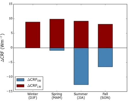
(11) Thèse de Quentin Coopman, Lille 1, 2016. 3.9. Pie charts of seasonal CO source regions from which pollution plumes reach the Arctic from GEOS-Chem model, considering fossil-fuel (top) and biomassburning (bottom) combustion out of total. . . . . . . . . . . . . . . . . . . . . . . . . . . . . . . 64. 3.10. Map of the monthly average of biomass burning fraction between 975 and 800 hPa and between 2005 and 2010 from GEOS-Chem. . . . . . . . . . . . . . . . . . . . 65. 3.11. Temporal distribution of the CO-concentration yearly averaged from 2005 to 2010 retrieved by GEOS-Chem for the arctic region (latitude greater than 65◦ ). We differentiate anthropogenic pollution plumes to biomass pollution by considering the biomass-burning concentration fraction. A fraction below 0.2 identifies anthropogenic pollution plumes and a fraction above 0.8 identifies a biomass-burning pollution plumes. Polluted and clean plumes are identified considering respectively the upper and lower quartile of CO concentration. . . . . . . . . . . . . . . . . . . . . . . . . . . . . . . . . . . . . . . . . . . . . . . . . . . . . . 66. 3.12. Geographical distribution of plumes by latitude. . . . . . . . . . . . . . . . . . . . . . . . . . 67. 3.13. Same as Fig. 3.11 considering the geographical distribution of longitudes. . . . . 68. 3.14. Map of seasonally averaged horizontal winds at 700 hPa between 2005 and 2010 from ERA-I displayed in wind barbs in knots. The pressure velocity at 700 hPa is also shown by the color scale. Winter is defined as JanuaryFebruary-March, spring is defined as April-Mai-June, summer as July-AugustSeptember, and fall as October, November, December. . . . . . . . . . . . . . . . . . . . . 70. 3.15. Map of seasonally averaged specific humidity at 700 hPa between 2005 and 2010 from ERA-I. Winter is defined as January-February-March, spring is defined as April-Mai-June, summer as July-August-September, and fall as October, November, December. . . . . . . . . . . . . . . . . . . . . . . . . . . . . . . . . . . . . . . . 71. 3.16. Same as Fig. 3.16 but for the lower tropospheric stability. . . . . . . . . . . . . . . . . . . 72. 3.17. 2D histogram of the specific humidity and the lower tropospheric stability between 2005 and 2010 coincident with liquid low-level clouds with latitudes greater than 65◦ . Each point is associated with the month when it is most likely to be retrieved. . . . . . . . . . . . . . . . . . . . . . . . . . . . . . . . . . . . . . . . . . . . . . . . 73. 4.1. Calculation of the ACInet re parameter from a probability distribution of values in the effective radius and CO tracer concentration for liquid clouds with cloud top altitudes between 1000 m and 2000 m, and cloud top temperatures between −12 and 6.0 ◦ C. The color scale indicates higher density of values in linear intervals. The ACInet re number indicates the negative slope of the linear fit (dashed line). . . . . . . . . . . . . . . . . . . . . . . . . . . . . . . . . . . . . . . . . . . . . . . . . . . . . 82. 4.2. 2-D histogram of the SH and the LTS retrieved by ECMWF reanalysis from 2008 to 2010. The red rectangle corresponds to the range where there is a maximum of measurements within a bin corresponding to 15 % of the total range length of the corresponding parameter. . . . . . . . . . . . . . . . . . . . . . . . . . . . 83 x. © 2016 Tous droits réservés.. lilliad.univ-lille.fr.

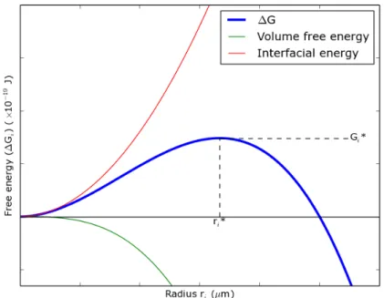
(12) Thèse de Quentin Coopman, Lille 1, 2016. 4.3. ACInet parameter of the effective radius (re ) (red) and optical depth (τ) (black), as a function of temperature calculated for liquid clouds between 200–1000 m (lower row) and 1000–2000 m (upper row). The bars indicate the 95 % confidence limit in the calculation of the mean ACInet value. Each column corresponds to different thresholds for LWP (blackbody: LWP > 40 g m−2 , graybody: LWP < 40 g m−2 ). Blue numbers indicate the number of grid-cells, in hundreds, that are used to calculate each ACInet value. In each figure the ACInet value averaged over the temperature and weighted according the inverse of the uncertainty is indicated. . . . . . . . . . . . . . . . . . . . . . . . . . . . . . . . . . 85. 4.4. ACIrnet (red) and ACInet τ (black) for different bins of the SH, stratified by LTS e between 17 and 22 K. Each marker is placed in the middle of the corresponding bin. . . . . . . . . . . . . . . . . . . . . . . . . . . . . . . . . . . . . . . . . . . . . . . . . . . . . . . . . . . . 88. 4.5. net net ACInet re (red) and ACIτ (black) and ACIτ as a function of the lower tropospheric stability, stratified by SH between 2.0 and 4.0 g kg−1 . . . . . . . . . . . . . . . . 88. 4.6. Normalized distribution of the cloud top potential temperature when clouds are associated with CO tracer concentrations (χCO ) greater than 10 ppbv and less than 5 ppbv. The values of ACIrnet and ACInet τ associated with each hise togram are presented also in Table 4.3. . . . . . . . . . . . . . . . . . . . . . . . . . . . . . . . . . 91. 5.1. Low-level τ, SH at 700 hPa and χCO of the first 3 km on 31 July at 21:30 UTC. The SH and the χCO are respectively retrieved by ERA-Interim reanalysis, and GEOS-Chem and they are both showing by the contour plots. Values of τ are retrieved by the instrument Aqua on MODIS platform satellite. . . . . . . . . 97. 5.2. Normalized probability density function of (a,d) SH, (b,e) LTS, and (c,f) TC for clean and polluted air parcels during (a,b,c) ANT and (d,e,f) BB aerosol regimes. Clean and polluted BB air parcels corresponding to the lower and upper quartiles in CO concentration have values of χCO less than 155 ppb and greater than 262 ppb, respectively. Clean and polluted ANT air parcels have values of χCO less than 54 ppb and greater than 82 ppb. . . . . . . . . . . . . . . . 99. 5.3. ACIrnet (a) as function of biomass burning fraction χCO ( BB)/χCO , LWP, and e (b) whether the dataset is limited to a narrow range of LTS and SH with TC between -7.8◦ C and 4.8◦ C. Error bars indicate 95% confidence ranges for the calculated value of ACI net . N indicates the number of equal-area grid cells containing clouds that went into the calculation of the ACI net parameter for the combined 4 LWP bins. ACIτnet - ACIrnet is shown only when the difference e between the two values is statistically significant (Methods). The light blue area bounded by the yellow line represents the difference between the ACIrnet e averaged over the 4 LWP bins and a theoretical maximum value of 0.33. Red and blue areas represent the calculated increase and decrease, respectively in ACIrnet that is due to controlling for meteorology. . . . . . . . . . . . . . . . . . . . . . . . . 100 e. 6.1. (a) Ice fraction as function of cloud top temperature for 4 χCO regimes defined by χCO distribution quartiles. (b) Hyperbolic tangential fit of the ice fraction as function of the cloud top temperature, for the 4 χCO regimes, presented by Equation (6.1). . . . . . . . . . . . . . . . . . . . . . . . . . . . . . . . . . . . . . . . . . . . . . . . . . . . . . 107 xi. © 2016 Tous droits réservés.. lilliad.univ-lille.fr.

(13) Thèse de Quentin Coopman, Lille 1, 2016. 6.2. Cloud repartition by the ISCCP as a function of the cloud top altitude and cloud optical depth. Boxes with a thicker border are the cloud types considered in this study. . . . . . . . . . . . . . . . . . . . . . . . . . . . . . . . . . . . . . . . . . . . . . . . . . . 108. 6.3. ∆T* as function of the liquid-cloud-droplet effective radius for 4 cloud categories differentiated by their optical depth and top pressure. . . . . . . . . . . . . . . . 109. 6.4. Parameters a1 (solid) and a2 (hollow), from Eq. (6.1), as function of the CO concentration (χCO ). Parameters a1 and a2 defined respectively the flatness and the shift of the hyperbolic tangential fit of the ice fraction versus the cloud top temperature. Results are presented for 4 cloud categories differentiated by their optical depth and top pressure. . . . . . . . . . . . . . . . . . . . . . . . . . . . . . . . . 110. 6.5. ∆T* as function of the CO concentration (χCO ) for 4 cloud categories differentiated by their optical depth and top pressure. The color scale corresponds to the associated mean liquid-cloud droplet effective radius. . . . . . . . . . . . . . . . 111. A.1. Average monthly sea-ice concentration, for the year from 2005 to 2010, defined as the fractional coverage normalized from January to June. We used the months in the years from 2005 to 2010. . . . . . . . . . . . . . . . . . . . . . . . . . . . . . . 122. A.2. Same as Fig. A.1 but from August to December. . . . . . . . . . . . . . . . . . . . . . . . . . . 123. xii. © 2016 Tous droits réservés.. lilliad.univ-lille.fr.

(14) Thèse de Quentin Coopman, Lille 1, 2016. LIST OF TABLES. © 2016 Tous droits réservés.. 1.1. Values from the literature quantifying the aerosol-cloud interaction using some variant of Eq. (1.25), are expressed here as ACI parameters. All values have been converted to the form, as in Eq. (1.25) for comparison purposes. All studies address low or liquid clouds . . . . . . . . . . . . . . . . . . . . . . . . . . . . . . . . 22. 1.1. Table 1.1 continued . . . . . . . . . . . . . . . . . . . . . . . . . . . . . . . . . . . . . . . . . . . . . . . . . 23. 2.1. Characteristics of spectral bands selected for the MODIS instrument aboard AQUA (Ackerman et al., 1998) . . . . . . . . . . . . . . . . . . . . . . . . . . . . . . . . . . . . . . . . 38. 2.2. Description of the 5 different stations, from NOAA ESRL, considered to compare χCO from GEOS-Chem and χCO from in-situ samples. Latitudes, longitudes, altitudes of the stations are shown with the associated GEOS-Chem vertical box. . . . . . . . . . . . . . . . . . . . . . . . . . . . . . . . . . . . . . . . . . . . . . . . . . . . . . . . 44. 2.3. Results of the linear regression of total CO concentration from GEOS-Chem as function of the total CO concentration from in-situ flask for five different arctic stations. From the linear fit the slope (α), the correlation coefficient (r), standard deviation (σ), the number of measurements, and the median of the difference between the two sets are shown. . . . . . . . . . . . . . . . . . . . . . . . . . . . . . 46. 4.1. Cloud products, pollution tracer, atmospheric reanalysis used in this study with the corresponding spatial and temporal resolution. . . . . . . . . . . . . . . . . . . 79. 4.2. Summary of the different ranges of the logarithm of the SH and the LTS over the region of interest, detailing the method used to determine the final range of parameters considered. The ∆ defines the difference between the maximum and the minimum of the total range. The considered range is chosen to keep the maximum number of measurements within a fixed interval of 15 % of the range, corresponding to the red square on Fig. 4.2. . . . . . . . . . . . . . . . . . . 83. 4.3. ACInet parameter calculated for the optical depth and the effective radius considering all clouds, graybody clouds and blackbody clouds, averaged from values presented in Fig. 4.3 and weighted considering the inverse of the uncertainty in the mean. . . . . . . . . . . . . . . . . . . . . . . . . . . . . . . . . . . . . . . . . . . 86. 4.4. ACInet parameter calculated for the optical depth and the effective radius considering all clouds, graybody clouds, and blackbody clouds, for two different regimes of CO concentration representing lower and upper quartiles of CO concentration. . . . . . . . . . . . . . . . . . . . . . . . . . . . . . . . . . . . . . . . . . . . . . . . . 87. 4.5. Percentile values of SH and LTS used to defined different regimes of the meteorological parameters. . . . . . . . . . . . . . . . . . . . . . . . . . . . . . . . . . . . . . . . . . . 87. lilliad.univ-lille.fr.

(15) Thèse de Quentin Coopman, Lille 1, 2016. 4.6. net net Difference between ACInet τ and ACIre (i.e. ACILWP ) for graybody, blackbody, and all clouds when lower tropospheric stability and SH are stratified and when they are not stratified. The averaged ACInet values are shown in Table 3. 90. 5.1. Meteorological parameters associated with ANT and BB aerosol regimes. Median values of the specific humidity (SH), the lower-tropospheric stability (LTS), and cloud-top temperature are associated with BB and ANT aerosol regimes and for all grid cells . . . . . . . . . . . . . . . . . . . . . . . . . . . . . . . . . . . . . . . . . 98. 6.1. Ratio of the free energy barrier of the thermodynamic phase transition between polluted and clean air pollution plumes is inferred from Fig. 6.5. . . . . . . 112. xiv. © 2016 Tous droits réservés.. lilliad.univ-lille.fr.

(16) Thèse de Quentin Coopman, Lille 1, 2016. ACKNOWLEDGEMENTS This manuscript and this research was examined by Dr. Kathy S. Law, Dr. Tristan S. L’Ecuyer, Dr. Denis Petitprez, Dr. Isabelle Chiapello, Dr. Gerald G. Mace, Dr. John ˆ C. Lin, Dr. Jérome Riedi, and Dr. Timothy J. Garrett. I thank all of them for their advices, suggestions and comments which helped to improve this manuscript and would be a great benefit for my future research. ˆ My acknowledgements also go to my two co-advisors: Jérome Riedi and Tim Garrett. They supported me and optimized conditions for a successful PhD. My knowledge and my understanding in the atmospheric science field has been deeply intensified by their patience and their pedagogy. During the last three years, they have shared their motivation, enthusiasm, and precious advices. There is no doubt that the PhD would have been a way lot more difficult without their knowledge and guidance. I thank the financial supports from NSF and the University of Lille. The financial supports allowed me to go to many conferences, seminars, and workshops which motivated, increased knowledge, and professional network. I thank François and Romain for their help in computing. I also thank Marie-Lyse Lievain, Anne Priem, Leslie Allaire, and Michelle Brook for their guidance and kindness and helping me going through administrative problems. I can not list all the friends who help me to handle the PhD but here is a non-exhaustive list. In the US, for her great joy of life and for being the best American-life guide, Sarah, I feel so lucky to have met her. I lived in many different houses in the US, my roommates are still wonderful friends: Ian, Daniel, Ben, Mary-Kate, Prabhat, and Saurabh. In the French part, many people encouraged me during the PhD, including people I met at kindergarten up to the end of my education. Isabelle for the morning coffee and delicious cakes, Romain for all the discussions about everything, Rita for her kindness, Anne BP for the different coffee breaks and laugh, Anne P. for afternoon tea-times, and ´ Paul-Etienne, Fabien, and Gaël with who I shared beer(s) after exhausting days. Many. © 2016 Tous droits réservés.. lilliad.univ-lille.fr.

(17) Thèse de Quentin Coopman, Lille 1, 2016. thanks go to Fanny, Augustin, Pierre Sebastian, and Rudy, they showed me how to successfully complete the PhD. My friends that I know since kindergarten and junior high-school: Benjamin, Cesar, Thomas, Mathias, Caroline, Maxime, Louis F., Louis B., Xavier, Agathe, Peggy, François, and Claire. A special thank goes to Raphaëlle and Adrien, they helped me a lot during the last months of writing. The ones I met at the University from my first year up to the end of my PhD, I have learned physics by their sides, sharing hard work sessions but so many other things: Audrey, Coralie, Pierre, Helene, Guillaume, and Simon. Last but not least I thank my family: Mon frère Jean-Christophe et ma soeur Delphine, mes deux nièces Léanne et Charlotte et mes parents, Monique et Jean-Luc. Ils m’ont toujours encouragé et soutenu pour aller au bout de mes e´ tudes et de mon projet de recherche tout au long de cette thèse mais aussi sur les différents objectifs de ma vie.. xvi. © 2016 Tous droits réservés.. lilliad.univ-lille.fr.

(18) Thèse de Quentin Coopman, Lille 1, 2016. CHAPTER 1 GENERAL INTRODUCTION. 1.1 1.1.1. Context. Scientific context. Climate change has been observed through different proxies: rising ocean level (Church and White, 2006), sea-ice melting (Serreze et al., 2007), extinction of animal species (Thomas et al., 2004), desertification (Le Houerou, 1996), and human migration (Reuveny, 2007). Environmental issues are omnipresent in our societies and they are now a public concern. The so-called greenhouse effect, main actor of the global warming, takes place in the atmosphere where it traps the radiation from the earth but is transparent to solar radiation (Bolin and Doos, 1989; Ramanathan and Vogelmann, 1997). Clouds play an important role in the planetary energy budget as they can have both a cooling or warming effect, depending on their altitude and thickness (Hartmann et al., 1992). The cloud feedback describes that changes in surface air temperature lead to a change in cloud cover and properties, changing their radiative forcing at the surface and so amplify or diminish the initial temperature (Held and Soden, 2000; Stephens, 2005). In the present global warming, the study of cloud radiative impacts is important. For example, an increase of 17% in low-level cloud cover would offset the greenhouse gas warming due to a doubling in carbon dioxide (Slingo, 1990). One of the key driver of cloud properties is the presence of aerosols (Brock et al., 2011). Unfortunately aerosol-cloud interactions remain highly uncertain (McFarquhar et al., 2011) and their effect on surface temperature are difficult to quantify due to disagreement between large-scale and small-scale modeling studies (Stevens and Feingold, 2009). The arctic region acts as a regulator of the global climate by receiving energy from the tropics, and, therefore, balancing the excess of solar radiation absorbed by tropical regions (Hassol, 2004). Moreover, the arctic sea ice plays an important role in the global. © 2016 Tous droits réservés.. lilliad.univ-lille.fr.

(19) Thèse de Quentin Coopman, Lille 1, 2016. 2 climate system (Curry, 1995): the sea-ice and snow surface are nine times more reflective to sunlight than the open ocean which absorbs sun radiation and warms the surface (Perovich et al., 2002). The Arctic is not pristine as the region receives pollution not only from long-range transport but also from new local sources located within the arctic region (Barrie, 1986; Quinn et al., 2007a). The emergence of new local sources shifts the influence of pollutant from mid-latitude human activities (Law et al., 2014) to new anthropogenic sources, such as gas flaring and wood burning (Ødemark et al., 2012; Winther et al., 2014). Cloud radiative properties influence the sea-ice extent (Schweiger et al., 2008; Kay et al., 2008; Van Tricht et al., 2016). A better understanding of aerosol-cloud interactions is needed to anticipate the sea-ice extent decrease, and therefore, global warming (Kellogg, 1975). Due to anthropogenic and natural variability (Shindell, 2007), models predict that arctic warming will lead to a sea-ice-free summer by 2037 (Wang and Overland, 2009). In this manuscript, we intend to observe and quantify the impacts of aerosols on liquid cloud microphysical parameters and their impacts on liquid-ice cloud thermodynamic phase transition. In this chapter, we first compare present and future warming of the arctic region with the global warming and some actors specific to the Arctic which explain the rapid warming. Clouds having an important role in the climate system, we quickly describe their conditions of formation, their microphysical and radiative parameters, and how does the variation of the latter influence cloud radiative forcing to conclude on the cloud radiative impact in the Arctic. Aerosols from mid-latitude reach the arctic and influence cloud mirophysical properties: we describe the different pathways that aerosols follow and describe the different types of aerosols which are we present in the Arctic. We present aerosol impacts on liquid clouds, and introduce the net aerosol-cloud interaction parameters (ACInet ) and the impacts of aerosols on cloud phase transition. Meteorological parameters having an impact on cloud properties, we state the importance to consider them in the problem of aerosol-cloud interactions. Finally, we describe the different objectives that we aim to complete in the present manuscript.. © 2016 Tous droits réservés.. lilliad.univ-lille.fr.

(20) Thèse de Quentin Coopman, Lille 1, 2016. 3. 1.1.2. Arctic amplification. Over the last two decades, numerous field campaigns have been held in the Arctic to analyze cloud properties, aerosol-cloud interactions, and the radiative impact of clouds on climate. These include:. • 1994: The Beaufort and Arctic Storms Experiment (BASE, Curry et al. (1997)) • 1998: The First International Satellite Cloud Climatology Project (ISCCP) Regional Experiment Arctic Clouds Experiment (FIRE-ACE, Curry et al. (2000)). • 2004: The Mixed-Phase Arctic Cloud Experiment (M-PACE, Verlinde et al. (2007)) • 2004 and 2007: The Arctic Study of Tropospheric cloud, Aerosol and Radiation (ASTAR, Gayet et al. (2009); Jourdan et al. (2010)). • between 2007 and 2009: The International Polar Year (IPY) • 2008: The Polar Study using Aircraft, Remote Sensing Surface Measurements and. Models of Climate, Chemistry, Aerosols and Transport (POLARCAT, Delanoë et al. (2013). • 2008: Indirect and Semi-Direct Aerosol Campaign (ISDAC, McFarquhar et al. (2011)) • 2010: Solar Radiation and Phase Discrimination of Arctic Clouds experiment (SORPIC, Bierwirth et al. (2013)). • 2012: Vertical Distribution of Ice in Arctic clouds (VERDI, Klingebiel et al. (2015)) • 2014: Radiation-Aerosol-Cloud Experiment in the Arctic Circle (RACEPAC) A driving interest in the arctic region is the regionally rapid global warming. Figure 1.1, from Screen and Simmonds (2010), shows the anomaly in surface temperature based on 1989-2008 data for different altitudes, seasons, and latitudes between 40◦ and 90◦ . For the different seasons, a general increase in temperature is observed for all latitudes and altitudes of about 0.5◦ C per decade. Low altitudes in the Arctic experience a more intense warming than higher altitudes of about 1.5◦ C per decade on average and 2.5◦ C per decade during fall and winter. Altitudes higher than 800 hPa never exceed a warming of 1.25◦ C per decade.. © 2016 Tous droits réservés.. lilliad.univ-lille.fr.

(21) Thèse de Quentin Coopman, Lille 1, 2016. 4. Figure 1.1. Zonal average of temperature trends for winter (December to February; a), spring (March to May; b), summer (June to August; c) and autumn (September to November; d). The black outlines indicate where trends differ significantly from zero at the 99% (solid lines) and 95% (dotted lines) confidence levels. The line graphs show trends (same units as in color plots) averaged over the lower part of the atmosphere (950-1,000 hPa; solid lines) and over the entire atmospheric column (300-1,000 hPa; dotted lines). Red shading indicates that the lower atmosphere has warmed faster than the atmospheric column as a whole. Blue shading indicates that the lower atmosphere has warmed slower than the atmospheric column as a whole (Screen and Simmonds, 2010).. © 2016 Tous droits réservés.. lilliad.univ-lille.fr.

(22) Thèse de Quentin Coopman, Lille 1, 2016. 5 Figure 1.1 also shows that the warming is more intense for high latitudes. At the surface in winter the 1◦ C per decade isoline is around 67◦ N in latitude and isolines increase at greater latitudes. The Arctic experiences a very rapid and more intense warming than mid-latitude regions (Symon et al., 2004; Serreze and Francis, 2006; Chapman and Walsh, 2007a; Screen and Simmonds, 2010; Sanderson et al., 2011; Richter-Menge and Jeffries, 2011; Pithan and Mauritsen, 2014), the intensification of the warming is usually referred as the arctic amplification.. 1.1.3. Future arctic climate. In 1990, the first IPCC was published (IPCC, 1990), assessing major conclusions and examining the key indicators of a climate change. In 2014, the fifth IPCC report was published with the same goal and assessed the scientific knowledge gained through observations, theoretical analysis, and modeling studies in different domains (LeTreut, 2007): human and natural drivers of climate change, direct observations of recent climate change, palaeoclimatic perspective, understanding and attributing climate change, and projections of future changes in climate. From the first four reports, models have been developed considering the different conclusion assessed for the 5 topics cited above: FAR in 1990, SAR in 1996, TAR in 2001, and AR4 in 2007. Figure 1.2 a) from the IPCC (2013) shows the mean temperature anomalies, relative to 1961-1990 for different models considering different components. From 2001 to 2035, 4 models are considered: (i) FAR (Atmosphere, land surface, and ocean and sea ice) (Bretherton, F. P., Bryan, K., & Woods, 1990), (ii) SAR (as FAR with aerosols) (IPCC, 1996), (iii) TAR (same as SAR plus carbon cycle and dynamic vegetation) (Cubasch et al., 2001), (iv) AR4 (same as TAR plus atmospheric chemistry and land ice) (IPCC, 2007), and from 1950 to 2001 Coupled Model Intercomparison Project (CMIP3). The CMIP3 (light gray line) fits well with observations before 2001. FAR, SAR, TAR, and AR4 results are consistent with observations from 2001 to 2014. The AR4 model ensemble is divided between 3 different scenarios: the B1 scenario represents the same global population as now with a reduction in material intensity and the introduction of clean technologies; the A2 scenario describes a continuous increase in population and delayed development of renewable energy, and finally, the A1B scenario. © 2016 Tous droits réservés.. lilliad.univ-lille.fr.

(23) Thèse de Quentin Coopman, Lille 1, 2016. 6. Figure 1.2. top: Estimated changes in the observed globally and annually averaged surface temperature anomaly relative to 1961-1990 (in ◦ C) since 1950 was compared with the range of projections from the previous IPCC assessments. Values are harmonized to start from the same value as in 1990. Observed global annual mean surface air temperature anomaly, relative to 1961-1990, is shown as squares and smoothed time series as solid lines (National Aeronautics and Space Administration (NASA) (dark blue), National Oceanic and Atmospheric Administration (NOAA) (warm mustard), and the UK Hadley Centre (bright green) reanalyses). The colored shading shows the projected range of the global annual mean surface air temperature change from 1990 to 2035 for models used in FAR, SAR, TAR. TAR results are based on the simple climate model analyses presented and not on the individual full three-dimensional climate model simulations. For the AR4, results are presented as single model runs of the CMIP3 ensemble for the historical period from 1950 to 2000 (light grey lines) and for three scenarios (A2, A1B and B1) from 2001 to 2035. The bars at the right-hand side of the graph show the full range given for 2035 for each assessment report. (IPCC, 2013). bottom: Simulated and projected annual mean arctic surface air temperature, expressed as departures from 1981-2000 means, by 14 global climate models for the twentieth- and twenty-first centuries. Projections use three greenhouse gas forcing scenarios: IPCC SRESB1 (blue), IPCC SRESA1B (green), and IPCC SRESA2 (red) (Chapman and Walsh, 2007a). © 2016 Tous droits réservés.. lilliad.univ-lille.fr.

(24) Thèse de Quentin Coopman, Lille 1, 2016. 7 describes a balance of fossil and non-fossil energy with a rapid economic growth and an introduction of efficient technologies. Every model and scenario agrees on an increase of temperature between +0.5◦ and +2◦ C in 2035 compared to the 1961-1990 average. Chapman and Walsh (2007b) produced an equivalent figure for arctic surface temperature shown in Fig. 1.2 b) for latitudes between 60◦ and 90◦ . 14 global climate models, used in the IPCC (2001), derived temperature from 2000 to 2100 expressed as a departure from the 1981-2000 means. Prior to 2001, the models used greenhouse gas concentration and estimated sulfate aerosols (Wang et al., 2007). After 2001, they used the projected greenhouse gas concentration for the three scenarios (Nakicenovic et al., 2000). From all 14 models, an increase of temperature is expected in the future. By the end of the 21st century the B1 scenario temperature anomalies range from +1◦ to +5.5◦ C, the A1B scenario ranges from +2.5◦ to +7.0◦ C, and the A2 scenario ranges from +4.0◦ to +9.0◦ C. If we consider 2030 to compare with the global evolution from the IPCC (2013) (Fig. 1.2 a), the increase of arctic temperature ranges from +0.2◦ to 3.7◦ C and continues through 2100. Regardless of scenario or model, the temperature increase is most intense in the Arctic. If some actors of this warming are already well-known and understood such as greenhouse gases or heat fluxes (Yu and Weller, 2007), there remain important questions to be answered, especially regarding the major feedback mechanisms.. 1.1.4. Cloud and sea-ice feedbacks. A decrease in sea-ice extent has been observed over recent decades (Cavialieri et al., 1996; Parkinson et al., 1999; Serreze and Francis, 2006) of about 34,300 ± 3700 km2 (2.8%. per decade) (Parkinson et al., 1999). A sea-ice-free summer is expected by 2039 according to IPCC models (Wang and Overland, 2009; Overland and Wang, 2013). The reason for the decline is attributed to the GHG radiative forcing, atmospheric circulation, oceanic circulation, and aerosol effects on cloud radiative properties (Shindell, 2007). The arctic amplification is primarily attributed to the sea-ice extent decrease (Serreze et al., 2009). Since surface temperature increases, the sea-ice extent decreases and consequently the open-ocean surface increases (Curry, 1995). The open-ocean is less reflective than the sea-ice surface (Robock, 1980). In presence of open ocean, sun radiations are absorbed increasing the surface warming (Kellogg, 1975).. © 2016 Tous droits réservés.. lilliad.univ-lille.fr.

(25) Thèse de Quentin Coopman, Lille 1, 2016. 8 Low-level clouds in the Arctic are different than those from lower-latitude (Verlinde et al., 2007). Weak solar irradiance, strong inversion, presence of sea-ice produce clouds in very stable temperature profiles (Curry, 1986; Randall et al., 1996). For a cloud-free scene, sea ice reflects shortwave radiations and leads to a cooling effect compared to the open ocean. Clouds also reflect sunlight, but their presence also increases the absorption of longwave emission from the surface. Due to the low solar radiation in the Arctic, cloud shortwave reflection cooling effect is smaller than cloud longwave emission warming effect (Shupe et al., 2013). Cloud presence has an important impact on the surface warming (Chapman and Walsh, 2007a) and, therefore, on the sea-ice decrease (Leibowicz et al., 2012; Bennartz et al., 2013; Liu and Key, 2014; Van Tricht et al., 2016).. 1.2. Clouds and their role in the climate system. Clouds, having an important effect on arctic surface temperature, we briefly describe their formation, microphysical parameters, and radiative forcing at the top of atmosphere and at the surface in the Arctic.. 1.2.1. Cloud formation. Cloud formation requires air that is sufficiently cool and moist and the presence of condensation nuclei. Aerosol particles provide sites for the water vapor to adhere. If the air is cool enough, the temperature is below the dew point allowing condensation to take place (Lamb and Verlinde, 2011). After cloud droplet formation, cloud droplets grow to 10 µm by vapor deposition, droplet collision, and coalescence for liquid clouds or by vapor deposition, riming, and Bergeron process for mixed-phase and ice clouds (Pruppacher and Klett, 1997). Liquid nucleation occurs when a gas phase is supersaturated with respect to liquid water. The liquid nucleation without the presence of aerosol particles, the so-called homogeneous nucleation, requires a RH greater than 400% due to the Kelvin Effect (Thomson, 1872), which is not observed in the atmosphere (Madonna et al., 1961; Heist and Reiss, 1973; Pruppacher and Klett, 1997). The presence of particles decreases the radius of curvature of the water surface, leading to a decrease in latent heat of evaporation (Pruppacher and Klett, 1997). Those particles are aerosols and act as cloud condensation nuclei (CCN). © 2016 Tous droits réservés.. lilliad.univ-lille.fr.

(26) Thèse de Quentin Coopman, Lille 1, 2016. 9 for the heterogeneous nucleation.. 1.2.2. Cloud extinction of radiation. The interaction of radiation with matter leads to a decrease in radiative power: this is the extinction phenomenon. Let an infinitesimal atmospheric layer with a thickness ds be composed of particles or cloud droplets, then the incoming radiation with intensity I0 (W m−2 ) that crosses the layer and exits with intensity I0 +dI, can be expressed by (Fig. 1.3): dI = −σe I0 ds. (1.1). where σe (m−1 ) is the extinction coefficient. A particle can either absorb or scatter the light. We can characterize the scattering and absorption coefficient contributions to the extinction coefficient: σe = σa + σsca. (1.2). with σa and σsca respectively the absorption and scattering coefficients. To characterize the relative importance of scattering versus absorption, the single scattering albedo is introduced as: ω˜ =. σsca σsca = σe σsca + σa. (1.3). Figure 1.3. Left: An incoming radiation with intensity I0 goes through a layer with a thickness ds. The radiation exits the layer with a change in intensity of dI. Right: The layer is not infinitesimal, the incoming radiation with intensity I (s1 ) exits the layer with an intensity I (s2 ).. © 2016 Tous droits réservés.. lilliad.univ-lille.fr.

(27) Thèse de Quentin Coopman, Lille 1, 2016. 10 ω˜ ranges from 0 to 1 and for a non-absorbing medium ω˜ equals to 1. For a finite layer thickness between s1 and s2 (Fig. 1.3), instead of the infinitesimal ds, Beer-Lambert’s law gives: I (s2 ) = I (s1 )e−τe with: τe =. � s2 s1. σe (s)ds. (1.4). (1.5). where τe is the extinction optical depth (unit less). Descriptions of radiative cloud properties usually invoke the plane parallel assumption: horizontal variations are neglected in the atmosphere compared to vertical variations (Hansen and Travis, 1974). Since parameters do not depend on horizontal distance x and y but depend only on vertical distance z, we can assume that: σe (s) = σe ( x, y, z) ∼ σe (z). (1.6). We can also express the optical depth by: τ=. � h� ∞ 0. 0. r2 Q E (r/λ)n(r, z)drdz. (1.7). with Q E (r/λ) the extinction efficiency, λ the wavelength, n(r, z) the droplet distribution, and r the droplet radius. Q E varies with r/λ and converges to 2 when r/λ is large. At solar wavelengths and cloud droplet distributions around 10µm, the approximation QE = 2 is justified. By considering that physical parameters do not vary within the cloud, we finally have: τ = 2πNc r¯2 h. (1.8). where r¯ is the mean cloud droplet size and NC the droplet number concentration. The optical depth depends on vertical extension, cloud droplets, and physical constitution through absorption properties (crystals, drops, droplets).. 1.2.3. Cloud-droplet effective radius. In order to describe the droplet size distribution, the mean particle size through the arithmetic mean should be the optimal parameter to represent cloud droplet size distribution:. �∞ � rn(r )dr 1 ∞ r¯ = �0 ∞ = rn(r )dr N 0 n(r )dr 0 where N is the particle concentration.. © 2016 Tous droits réservés.. (1.9). lilliad.univ-lille.fr.

(28) Thèse de Quentin Coopman, Lille 1, 2016. 11 From a remote-sensing point of view however, we are more interested in defining the scattered light. Since each particle scatters an amount of light proportional to σsca = πr2 Qsca , the mean radius of scattering is defined by (Hansen and Travis, 1974):. rsca. �∞ rπr2 Qsca ( x, nr , ni )n(r )dr = �0 ∞ 2 πr Qsca ( x, nr , ni )n(r )dr 0. (1.10). where Qsca is the scattering efficiency. It is not convenient to retrieve Qsca from measurements, but if r is applied to cloud droplet (∼ 10 µm) and if visible wavelengths are considered, Qsca approximates to two, and we can define the effective radius as:. 1.2.4. �∞ 3 r n(r )dr re = �0∞ 2 r n(r )dr 0. (1.11). Liquid water path. The Liquid Water Content (LWC), expressed in g m−3 , is the mass of condensed liquid water per cubic meter in the cloud. In terms of a population of cloud droplets the LWC can be expressed as: LWC =. 4 ρw πr3 NC 3. (1.12). where ρw is the bulk density of liquid water, NC the concentration of liquid-cloud droplets, and r the volume weighted mean radius. The Liquid Water Path (LWP) is defined as: LWP =. � h. z =0. LWCdz. (1.13). for a cloud with a base at z = 0 and a cloud thickness of h. LWP is a measure of the column liquid water amount present between two vertical positions in the atmosphere. A question remains on how can we link cloud radiative parameters to radiative forcing. In the next section, we introduce the radiative transfer equation to link cloud optical properties to their radiative properties and estimate their forcing.. 1.2.5. Cloud radiative properties and cloud radiative forcing. In the atmosphere, single scattering alone is not realistic and has been called ”utterly useless” for treating solar radiation in clouds (Hewson and others Longley, 1944; Goody and Yung, 1995; Petty, 2006). Clouds are optically thick and weakly absorbing at visible wavelengths (ω˜ close to 1), so multiple scattering cannot be ignored (Petty, 2006).. © 2016 Tous droits réservés.. lilliad.univ-lille.fr.

(29) Thèse de Quentin Coopman, Lille 1, 2016. 12 Based on energy conservation, a differential change in intensity dI can be due to a change in extinction, in emission, or radiation scattered into the beam from other directions. dI = dIext + dIemit + dIscat. (1.14). The differential form of the radiative transfer equation is given by (Petty, 2006): ˆ) dI (Ω ˆ ) − J (Ω ˆ) = I (Ω dτ. (1.15). ˆ is the direction of interest and J is the source function which lump all sources of where Ω radiation and is given by: ˆ ) = (1 − ω˜ ) B + ω˜ J (Ω 4π. �. 4π. ˆ �, Ω ˆ ) I (Ω ˆ � )dω p(Ω. (1.16). where ω is the angular frequency, ω˜ is the single scattering albedo, B is the Planck function ˆ �, Ω ˆ ) is the scattering phase which depends on wavelength and temperature, and p(Ω function for arbitrary combinations of incoming and scattering directions. Cloud-free scene and horizontally extensive and homogeneous stratiform clouds are problems for which the plane parallel approximation is realistic. To adapt Eq. (1.15) to the plane parallel atmosphere, we define µ = cos(θ ) to state the direction of propagation of the radiation measured from zenith. Moreover the radiationbeam contribution to the horizontal flux does not depend on the azimuthal angle. These assumptions simplify Eq. 1.15 to: µ. dI (µ) ω˜ = I (µ) − dτ 2. � 1. −1. p(µ, µ� ) I (µ� )dµ�. (1.17). The two-stream method is a method which aims to link the intensity I0 with the intensity at a definite layer I (τ ), the optical depth, and the albedo. The two-stream method assumes that the intensity I (µ) is constant in each hemisphere: � ↑ I µ>0 I (µ) = I↓ µ < 0. (1.18). with both I ↑ and I ↓ constants. We do not describe all the steps needed to state the final solution but it can be found in every good handbook about atmospheric radiation (Petty, 2006). More assumptions have to be made: the lower boundary is considered as black (no upward reflected radiation at. © 2016 Tous droits réservés.. lilliad.univ-lille.fr.

(30) Thèse de Quentin Coopman, Lille 1, 2016. 13 τ = τ ∗ with τ ∗ the total atmospheric optical depth), the azimuthally averaged backscatter fraction b¯ varies linearly with the asymmetry factor g, and the averaged intensity I0 incident on the top of the atmosphere is known. The two-stream method finally retrieves I ↑ and I ↓ as: � � r∞ I0 −Γ(τ ∗ −τ ) −Γ(τ ∗ −τ ) e − e ∗ 2 e−Γτ e − r∞ � � I0 ↓ −Γ(τ ∗ −τ ) 2 −Γ(τ ∗ −τ ) I (τ ) = Γτ ∗ e − r∞ e 2 e−Γτ ∗ e − r∞ √ � ˜ and r∞ a parameter dependent on ω˜ and g. with Γ = 2 1 − ω˜ 1 − ωg, I ↑ (τ ) =. Γτ ∗. (1.19) (1.20). From the intensity, we can derive the flux F: the two-stream method assuming a isotropic. intensity within each hemisphere F = πI. The net Flux is then equals to: F net = π ( I ↑ − I ↓ ). (1.21). We do not go through mathematical developments but the general expressions for the total albedo (the fraction of incident radiation that is reflected, r), and the total transmittance (t fraction of radiation that goes from the source through the entire atmosphere) are equal to: ∗. ∗. r∞ [eΓτ − e−Γτ ] r = Γτ ∗ 2 e−Γτ ∗ e − r∞ t=. e. Γτ ∗. 2 1 − r∞ 2 e−Γτ ∗ − r∞. (1.22) (1.23). Small changes in τ ∗ can have large impact on the albedo. For example, Petty (2006) has. shown that for ω˜ equals to 1, an increase of τ ∗ from 0 to 10 changes the albedo from 0 to 0.6. The radiative transfer equation and its associated assumptions help to associate measured observables (e.g. I ↓ ) and component of the system (e.g. I0 ) to cloud radiative properties (r, t). The different results aim to associate cloud radiative effect to cloud microphysical properties. Here, we presented the two-stream method as an approximated but convenient way to relate cloud microphysical properties to their radiative properties and evaluate their forcing. However, several methods can be used to relate microphysical and radiative parameters: doubling or adding method (Van de Hulst and Irvine, 1963), successive orders. © 2016 Tous droits réservés.. lilliad.univ-lille.fr.

(31) Thèse de Quentin Coopman, Lille 1, 2016. 14 of scattering (Van de Hulst, 1948), iteration of formal solution (Herman and Browning, 1965), Invariant imbedding (Ambartsumian, 1942), spherical harmonics (Lenoble, 1961), Monte Carlo (Hammersley and Handscomb, 1964), etc.. 1.2.6. Cloud radiative impacts in the Arctic. Clouds have a large impact on the surface temperature in the Arctic (Serreze and Barry, 2011). Walsh and Chapman (1998) measured from ground-based stations that overcast temperatures are 6 to 9◦ C higher than clear-skies temperature from September to March. Depending upon their altitude and optical thickness, clouds have varying impacts on the radiation budget (Hartmann et al., 1992). A high and cold cloud, such as a cirrus, can be transparent to shortwave radiation and has a low reflective impact on incoming solar radiation. At the same time, it absorbs the outgoing longwave radiation and decreases the energy emitted out into space. High and cold clouds tend to warm the surface and the troposphere, acting as a cloud greenhouse forcing. In contrast, low and thick clouds reflect more shortwave radiation into space than high thin clouds. Low-altitude-cloud tops also have temperature similar to that of surfaces. Therefore, contrasts in emitted longwave radiations between cloud free scenes or cloudy scenes are small. The net effect of those clouds is the cooling of the surface and the troposphere. In the Arctic, both clouds and surface contribute to the variability in shortwave radiative forcing at the top of atmosphere (Qu and Hall, 2005). A decrease in cloud fraction drives an increase of the net top-of-atmosphere shortwave in the early summer (Kay and L’Ecuyer, 2013) and a decrease in sea-ice extent drives the increase of the net topof-atmosphere shortwave in the late summer (Kato et al., 2006; Kay and L’Ecuyer, 2013). Cloud radiative properties therefore have a significant impact on their net forcing of the Arctic region. The radiative forcing is the impact of clouds on radiative fluxes and determined as the difference between all-sky and clear-sky fluxes (Ramanathan et al., 1989). The seasonal variability of arctic-cloud radiative properties is significant (Kay and L’Ecuyer, 2013). At the top of atmosphere and at the surface the shortwave radiative forcing is null during polar night due to the absence of sun irradiance. From Clouds and the Earths Radiant. © 2016 Tous droits réservés.. lilliad.univ-lille.fr.

(32) Thèse de Quentin Coopman, Lille 1, 2016. 15 Energy SystemEnergy Balanced and Filled (CERES-EBAF) (Loeb et al., 2009) radiative fluxes, Kay and L’Ecuyer (2013) created a cloudand radiation climatology above the ocean. During summer the shortwave radiative forcing is maximal of -75 W m−2 for both top of atmosphere and surface. On average the shortwave radiative forcing is -31 W m−2 at the top of the atmosphere and -32 W m−2 at the surface. The cloud longwave radiative forcing is positive and close to the same value throughout the year: 19 W m−2 at the top of atmosphere and 42 W m−2 at the surface. The annual mean arctic-cloud forcing results show a warming effect at the surface and a cooling effect a the top of the atmosphere (Schweiger and Key, 1994; Intrieri, 2002; Dong et al., 2010; Zygmuntowska et al., 2012): Kay and L’Ecuyer (2013) retrieves an annual mean arctic-cloud forcing at the top of atmosphere of -12 W m−2 and an annual mean arctic-cloud forcing at the surface of 10 W m−2 .. 1.3. Aerosols in the Arctic. A key driver of cloud radiative properties is the impact of aerosols on available CCN, and their related interactions with clouds microphysical properties. The fourth assessment IPCC, based on two modeling studies (Stevenson et al., 2013; Shindell et al., 2009), evaluated the impact of aerosols on cloud radiative properties to -0.45 W m−2 . However, the poor understanding of aerosol-cloud interactions leads to a large uncertainty of this value from -1.2 to 0.0 W m−2 . Aerosol-cloud interactions therefore have a highly uncertain, though potentially large impact on the total radiative forcing, especially when comparing to the radiative forcing from anthropogenic emissions (CO2 ) of about 1.68 W m−2 . Even if the Arctic is far from major aerosol sources present in mid-latitudes (Barrie, 1986; Jiao and Flanner, 2016), the arctic region is influenced by (Stohl, 2006): Natural aerosols from desert, marine, volcanic, and biogenic sources represent 90% of the total mass of emitted particles (Satheesh and Krishnamoorthy, 2005); Anthropogenic aerosols from industry, transportation, ships, and domestic sources comprise the remainder. Nevertheless the majority of aerosols in the Arctic originates from fossil fuel (Singh et al., 2010; Villiers et al., 2010) or biomass burning (Stohl and James, 2005; Koch and Hansen, 2005). Volcanic and desert dust particles can be present in the Arctic, but such events are not common (Xie, 1999; Hirdman et al., 2010; McCoy and Hartmann, 2015; Schmidt et al., 2015). Local sources such as flaring and ship transportation contribute to the total arctic. © 2016 Tous droits réservés.. lilliad.univ-lille.fr.