Simulation of Single-Lap Bonded and Hybrid (Bolted/Bonded) Joints with Flexible Adhesive

Any correspondence concerning this service should be sent to the repository

O

pen

A

rchive

T

oulouse

A

rchive

O

uverte (

OATAO

)

OATAO is an open access repository that collects the work of Toulouse researchers and

makes it freely available over the web where possible.

This is an author version published in: http://oatao.univ-toulouse.fr/

Eprints ID: 17645

To cite this version:

Hoang-Ngoc, Cat-Tan and Paroissien, Eric Simulation of

Single-Lap Bonded and Hybrid (Bolted/Bonded) Joints with Flexible Adhesive. (2010)

International Journal of Adhesion and Adhesives, vol. 30 (n° 3). pp. 117-129. ISSN

0143-7496

Simulation of single-lap bonded and hybrid (bolted/bonded) joints with flexible adhesive Cat-Tan Hoang-Ngoc, Eric Paroissien

Department of Fatigue and Damage Tolerance, PE3, Sogeti High Tech,

Parc du Millénaire, Bât. A2, Av. de l’Escadrille Normandie Niemen, BP 90076, 31703 Blagnac, FR

Abstract

Balanced single-lap bonded and hybrid (bolted/bonded) joints with flexible adhesives have been studied using finite element analysis. The two-dimensional plane strain and three-dimensional analyses have been carried out. Geometrical and material nonlinearities were taken into account. Flexible adhesives were modelled using hyperelastic Mooney-Rivlin potentials. Joint stiffness, as well as adhesive stress distribution, in the overlap has been investigated. The sensitivity of mechanical response to the compressibility of the adhesive material has been demonstrated. Numerical analyses of hybrid (bolted/bonded) joints showed their fatigue life is longer than corresponding bolted joints. Keywords: P. fatigue; M. finite element stress analysis; M. bonded joints; M. hybrid (bolted/bonded) joints

1. Introduction

Hybrid Bolted Bonded (HBB) joining technology in lap joints combines both classical techniques, i.e. bolting and bonding. The advantages of HBB joints, compared to bolted joints, could be summarised in two main points: (i) continuous instead of discrete load transfer distribution along the overlap, (ii) decrease of load transferred by fasteners. Furthermore, in terms of security, the existence of fasteners in HBB joints could ensure the functioning of the structure, even if the adhesive layer failure occurs. In manufacturing industries in which numerous bolted and riveted joints are used, the use of HBB technology could be considered as a potential solution, in order to reduce the mass as well as the manufacturing cost.

HBB joining technology was presented as a relevant concept of fail-safe structures by Hart-Smith [1] in 1985. According to this study, HBB joints with aerospace configurations and material systems do not offer any significant increase in strength compared to adhesively bonded joints, which could be explained by the low fraction of load transferred by the fasteners. In 1995, Imanaka [2] showed that the fatigue strength of the adhesive joint can be improved through combination with a rivet whose fatigue strength is at least the one of the corresponding bonded joint. Since 2000, along with the development of adhesive materials as well as the increasing use of composites in industrial applications, some studies have been continuing to analyse the mechanical performance of HBB joining technology. Fu and Mallick [3] experimentally demonstrated that single-lap HBB joints with structural injection moulded (SRIM) composite for the adherends and epoxy material for the adhesive have a higher static strength and longer fatigue life than corresponding adhesively bonded joints. However, this performance depends on the washer configuration.



Washers which provide partial lateral clamping pressure over the entire overlap area have a better performance than those that provide partial lateral clamping pressure. Kelly [4] experimentally showed that as the load can be shared between the adhesive and the bolt by using low modulus adhesive, HBB joints can have greater static strength and fatigue life than corresponding adhesively bonded joints. In order to analyse the HBB joints behaviour, Paroissien et al. recently developed analytical one-dimensional (1D) [5] and two-dimensional (2D) [6] models, which allow us to investigate balanced single-lap joints with elastic material systems. It was shown that a low modulus adhesive should be used in order to distribute the load between the adhesive layer and the fasteners, in order for HBB joints to offer a significant improvement in static strength as well as in fatigue life.

The flexible adhesives, defined as low modulus and large strain at failure are then under consideration. Rubber-like materials are considered as flexible adhesives of which the behaviour may be simulated using hyperelastic models. There is very limited published work on the numerical simulation of lap joints with flexible adhesives. A simple finite elements (FE) analysis [7] of single-lap bonded joints with flexible adhesives using different hyperelastic models was carried out.

The objective is to develop accurate FE simulation principles of single-lap bonded and HBB joints with stiff or flexible adhesives using SAMCEF commercial FE code [8], in order to investigate the mechanical behaviour of such joints; in particular, the adhesive stress distribution and the load transfer are addressed. The choices of the adhesive material parameters are not representative of any commercial adhesive in particular but are considered as representative of a stiff or flexible adhesive, according to the case under consideration. Firstly, the way to simulate the mechanical behaviour of bonded joints, for stiff then flexible adhesives, is investigated in details under the 2D plane strain hypothesis. In order to take into account to the influence of the free surface of the specimen or the variation of stress and strain in the width, the three-dimensional (3D) FE analysis is carried out on the basis of the 2D analysis with flexible adhesives. Finally, it is possible to develop the 3D model of HBB joints with flexible adhesives, which allows for investigation of the mechanical behaviour, in particular of the load transfer and then the fatigue life.

2. Two-dimensional finite element analysis of single-lap bonded joints with flexible adhesive

2.1 2D FE modelling of single-lap bonded joints

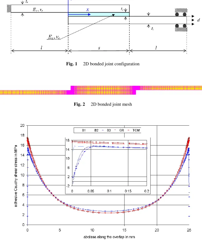
The balanced single-lap bonded joint configuration studied in this paper and its geometrical characteristics are shown in Fig. 1 and Table 1. The adherend material is assumed isotropic linear elastic; the adherends are referred to aluminium [5]. Two different adhesive materials are employed to perform this numerical study: (i) relatively stiff isotropic linear elastic, (ii) hyperelastic. The characteristics of the materials are shown in Table 2.

The FE models used the 2D isoparametric plane strain quadrilateral elements T015 in SAMCEF. A progressive mesh towards the overlap ends was adopted, in order to take into account the stress gradient as well as the singularities

adherends are modelled with five elements in the thickness, while either three or one element is used for the adhesive layer. A plot of the typical mesh is given in Fig. 2. Both degree 1 and 2 of the interpolation functions is under consideration, in order to determine the solution to converge the computation, while satisfying different given criteria. It is remarked that elements of degree 1 in SAMCEF are, by default, internal mode elements, which is an improvement of corresponding traditional elements to better simulate the bending problem. As the rigidity of the adhesive is small compared to the adherends, the selective integration, as proposed in the guideline associated to the SAMCEF FE code

[8], was used in order to overcome the singularities in the stiffness matrix of FE analysis.

The system is clamped at one unbonded adherend end and free to move in the longitudinal direction only at the other end, as shown in Fig. 1. The numerical tests are then controlled in displacement mode, meaning the joint is loaded by imposing a displacement d at the free end. In this study, this imposed displacement is chosen equal to 0.1 mm.

Both geometrical and material nonlinearities are taken into account, in particular for the case of hyperelastic adhesive. The Newton-Raphson resolution algorithm is employed.

2.2 Elastic adhesive

This analysis is conducted using the adhesive 1 (Table 2).

Numerous published works studied the balanced single-lap bonded joint by giving analytical formulation in order to investigate the stress distribution in the adhesive layer. In this study, both the classical approach of Goland and Reissner (GR) [9] and its improved solution by Tsai, Oplinger, Morton (TOM) [10] are employed as indicators of the overall validity of the stress distribution provided by the numerical models. The principle of these previous studies is, at first, to determine the joint edge loads and then to calculate the stress distribution along the overlap considering the edge loads as boundary conditions. Since ta/Ea = 0.1(tr/Er), the structure is considered as a flexible joint according to

GR. In addition to the consistence to the above analytical approaches, in term of stress distribution, the free-stress state at joint ends is considered as an accuracy indicator meaning that the adhesive shear stress decrease to zero towards the end of the overlap. Indeed, even if an adhesive fillet, changing the adhesive stress distribution, is mainly present in bonded joints, the academic adhesive squared end is under consideration, to facilitate the assessment of the simulation accuracy. This latter boundary condition was investigated using minimum strain energy theory by Allman [11] or variational principle of complementary energy by Chen, Cheng [12].

Preliminary numerical tests with different minimum element sizes show that, for our given geometry configuration, minimum size of 0.004 mm for the elements at the overlap end allows for satisfying the free-stress state criterion. Although the aspect ratio reaches the high value of 25:1, the computation provides a convergent solution and coherent results, in terms of the force-displacement behaviour as well as the adhesive stress distribution along the overlap. Moreover, if the aspect ratio increases up to 50:1, the computation remains convergent and the results are still coherent. In this paper, a maximal authorised aspect ratio is then chosen as 25:1.

A significant number of preliminary numerical tests, which are not presented in this paper, were performed by varying the number of elements in the adhesive thickness. These tests show that the stresses are constant across the thickness of the adhesive except at overlap ends due to the free-state boundary condition and the joint singularities, so that the adhesive layer is hereafter modelled with one or three elements in the adhesive thickness. The influence of both the degree of interpolation function and the number of elements employed in the adhesive layer is investigated by the means of three models B1, B2 and B3 (Table 3). In order to perform the comparison both with the analytical approaches and between the three models, which do not take into account to the influence of singularities, the adhesive stresses are measured in the middle of the adhesive layer.

The force-displacement curves are linear until applied displacement of 0.1 mm. The joint stiffness – computed as the slope of the force-displacement curves – given by the model B1, B2, B3 is 1372.6 N.mm-1, 1373.1 N.mm-1 and 1368.4 N.mm-1 respectively. As the maximum relative difference between these values from the one given by B1 is estimated 0.34%, all three models are then considered able to give correct results in terms of joint stiffness.

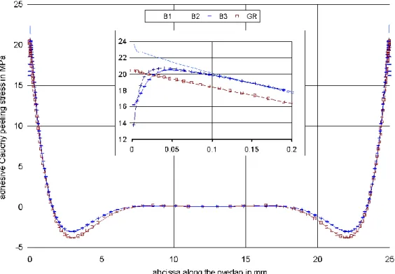
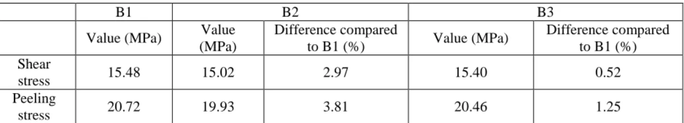
The adhesive stress distributions along the overlap given by the two models B1 and B3 with 3 elements in the adhesive thickness are superimposed, except for very light difference of their peaks close to overlap ends (Fig. 3, 4). As the maximum difference between the peak values (Table 4) is 1.25% for the peeling stress, the degree of interpolation function is considered not to create significant difference of stress distributions, while the adhesive thickness is modelled with three elements. On the contrary, poor results, that are position of maximum shear stress peak (Fig. 3) and in particular value of maximum peeling stress peak (Table 4), are obtained with the model B2 which uses only one element of degree 1 to represent the thickness of the adhesive layer. B1 is therefore considered as the most suitable model because its number of degree of freedom (dof) is approximately 50% of the one of B3. The relative consistence of adhesive stresses distributions given by FE analysis and analytical solutions of GR and TOM are observed (Fig. 3, 4). The comparison of numerical and theoretical results (Table 5) shows that analytical approaches overestimate the value of adhesive stress peaks, in particular shear stress.

2.3 Hyperelastic adhesive

This analysis is conducted using the adhesive 2 (Table 2). A brief review of hyperelastic behaviour is presented in Appendix giving expression of 2- and 3-coefficient Mooney-Rivlin thermodynamic potential. The equivalent Young’s modulus of given material adhesive 2 is equal to 7.2 MPa, or an equivalent shear modulus of 2.6 MPa; the theoretically response of an incompressible hyperelastic behaviour under an uniaxial tensile deformation mode and under a simple shear deformation mode is given in Fig. 5 and Fig. 6 respectively (for C10 = 0.3 and C01 = 0.8). The relative stiffness in

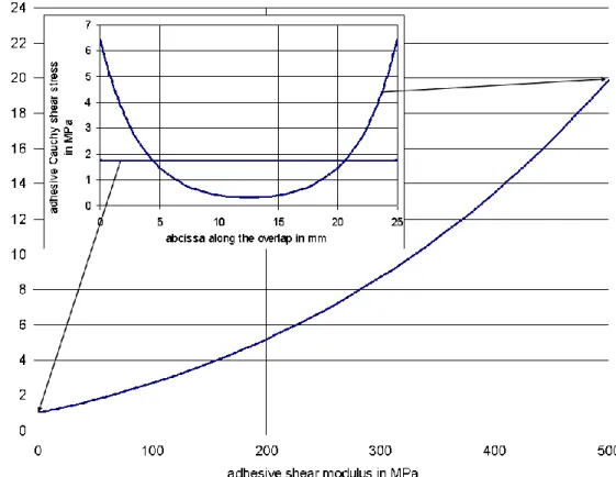
the thickness is then of 45000 MPa.mm-1 for the adherends and of 72 MPa.mm-1 for the adhesive, or 0.16% of the previous value of the adherends. As the prediction of Volkersen [13] (Fig. 7) shows that the difference between the

performed on the joint described in Fig. 1 and Tab. 1 – the simulation using the adhesive 2 is predicted to give a nearly homogeneous adhesive shear stress distribution. Therefore, the minimum size of the element at the overlap ends could be increased, in order to reduce the number of dof, since no significant overstress should be observed at the overlap ends.

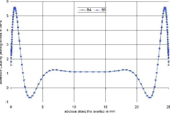
Two new FE models B4 and B5 of degree 1 were created with the minimum element size of 0.004 mm and 0.01 mm respectively. Both models are modelled with three elements in the thickness of the adhesive. The force-displacement curves are linear until an applied force-displacement of 0.1 mm. The joint stiffness given by the model B4, B5 is 434.57 N.mm-1, 434.73 N.mm-1 respectively. The relative difference between these two values from the one given by B4 is estimated 0.04%, which is completely negligible. The two models are considered to give the same global response.

Fig. 7 and 8 present the adhesive shear and peeling stress distributions of the medium element layer along the overlap. The good consistence of the results given by both above models shows that the minimum size of 0.01 mm is enough to obtain a good stress distribution. As predicted, the homogeneous shear stress distribution observed is consistent to the solution given by Volkersen using the equivalent adhesive shear modulus, except for two peaks close to the overlap ends. The value of these maximum peaks is estimated 12% higher than the prediction of Volkersen. The free-stress condition is verified by the decrease to zero of shear stress at the end of the joint. Contrary to the previous case of adhesive 1, both peaks of peeling stress are not located at or almost at the overlap ends but at some distance from them. The distributions of this stress tensor component, as well as of the xx and zz components, are affected by the hydrostatic pressure p, which is directly calculated from the relative variation of volume via the selective integration. This parameter of hydrostatic pressure represents the mechanical response of the nearly incompressible material to volume load and is sensitive to the compressible property characterised by the compressibility modulus Ka.

In order to understand the influence of the adhesive compressibility on the joint behaviour, FE analyses using model B5 with different values of Ka, i.e. 5000 MPa, 1300 MPa, 130 MPa, 52 MPa and 26 MPa, were carried out. Fig. 9 shows a

significant dependence of the peeling stress on Ka. Higher value of Ka, meaning that the material is less compressible,

generates higher values of peeling stress peaks. The shear stress distribution is also modified while varying the value of Ka. The variation of the joint stiffness is small along with the compressibility. Moreover, it is observed that when Ka is

high enough, the response in term of stiffness seems to approach an asymptotic limit. An incompressible material is traditionally approached by nearly incompressible hyperelastic potential using a high value of Ka. A value of 2600 MPa

for Ka corresponds to a value of 0.4995 of a, which could be considered as a good approximation of incompressible

material (a = 0.5). This numerical approach aims at avoiding the singularities in the stiffness matrix during FE analysis.

Therefore, the value of compressibility modulus should be carefully determined by experiments before introducing to FE models in order to analyse joint behaviour. In this paper, the value of 5000 MPa for Ka allows for studying

Hyperelastic material could be modelled with numerous existing thermodynamic potentials. The potentials may give different numerical results of joint stiffness and adhesive stress distribution. In this work, the third parameter C20 is

introduced in order to examine its influence on the joint response. Different values are tested: 0 MPa, 0.005 MPa, 0.01 MPa, 0.05 MPa and 0.1 MPa. The first value of 0 MPa corresponds to the 2-coefficient Mooney-Rivlin potential. In general, as the 3-coefficient potential is a modification of the 2-coefficient one, the value of C20 should be small

compared to the two previous ones C10 and C01. Therefore, the last value tested is fixed at 0.1 MPa. Linear variation of

joint stiffness along with C20 shows that the introduction of this third parameter in the model permits to stiffen the

material and consequently the joint behaviour. Shear stress distribution is almost lightly shifted upwards while the influence of C20 on peeling stress manifests only at its peaks. The increases given by the model with C20 = 0.1 MPa

compared to the 2-coefficient Mooney-Rivlin potential are estimated as 3.10% for joint stiffness, 7.38% for shear stress peaks and 8.42% for peeling stress peaks. The parameter C20 is then considered to lightly stiffen the adhesive material.

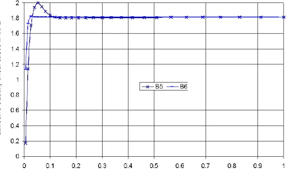
The problem of convergence arises along with the increase of displacement. The negative pivots of the stiffness matrix gradually appear during the numerical resolution and finally make the computation diverge. For our given configuration and materials, the FE analysis using the model B5 diverges at approximately d = 0.5 mm. Two solutions are considered in order to make the FE analyses possible for significant imposed displacement load: (i) modification of computational parameters, (ii) modification of the meshing parameters of the adhesive layer. For the first solution, different allowable time step sizes as well as change in number of iterations for each Newton-Raphson step do not offer any significant improvement in the convergence of the computation. The negative pivots, which appear during the FE analysis, correspond to the nodes lying inside the adhesive layer. A second solution is therefore considered by modelling with only one element in the thickness of the adhesive. As the previous model B2 using 1 element of degree 1 in the adhesive thickness gives very poor results, adhesive elements of degree 2 are employed in order to improve the flexibility of the adhesive layer. The mixed degree model B6, which consists of adherend elements of degree 1 and only one layer of adhesive elements of degree 2, allows the FE computation to converge up to a high value of imposed displacement d. As the difference in term of joint stiffness given by the models B5 and B6 is estimated 0.02%, the mixed degree model is considered to give the correct stiffness value. For adhesive stress results, the difference of peeling stress peaks is estimated 0.02% while it is 8.93% for the shear stress peaks (Fig. 11). Contrary to the model B5, the mixed degree model B6 does not show clear shear stress peaks close to the overlap ends, which explained the significant difference of this stress component given by these two models.

Using SAMCEF to simulate single lap bonded joints with nearly incompressible hyperelastic flexible adhesives in 2D could be carried out with the two above models B5 and B6. For low values of displacement load, the model entirely of degree 1 with 3 elements in the thickness of the adhesive should be used. Once the load is significant, in order to ensure the convergence of the computation, the mixed degree model should be employed.

3. Three-dimensional finite element analysis of single-lap bonded joints with flexible adhesive

3.1 3D FE modelling of single-lap bonded joints

The 3D configuration of single-lap bonded joints results simply from extruding the previous 2D geometry in z or the width direction of joint. In this 3D analysis, the width of joint is chosen as 2w = 25 mm. As the joint configuration is symmetric in relation to the z = 0 plane, only a half of the specimen is modelled. Three boundary conditions are therefore applied: (i) symmetrical condition of the z = 0 plane, (ii) clamping condition at one unbonded adherend end, (ii) free to move in the longitudinal direction only at the other unbonded adherend end. As in 2D analyses, an imposed displacement is chosen as d = 0.1 mm. The flexible adhesive, adhesive 2, is studied in this analysis.

It is demonstrated that negative pivots of the stiffness matrix in the 3D analysis appear earlier than in the 2D case. Therefore, the mixed degree model would be employed. In the previous 2D plane strain analysis, the investigation of stress distribution along the overlap showed that (i) shear stress is almost homogeneous and (ii) peeling stress peaks are located at some distance from overlap ends. Furthermore, the mixed degree model, which would be used in this 3D analysis in order to ensure the computational convergence, does not create any significant overstress close to overlap ends. The minimum element size at overlap ends could then be increased in order to reduce the number of dof, regarding significant increasing size of the 3D model compared to the 2D one. This minimum size is chosen equal to 0.1 mm which is the thickness of the adhesive layer.

The 3D FE analysis aims at studying the variation of adhesive stress in the width, or the influence of the free surface of the specimen. Similarly, in the longitudinal direction, progressive mesh towards the free surface is adopted. As homogeneous shear stress distribution is expected regarding flexible adhesive material system, reasonable minimum size at the free surface, which is not necessarily too small, could be considered. It is then chosen as 0.1 mm, which provides cube elements at the two singular corners of the joints.

The same computational parameters as in the previous analysis in 2D are employed.

3.2 Results and discussion

A linear curve of force-displacement representing global response of the structure is obtained. The joint stiffness given by the 3D model is 421.18 N.mm-1, or 96.88 % of the value given by previous 2D analyses. The decrease in terms of joint stiffness means that the 3D model, which takes into account the influence of the free surface of the specimen, is slightly less stiff than the 2D plane strain model.

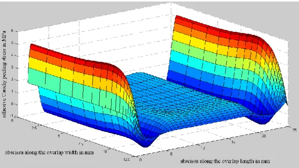
As expected, the shear stress distribution is homogeneous in the overlap (Fig. 12). No significant variation of this stress component due to the free surface of the specimen is observed. The relative difference between maximum and minimum values from the minimum value is estimated as 9.39 %. Contrary to shear stress, the influence of the free stress surface of the specimen is clearly demonstrated by the peeling stress distribution. Fig. 13 shows a sharp decrease of peeling stress at the free surface. In terms of peak values, the difference between 2D (B6 model) and 3D models

relatively to the 3D model is 1.68% for the adhesive Cauchy shear stress and 4.71% for the adhesive Cauchy peeling stress. The above stress analysis affirms that no significant overstress is generated by the consideration of the 3D effects.

4. Three-dimensional finite element analysis of single-lap HBB joints with flexible adhesive

4.1 Three-dimensional modelling of single-lap HBB joints

The previous parts determined some principles in terms of FE simulation techniques of single-lap bonded joints with flexible adhesives which would be applied to single-lap HBB joints. A parametric FE model of single-lap HBB joint is developed by improving the one described in [5] thanks to above principles to better simulate hyperelastic adhesive; in particular, the simulation of bolts is not modified, so that the contact between the adherends and the bolts is then assumed without friction and that no preload is considered.In order to take into account the influence of both free surface and the holes of the adherends, the new HBB model associates two parts: (i) HBB part using transitional mesh around the fastener holes, (ii) bonded part to model the influence of the free surface.

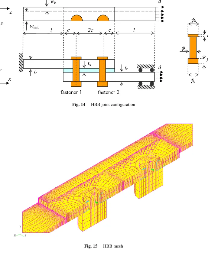
Fig. 14 presents the considered 2-line HBB joint configuration. Its geometrical and meshing characteristics are given in Table 6. Like the bonded part of the model, the HBB part employs the progressive mesh for the overlap in order to refine the model at the overlap ends and the holes as well, without increasing systematically the number of dof. The model is of mixed degree meaning that the adhesive layer is modelled with only one element in the thickness but of degree 2 while the elements of degree 1 are used for adherends. The mechanical interaction between the fasteners and the adherends is modelled by contact elements. As shown in Fig. 15, a good refinement towards the overlap ends and the free surface is adopted for the bonded part while the HBB part is less refined. The minimum element size at the overlap ends as well as at the free surface of the bonded part is chosen equal to 0.1 mm, which is the adhesive layer thickness. The minimum size at the overlap ends and at the fastener holes of the HBB part are chosen equal to 0.2 mm and 0.5 mm respectively.

The screw material is considered isotropic linear elastic of 110 000 MPa for Young’s modulus and 0.33 for Poisson’s ratio, which is referred to a titanium material. The nuts are assumed to be of the same material as the adherends. The flexible adhesive 2 is used in this analysis.

Only a half of the specimen is modelled regarding its symmetry in relation to plane z = 0. Similarly to 3D modelling of single-lap bonded joint, three boundary conditions are then applied to the joints: (i) symmetric condition for plane z = 0, (ii) clamping condition at one unbonded adherend end, (ii) free to move in the longitudinal direction only at the other unbonded adherend end. The imposed displacement is chosen as 0.3 mm corresponding to a value of nearly 50 MPa for the applied stress, which is expected not to create any plastic deformation in the adherends.

4.2 Results and discussion

4.2.1 Adhesive stresses

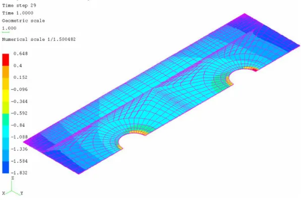
An almost good continuity at the connection of the two parts of the model in term of adhesive stress distribution is obtained. Adhesive shear stress is, as predicted, homogeneous in the overlap except at the fastener holes due to the stress concentration (Fig. 16). On the contrary for peeling stress distribution (Fig. 17), another overstress is observed at the overlap ends on the connection line of the two parts of the model, which could be explained by the mesh quality. Indeed, the transition ratio, which is representative of the ratio between the sizes of two consecutive elements, is maximum on the connection line and at the overlap ends and is equal to 20. Nevertheless, high transition ratios are obtained in a very restricted zone (Fig. 15).

4.2.2 Bolt load transfer rate

In HBB joints, the load is transferred from one adherend to the other via the adhesive layer and the fasteners. As a discrete mode, the transfer by fasteners is characterised by its load transfer rate, which is defined as the ratio between the load transferred by the fastener and the applied load. In order to calculate these transfer rates of the fasteners, the special method presented in [4] is employed, which consists in summing the nodal forces on the mid-surface of the bolt.

The transfer rates are of 0.337 for fastener 1 and 0.339 for fastener 2, meaning that the adhesive layer transfers almost one third of the applied load. As the joint configuration is not completely anti-symmetric, a small relative difference from the result given by fastener 1 of 0.6 % in term of transfer rate is observed between the two fasteners.

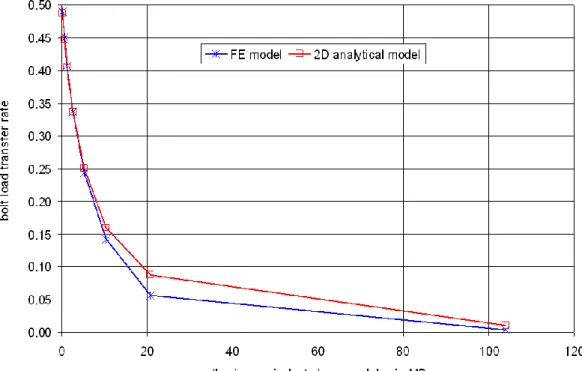
The 2D analytical model developed in [5] is able to predict the bolt load transfer rate in HBB joint with isotropic linear elastic adhesive. In this model, the fasteners are characterised by their shear and bending stiffness which could be calculated one from another thanks to the method given in [5]. Thanks to the 3D numerical simulation, the shear stiffness is determined by correlating the numerical and the analytical results at a specific value of bolt load transfer rate which is chosen, in this study, as the result given by the FE analysis using the adhesive 2. Fig. 18 shows the evolution of bolt load transfer rate with the adhesive equivalent shear modulus given by (i) FE analysis and (ii) 2D analytical model of [5] by varying the adhesive material. A very good correlation between both approaches is obtained for high values of bolt load transfer rate. As the adhesive is stiff enough, meaning the role of the fasteners is no longer significant in terms of load transfer, the results given by both approaches are slightly different.

4.2.3 Coefficient of stress concentration for bolted lap joints

It is supposed that bolted joints, of which a sealant layer is employed for sealing, could be simulated by a HBB joint, for which the adhesive stiffness is low enough, so that the applied load is almost transferred by the bolts. For bolted lap joints, stress concentration obviously appears due to the presence of the holes in the adherends. Since lateral pressure or preload is not considered in the presented FE analysis, the critical stress concentration is located at the root

of the fastener holes nearest to the applied load ends. The coefficient of stress concentration is computed as the ratio between the first principal stress, which is considered as the responsible component to open the initial crack, at the considering point and the applied stress. This coefficient of stress concentration serves fatigue analysis of the structure.

It was showed by Homan and Jongebreur [14] that, for bolted lap joints, the stress concentration results from three contributions: (i) load transmission by the fastener, (ii) bypass load and (iii) secondary bending, as shown in the following equation:

Kt =  Kt, pin + (1-)Kt, hole, tension + kKt, hole, bending (1)

where Kt is the stress concentration to be calculated, k is the secondary bending factor,  is the bolt load transfer rate

and Kt, pin, Kt, hole, tension, Kt, hole, bending are the stress concentration factors of the three above contributions respectively. In

order to simplify the analysis, the stress contribution of bending is neglected, so that the coefficient of stress concentration results from the contribution of both load transmission and bypass load only, in a same way as described by Niu in [15]. Kt, pin and Kt, hole, tension depend on the joint geometry only and could be deduced from the dedicated tables

provided in [15]. Experimental curves in [15] show that the higher stress concentration generated at the fastener holes, the shorter fatigue life could be sustained by bolted joints.

4.2.4 Fatigue life of HBB joints – Comparison with corresponding bolted joints

In the frame of this paper, the fatigue life of HBB joints is simply compared to bolted joints in order to prove, in a numerical approach, that the mechanical performance of the HBB joining technology is better than classical bolted joints.

The fatigue strength of the adhesive layer is not addressed in this paper. The fatigue performance analysis is then restricted to HBB joints, for which the critical zones are located at bolt holes rather than at the overlap ends. The adhesive is supposed flexible, meaning that it is able both to sustain large deformation and to be characterized by low stifnness, so that HBB joints are assumed not to create both failure in the adhesive layer and sufficiently high overstress in the adherends. Consequently, the variation of Kt as a function of  is investigated for the HBB configuration.

In order to obtain different values of , the adhesive material is varied by considering C01 = 1.6 C10 with C10 =

0.0289, 0.125, 0.25, 0.5, 1, 2, 4 and 20 MPa. . It is observed that the stress concentration factor increases linearly with the bolt load transfer rate for approximately from 0.05 to 0.45. The slight difference between the two curves, corresponding to fastener 1 and fastener 2 (Fig. 19), should be explained by the imperfectly anti-symmetrical configuration of the joint. Since stress concentration at the hole of fastener 1 is more critical than fastener 2 (Fig. 19), the failure of our HBB joint should occur in the adherends at the fastener 1 head side. According to the evolution of stress concentration coefficient with bolt load transfer rate (Fig. 19), HBB joints generate lower value of Kt than

corresponding bolted joints. Fatigue life of HBB joints is therefore longer than bolted joints, while the critical sites are located at fastener holes.

5. Conclusions

Single-lap bonded and HBB joints with flexible adhesives are simulated in 2D plane strain and in 3D using SAMCEF FE code. Hyperelastic 2- and 3-coefficient Mooney-Rivlin potentials are used to model the behaviour of the adhesive. The influence of different parameters on the behaviour of joints is carried out. The viscoelasticity of the adhesive material is studied as well. The principal conclusions of the present study are:

1. Mixed degree FE models, which combine one element of degree 2 in the adhesive thickness with the elements of degree 1 for the adherends, are able to ensure the convergence of the analyses until significant value of displacement load while giving good results in terms of both global and local responses.

2. Since the adhesive is flexible, the adhesive shear stress is homogeneous in the overlap. On the contrary, the distribution of peeling stress, with two clear peaks locating at some distance from the overlap ends, is dominated by the compressibility of the adhesive material. The peeling stress decreases significantly as the free surface of the specimen is approached.

3. Significant influence of the adhesive compressibility on the joint stiffness as well as adhesive stress distribution, in particular on peeling stress, is demonstrated. The introduction of C20 parameter lightly affects the mechanical responses

of the bonded joints.

4. The evolution of stress concentration coefficient with bolt load transfer rate is almost linear for a wide range of . This allows us to conclude that the fatigue life of HBB joints is longer than for corresponding bolted joints.

Nomenclature

Cij : coefficient ij of the Mooney-Rivlin’s potential model in MPa

d : applied displacement in mm

Ea : Young’s modulus of the adhesive in MPa

Er : Young’s modulus of adherends in MPa

k

I : kth reduced invariant of Green-Lagrange strain tensor k : secondary bending factor

Ka : compressibility modulus of the adhesive in MPa

Kt : coefficient of stress concentration

p : hydrostatic pressure in MPa

tr : thickness of adherends in mm

w : half width of the overlap in mm

W : hyperelastic potential

x, y, z : direct orthonormal base

  bolt load transfer rate

a : Poisson’s ratio of the adhesive

Acknowledgements

The authors gratefully acknowledge the engineers of the Methods and Research team of SOGETI High Tech Fatigue & Damage Tolerance Department in Toulouse for their support and advice, in the frame of the development of JoSAT (Joint Stress Analysis Tool) internal research programme.

Appendix: Mooney-Rivlin potential model for hyperelasticity

Nearly incompressible hyperelastic behaviour is characterised by a thermodynamic potential:

)

,

,

(

I

I

I

W

W



I

,

I

,

I

2- and 3-coefficient Mooney-Rivlin potential are given by the following formulae:

 

 

where Ka is the compressibility modulus.

References

[1] Hart-Smith LJ. Design methodology for bonded-bolted composite joints. Technical Report AFWAL-TR-81-3154. Douglas Aircraft Company. 1982

[2] Imanaka M, Haraga K, Nishikawa T. Fatigue Strength of Adhesive/Rivet Combined Lap Joints. Journal of Adhesion 1995; 49:197-209

[3] Fu M, Mallick PK. Fatigue of hybrid (adhesive/bolted) joints in SRIM composites. International Journal of Adhesive & Adhesion 2001; 21:145-159

[5] Paroissien E, Sartor M, Huet J. Hybrid (Bolted/Bonded) Joints Applied to Aeronautic Parts: Analytical One-Dimensional Models of a Single-Lap Joint. Trends and Recent Advances in Integrated Design and Manufacturing in Mechanical Engineering II, Springer Eds., ISBN978-1-4020-6760-0 October 2007, pp.95-110

[6] Paroissien E, Sartor M, Huet J, Lachaud F. Analytical Two-Dimensional Model of a Hybrid (Bolted/Bonded) Single-lap Joint. Journal of Aircraft 2007; 44:573-582

[7] Crocker LE, Duncan BC, Hughes RG, Urquhart JM. Hyperelastic Modelling of flexible adhesives. NPL Report CMMT(A)183. ISSN 1361-4061, May 1999

[8] SAMCEF. Version 11.1-04. Samtech Group, Liège, Belgium, 31st August 2006

[9] Goland M, Reissner E. The stresses in cemented joints. Journal of Applied Mechanics 1944; 11:A17-27

[10] Tsai MY, Oplinger DW, Morton J. Improved theoretical solutions for adhesive lap joints. International Journal Solids Structures 1998; 35:1163-1185

[11] Allman DJ. A theory for elastic stresses in adhesive bonded lap joints. Quarterly Journal of Mechanics and Applied Mathematics 1977; 30:415-436

[12] Chen D, Cheng S. An analysis of adhesive-bonded single-lap joints. Journal of Applied Mechanics 1983; 50:109-115

[13] Volkersen O. Die Niektraftverteiling in Zugbeanspruchten mit Konstanten Laschenquerchritten. Luftfahrtforschung 1938; 15:41

[14] Homan J, Jongebreur AA. Calculation method for predicting the fatigue life of riveted joints. Durability and Structural Integrity of Airframes. Proc. 17th ICAF Symposium, Ed. A.F. Blom. EMAS (1993) pp.175-190

Fig. 1 2D bonded joint configuration

Fig. 2 2D bonded joint mesh

Fig. 4 Adhesive peeling stress distribution along the overlap of models B1, B2, B3, GR

Fig. 5 Response of an incompressible hyperelastic material subjected to uniaxial tensile deformation

Fig. 6 Response of an incompressible hyperelastic material subjected to simple shear deformation

(obtained with C10 = 0.5 and C01 = 0.8 and varying values of C20)

Fig. 8 Adhesive shear stress distribution along the overlap of models B4, B5, Volkersen

Fig. 10 Adhesive peeling stress distribution for different values of compressibility modulus

Fig. 12 Adhesive shear stress distribution in the overlap

Fig. 14 HBB joint configuration

Fig. 16 Adhesive shear stress distribution according to the HBB model

Fig. 18 Evolution of bolt load transfer with adhesive equivalent shear modulus

Table 1 2D bonded geometrical parameters

l (mm) s (mm) tr (mm) ta (mm)

30 25 1.6 0.1

Table 2 Material parameters

Material Isotropic linear elastic Hyperelastic (Mooney-Rivlin potential) Young’s Modulus (MPa) Poisson’s ratio  First parameter C10 (MPa) Second parameter C01 (MPa) Compressibility modulus K (MPa) Adherend 72000 0.33 Adhesive 1 450 0.33 Adhesive 2 0.5 0.8 5000

Table 3 Description of models B1, B2, B3

Model Number of elements in the adhesive thickness Degree of interpolation functions of adhesive elements Degree of interpolation functions of adherend elements B1 3 1 1 B2 1 1 1 B3 3 2 2

Table 4 Stress results of models B1, B2, B3

B1 B2 B3

Value (MPa) Value (MPa) Difference compared to B1 (%) Value (MPa) Difference compared to B1 (%) Shear stress 15.48 15.02 2.97 15.40 0.52 Peeling stress 20.72 19.93 3.81 20.46 1.25

Table 5 Stress results of B1, GR, TOM

B1 GR TOM

Value (MPa) Value (MPa) Difference compared to B1 (%) Value (MPa) Difference compared to B1 (%) Shear stress 15.48 17.51 13.11 17.01 9.88 Peeling stress 20.72 20.44 1.35

Table 6 HBB joint geometrical parameters

l (mm) c (mm) tr (mm) ta (mm) whbb (mm) wb (mm) h (mm) b (mm) n (mm) hh (mm) hn (mm) 178 12 1.6 0.1 8 4 7.2 4.8 10.08 1.155 6.6