HAL Id: hal-00855409
https://hal.archives-ouvertes.fr/hal-00855409
Preprint submitted on 29 Aug 2013
HAL is a multi-disciplinary open access
archive for the deposit and dissemination of
sci-entific research documents, whether they are
pub-lished or not. The documents may come from
teaching and research institutions in France or
abroad, or from public or private research centers.
L’archive ouverte pluridisciplinaire HAL, est
destinée au dépôt et à la diffusion de documents
scientifiques de niveau recherche, publiés ou non,
émanant des établissements d’enseignement et de
recherche français ou étrangers, des laboratoires
publics ou privés.
Ground Moving Target Trajectory Reconstruction in
Single-Channel Circular SAR
Jean-Baptiste Poisson, Hélène Oriot, Florence Tupin
To cite this version:
Jean-Baptiste Poisson, Hélène Oriot, Florence Tupin. Ground Moving Target Trajectory
Reconstruc-tion in Single-Channel Circular SAR. 2013. �hal-00855409�
Abstract—Synthetic aperture radar has become an important
technique for generating high-resolution images of the ground, because of its all-weather capabilities. SAR imaging of stationary scenes is nowadays well mastered. If targets are moving, it induces a delocalization and a defocusing effect in the azimuth direction in a SAR image. This last effect can be used to detect moving targets, to image them and to estimate their azimuthal velocity, but the main limitation is the impossibility to estimate the full target velocity vector, because of the Doppler shift dependency on azimuthal position and radial velocity.
The purpose of this paper is to use several aspect angles thanks to a circular trajectory acquisition to retrieve the entire velocity and position vector. We first outline the steps of this trajectory reconstruction methodology, then we perform a mathematical analysis of this methodology and finally we present some tracking results on real data, around two French cities.
I. INTRODUCTION
ynthetic aperture radar has become an important technique for generating high-resolution images of the ground, because of its all-weather capabilities. SAR imaging of stationary scenes is nowadays well mastered [1] but if a moving target is present in the illuminated scene, it appears delocalized in the azimuth direction and defocused in the SAR image [2].
Two main SAR processing categories have been considered in the recent literature. The first category concerns moving target detection and tracking with multiple aperture antennas SAR. This category relies on Displaced Phase Center Array (DPCA) [3], Space-Time adaptive processing (STAP) [4], along-track interferometry (ATI) [5] and detection by focusing using different full velocity vector hypothesis [6]. One advantage of these techniques is the ability to suppress clutter. The detection of moving targets is therefore made easier, especially in severe background environment [7, 8].
This paragraph of the first footnote will contain the date on which you submitted your paper for review. It will also contain support information, including sponsor and financial support acknowledgment. For example, “This work was supported in part by the U.S. Department of Commerce under Grant BS123456”.
The next few paragraphs should contain the authors’ current affiliations, including current address and e-mail. For example, F. A. Author is with the National Institute of Standards and Technology, Boulder, CO 80305 USA (e-mail: author@ boulder.nist.gov).
S. B. Author, Jr., was with Rice University, Houston, TX 77005 USA. He is now with the Department of Physics, Colorado State University, Fort Collins, CO 80523 USA (e-mail: [email protected]).
T. C. Author is with the Electrical Engineering Department, University of Colorado, Boulder, CO 80309 USA, on leave from the National Research Institute for Metals, Tsukuba, Japan (e-mail: [email protected]).
Moreover, these techniques estimate the slant-range velocity of the moving target. Therefore, a combination of the above methods is efficient to retrieve the full velocity vector of the moving targets [8].
For practical reasons, a significant part of airborne SAR systems is limited to one single channel. The SAR systems developed by the French Aerospace Lab ONERA (SETHI [9], and more recently RAMSES NG [10]) fit into this category. Standard single antenna processing exploits the moving target apparent characteristics to focus them [11, 12] and estimate their azimuth velocity [13] under the assumption of a high PRF, in order to avoid the Doppler ambiguity problem [14]. The main limitations of these methods are:
1) The impossibility to estimate the full target velocity vector, because of the Doppler shift dependence on both azimuthal position and radial velocity of the moving target [15].
2) The errors in the azimuthal velocity estimate due to the background image [11].
Some interesting studies have been done on ground moving target tracking in single channel SAR to solve this problem. Kirscht [16] uses the information content of multilook processing [17] to detect potential moving targets. The full target velocity vector is then estimated from target displacement between successive images with a normalized cross correlation function as matching criterion [18]. Dias and Marques [19] propose to use the amplitude modulation term of the returned echo from a moving target to estimate its radial velocity, and then avoid the azimuth ambiguity. The radial velocity estimator used in [19] yields effective results for a high signal-to-clutter (SCR) ratio (14 dB), but in most cases in urban context, the SCR is lower than 14dB. The velocity estimation with a cross correlation function [16, 18] could be imprecise in the case of defocused targets and the moving target trajectory estimation can thus be flawed. Furthermore, the radial velocity estimation given the antenna radiation pattern [14] is affected by the clutter, the anisotropic behaviour of the moving targets and the weak directivity of the beam.
Acquisitions of SAR data over a circular trajectory [20] bring new information, because objects may be seen from any aspect angle. The continuity of the SAR-plateform movement may thus enhance moving targets trajectory reconstruction, because objects of interest may be seen during a longer time than in the linear stripmap SAR case. Thanks to the multiple azimuth direction, the azimuth ambiguity may be solved. A
Ground Moving Target Trajectory
Reconstruction in Single-Channel Circular SAR
J.B. Poisson, Student Member, IEEE, H. Oriot, and F. Tupin, Senior Member, IEEE
method proposed in [21] uses multiple backprojection images as input of a framework called Dynamic Logic. This framework computes the maximum likelihood ratio between moving target Gaussian models and data, providing moving target detection and characterization. In this paper, we suppose that targets have already been detected which means that their backscattering level is high enough to encompass any defocusing effect. Having SAR images acquired along a circular trajectory in spotlight mode, we present an inversion method to retrieve the target ground position and velocity from the apparent coordinates of the moving targets in these SAR images and the estimated azimuthal velocity.
This paper is organized as follows. In section II we outline the steps of our trajectory reconstruction methodology. In section III we perform a mathematical analysis given synthetic data and finally we present in section IV some trajectory reconstruction results on real data, around the city of Nîmes (acquired by the SAR system SETHI) and around the Istres Airport (acquired with RAMSES NG) in France.
II. MOVING TARGET TRACKING METHODOLOGY
In this section, we describe the image geometry, then we present the moving target model, we describe the measurement method, we explain how the whole trajectory of the moving target is reconstructed given its apparent coordinates in the SAR images and under several moving target hypotheses, and then we present the system inversion calculation using the Least Mean Squares (LMS) method. A. SAR acquisition geometry
Let us consider the SAR scenario illustrated in Fig. 1 where the SAR plateform moves along a circular trajectory, so that SAR images can be computed for all possible azimuth angles. Images are processed in a spotlight mode, so each azimuth direction corresponds to a squint angle.
B. Moving target 2nd order model
We consider a moving target with velocity ⃗ and acceleration , which is considered to be constant during the sensor displacement between and . The SAR-plateform velocity is noted ⃗⃗⃗ and its acceleration is noted ⃗⃗⃗⃗ . In this section, we consider that the moving target is a point-like isotropic scatterer for the calculation of the target phase history. Real moving targets are actually made up of finite number of bright spots, whose spatial distributions are unpredictable, and depend on the target nature and on the aspect angle. However, for small integration angles, the point-like isotropic scatterer is a good approximation for the moving targets. The method used to calculate the moving target phase history is given by [2] and explained here to present our notations.
At time (resp. ), the target is at position (resp. , see Fig. 1). The phase of the returned echo during the time period is given by:
(‖ ⃗⃗⃗⃗⃗⃗⃗⃗⃗ ‖ ‖ ⃗⃗⃗⃗⃗⃗⃗⃗⃗⃗ ‖) (1)
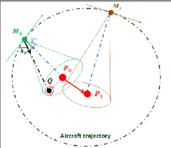
Fig. 1: principle of calculation of two different images. For the first image (resp. the second), the SAR-plateform is in (resp. in ) and the moving target is in (resp. in ). is a still target which appears at the same position as (due to effects of target motion) on the SAR image.
Let
⃗⃗⃗⃗ ⃗⃗⃗⃗⃗⃗⃗⃗⃗⃗
‖ ⃗⃗⃗⃗⃗⃗⃗⃗⃗⃗ ‖ (2)
be the normalized line of sight (LOS) vector for moving target at time . We also define ‖ ⃗⃗⃗⃗⃗⃗⃗⃗⃗⃗ ‖ the distance between the SAR sensor and the moving target at time . A development to the second order in is done, because most of the phase error due to target motion is given by second order terms [11]. For high order studies, see [8]. Adapting the range variation expression with time given by [2] to the case of a circular flight path, we then have:
( ) (3) With: ( ) ⃗⃗⃗ ⃗ ⃗⃗⃗⃗ ( ⃗⃗⃗⃗ ) ( ⃗⃗⃗ ⃗⃗⃗⃗ ) ( ⃗⃗⃗⃗ ⃗ ) ( ⃗⃗⃗ ⃗⃗⃗⃗ ⃗⃗⃗⃗ ⃗ ) (4) ( ) ⃗⃗⃗⃗ ⃗ ⃗⃗⃗ ⃗⃗⃗⃗ (5) Where is the magnitude of ⃗ and is the magnitude of . ( ) is a phase slope in the azimuth frequency domain that induces the azimuth shift of the target. The moving target appears at the same position as a still target on the SAR image. So when we compute the azimuthal spectrum of the moving target , the residual phase is the difference between the phase history of the moving target and the phase history of the still target . Given ⃗⃗⃗⃗ ⃗⃗⃗⃗⃗⃗⃗⃗ ‖ ⁄ ⃗⃗⃗⃗⃗⃗⃗⃗⃗⃗ ‖, we thus have: ( ) (6) With: ( ) ⃗⃗⃗ ⃗ ⃗⃗⃗⃗ ( ⃗⃗⃗⃗ ) (7)
( ) ( ( ) ⃗⃗⃗ ⃗⃗⃗⃗ ) (8) The difference of squint angles between and is zero, so the difference of slope of the phase history is zero ( ), which leads to the relationship:
( ) ( ) (9)
Where and are the projections of moving target velocity in the range and azimuth direction and (resp. ) is the squint angle for the moving target (resp. for the still target ). is the magnitude of the SAR-plateform velocity ⃗⃗⃗ . It should be noted that is linked to the azimuth pixel line corresponding to the centre of the target on the image.
Besides, is an expression which is function of both the velocity component of the moving target in azimuth direction and its radial acceleration. In order to measure , we use the method described in [22]: we first compute the azimuthal spectrum of the moving target. As the phase history of the moving target is developed to the second order in (see equation (6)), we fit a parabola to its phase behavior. We then use an autofocus algorithm which selects the best phase correction, i. e. which selects (see (7)) to be the parameter that best refocuses the moving target in the SAR image.
Finally the ground moving target P appears on a SAR image at the apparent coordinates ( ) with the defocusing parameter . These three measurements lead to the following system: { ‖ ⃗⃗⃗⃗⃗⃗⃗⃗⃗⃗ ‖ ⃗⃗⃗⃗⃗⃗⃗⃗⃗⃗ ⃗ ( ( ) ) (10)
With ⃗⃗⃗ (⃗⃗⃗⃗ ⃗⃗⃗ ). Due to the number of unknowns
( ), we need at least two sets of equations to
solve the problem. A general overview of the model implementation is given in [23]. From now on the system unknowns will be expressed in the Cartesian system ( ), the axis representing the East direction and the axis representing the North direction.
C. Moving target trajectory reconstruction methodology Suppose that SAR images are computed with an angular span corresponding to a time interval . We propose to define a moving target model with constant acceleration during the time , being the number of images used. Moreover, we consider that the target velocity and acceleration are collinear, so we look for targets moving along a straight line during calculation time. The moving target orientation is noted .
Using this hypothesis, we obtain a relationship between the ground coordinates of the moving target in the first image ( ) and those in the following image ( ) and we can use the system (10) for all the images between and to obtain
the full coordinates ( ) of the moving target on the first image.
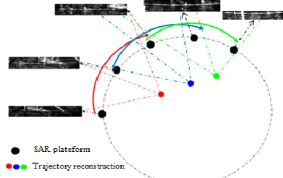
By propagating this principle along the entire circular trajectory (see Fig. 2) of the SAR plateform, we can reconstruct the whole trajectory of the moving target.
Fig. 2: Principle of reconstruction of the moving target whole trajectory. In this example, calculations of the moving target positions are made up of three apparent positions on SAR images.
D. Inversion of the system
Let be the vector containing the output parameters and the measurement vector. corresponds to the moving target ground coordinates and is defined in the general case by:
( ) [ ] ( ) (11) Where denotes vector or matrix transpose and the orientation of the moving target. is given by:
( ) [ ] ( ) (12) The moving target trajectory is obtained by minimising the following function:
( ) ∑ ( )
(13) Where are the equations used for system solving (10), and the number of used images. The minimization of (13) is computed by the Least Mean Squares (LMS) method.
III. VALIDATION ON SYNTHETIC DATA
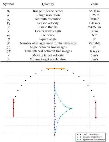
A. Generation of a perfect synthetic aircraft trajectory In order not to take into account the aircraft turbulences, we generate a perfect synthetic aircraft with characteristics close to the reality for the system validation. So we consider that the altitude of the plane is constant during the whole flight, and we consider that the ground altitude is also constant and equal to zero. We consider a moving target with constant velocity towards North. The main characteristics of the aircraft trajectory and of the moving target are summarized in the Table I.
B. Inversion with synthetic moving targets
In this section, we validate the inversion system and we test its robustness. We present the result obtained with the moving target described in the Table I, knowing that other synthetic trajectories were considered. We first compute the apparent trajectory of the synthetic moving target, and then we
test two different types of measurement perturbations. In the first case, we add Gaussian noise to the apparent coordinates ( ), and in the second case we add a sinusoidal perturbation to the target trajectory. For the second case, the aim is to test the inversion robustness if the target behaviour does not perfectly match with the moving target model (the amplitude of the perturbation is equal to and the time period is , with the time interval between two images). This second perturbation and the corresponding apparent trajectory is represented Fig. 3. The moving target trajectory is then estimated with the above-described methodology, given different angular spans. Two different moving target models are used: the first one is a model of a moving target with constant velocity during the computation time interval, and the second is a model with constant acceleration and colinearity constraint.
TABLEI
SYNTHETIC AIRCRAFT TRAJECTORY AND TARGET PARAMETERS
Symbol Quantity Value Range to scene center 5500 m
Range resolution Azimuth resolution 0.25 m 0.002° Sensor velocity Circle Radius 120 m/s 4763 m Center wavelength 3 cm Incidence 60° Squint angle 0°
Number of images used for the inversion Angle between two images Time interval between two images
Variable Moving target velocity 5 m/s Moving target acceleration 0 m/s
Fig. 3 : Representation of a synthetic target trajectory (blue) with a sinusoidal perturbation, and its corresponding apparent trajectory (cyan). The positions of the sensor are represented in black. The points of the real and apparent trajectories highlighted in red, orange and brown exhibit particular behaviors corresponding to the sensor positions marked with red (azimuth configuration), orange (radial configuration) and brown (azimuth configuration) arrows.
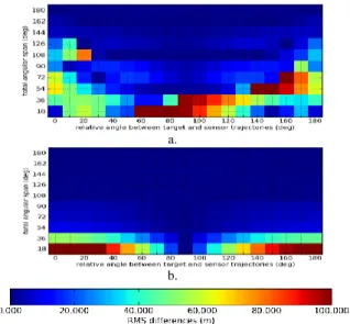
We show the RMS differences between the estimated trajectory and the synthetic ground truth, given the apparent coordinates with the Gaussian noise (see Fig. 4) and with the sinusoidal perturbation (see Fig. 5). The two different moving target models (constant velocity and constant acceleration) are
used. We tested different angular span to invert the system, the maximum angular span is 180°. The axis represents the relative angle between sensor velocity and target velocity, and the axis represents the total angular span used for inversion, given by
. We generate independent data in order to make the mathematical analysis of the system easier (the measurement covariance matrix is diagonal in this case). As we want an azimuth resolution corresponding to the resolution of our real data (which is equal to 0.002°, approximately), the corresponding interval angle between two images is given by:
(14)
In this case, is approximately equal to , so we choose an interval angle equal to .
We see clearly that when we use the moving target model with constant acceleration, the trajectory estimation is more disturbed (position RMS errors mean about ) than with the moving target model with constant velocity (position RMS error about ) for the two perturbations. So the moving target model with constant acceleration is highly sensitive to noisy measurements and to deviations from the moving target model. The results with the sinusoidal perturbation also show that with the target model with constant velocity, from a certain angular span ( in this case), the estimated trajectory is close to the ground truth (position RMS errors ).
We can also notice that the difference of orientation between sensor velocity and target velocity has an influence over the trajectory reconstruction. Indeed, an accurate trajectory reconstruction requires a larger angular span when the moving target is in an azimuth configuration (the difference of orientation is equal to or close to ) than when it is in a radial configuration (the difference of orientation is equal to or close to ). Indeed, when the moving target is in a radial configuration (orange point on the Fig. 3), the moving target is not defocused ( ), so it brings an information of direction of the moving target to the inversion system. Therefore, in radial configuration, we need less measurements to identify the real trajectory of the target from all other possible scenarios.
a.
b.
Fig. 4: RMS differences between the estimated trajectory and the synthetic ground truth, which is a moving target with constant velocity (
of a target with constant velocity. The apparent coordinates of the moving target are disturbed by an additional Gaussian noise ( ).
a.
b.
Fig. 5: RMS differences between the estimated trajectory and the synthetic ground truth. a.: case of a moving target with constant acceleration. b.: case of a target with constant velocity. A sinusoidal perturbation is added to the ground trajectory.
C. Study of the robustness
In order to demonstrate the limitations of the constant acceleration model, we perform a Principal Component Analysis (PCA) of the system (10). Let us consider a matrix expression of this system:
(15)
Because of the non-linearity of the system, the estimate of the output parameters ̂ cannot be analytically given with respect to . By the implicit function theorem, there is a function which satisfies ̂ ( ) and maps the measurements into an estimate of ̂. By non-linear least squares minimization of (15), we obtain an expression of the covariance matrix of the output parameters:
( ̂) ( ) ( ) (16)
Where denotes the measurements covariance matrix. The calculation in [24] gives:
( ) ( ( )) ( ( )) (17) Where ( ) and ( ) . represents the matrix of first partial derivatives of the inversion system (10) with respect to :
(
( )) [ ] [ ] (18) represents the matrix of first partial derivatives of the inversion system (10) with respect to measurements :
(
( ))
[ ] [ ]
(19) And is the exact solution of the system (10). These expressions give an estimation of ( ̂) with only first partials of the system (10), separating those with respect to measurements and those with respect to output parameters. The analytical expressions of and are very complex.
Therefore, we perform a numerical analysis of these matrices. can be factorized as follows, using a Singular Value Decomposition (SVD):
(20)
With a unitary matrix whose columns correspond to the output space. is a diagonal matrix of the non-zero singular values of :
{ (21) With the singular values of . These singular values verify:
⃗⃗⃗ ⃗⃗⃗ (22) The system kernel is thus given by the vectors ⃗⃗⃗ verifying:
⃗⃗⃗ (23)
In order to determine the system kernel, we compute the partial inertia of each vector . This partial inertia is defined
as follows:
∑ (24)
Fig. 6 shows an example of the PCA of the inversion system with a moving target model with constant acceleration and colinearity. The results are represented on a logarithmic scale. The synthetic moving target is the same as the one described in Table I. The partial inertia of each singular value is represented with respect to the angular span (from 0 to 180°). These results (and simulations with other synthetic trajectories) show that even with a large angular span, the partial inertia of the singular value (black curve) is very low ( ) even with a large angular span. So the system kernel is the vector ⃗⃗⃗⃗ , which corresponds to the moving target orientation ( ⃗⃗⃗⃗ ⃗⃗⃗⃗⃗⃗⃗⃗⃗⃗⃗⃗⃗⃗ , with ⃗⃗⃗⃗⃗⃗⃗⃗⃗⃗⃗⃗⃗⃗ the unit vector corresponding to in the observation basis ( ). These curves show the difficulties to reconstruct the target trajectory if the acceleration is a degree of freedom.
Fig. 6: PCA of the inversion system (model with constant acceleration hypothesis and colinearity) given a moving target with constant velocity (5 m/s towards West). The partial inertia of the singular value (red ellipse) is very weak, even with a large angular span.
A PCA is computed again on the system with the same moving target, but with a constant velocity model. The results
0.00001 0.001 0.1 10 0 50 100 150 200
Par
tial in
er
tia
(%
)
Angular span (°)
s1 s2 s3 s4 s5of the PCA with the partial inertia of the 4 new singular values are presented Fig. 7. All the singular values bring significant information from a certain angle (the lowest singular value , which corresponds to the moving target velocity is greater than if the angular span is greater than ). All the results about PCA confirm the results observed on the Fig. 4 and Fig. 5.
Fig. 7: PCA of the inversion system (model with constant velocity). All singular values bring significant information (from a certain angle, the lowest is higher than 1%).
D. Conclusion on synthetic data
In this part, we proposed to validate the moving target trajectory reconstruction methodology, testing two different moving target models: one with constant acceleration and one with constant velocity, both of them considering targets moving along a straight line during calculation time. We performed inversion with synthetic trajectories, testing different measurement noises. The results show a high sensitivity of the constant acceleration model to measurement errors, and these observations are confirmed by a mathematical analysis of the system. We can suppose that the results on real data will confirm these observations.
IV. EXPERIMENTAL RESULTS ANALYSIS
In this section, we present some results concerning real moving target tracking around the city of Nîmes and Istres (two cities in the South of France). We first present the opportunity data sets and then we show the results about target trajectory reconstruction.
A. Presentation of the data sets
We now test the moving target tracking methodology on real SAR data, acquired along circular trajectories. The data were acquired with two different sensors from ONERA,
t
he SETHI sensor and the new sensor RAMSES NG.The new RAMSES NG sensor [10] is dedicated to defense and security applications. The main improvement is the ability to operate as long range and ultra-high resolution in X band. One opportunity data was acquired in Istres area in 2012, and we focus on X band data which have a 50 cm slant range resolution. We examine a moving target (Fig. 8) with ground truth (GPS data). The vehicle is a Renault Master with an average speed of .
The SETHI sensor [9] is an airborne radar more dedicated to civilian applications, equipped with different bands (P, L, X) on a Falcon 20. In this paper, we focus on the X data acquired around the city of Nîmes in 2009, which have a 12 cm slant range resolution. We particularly examine a moving target with unknown trajectory which is supposed to be a train: we see several horizontal lines probably due to train cars. The residual curvature of the horizontal lines is due to
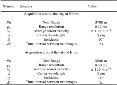
range migration, which appears on images with high azimuth resolution (see Fig. 8). The main characteristics of the two acquisitions are summarized by the Table III.
a. b.
Fig. 8: examples of signatures of moving targets on SAR images at the city of Nîmes (a.) and Istres (b.). The azimuth direction is horizontal so the defocusing effect appears as horizontal lines, with a residual curvature in the range direction for the train (a.).
TABLEIII
AIRCRAFT TRAJECTORY PARAMETERS FOR NIMES (SETHI)
AND ISTRES (RAMES NG)
Symbol Quantity Value Acquisition around the city of Nîmes
Near Range
Range resolution Average sensor velocity
Center wavelength Incidence 60°
Time interval between two images Acquisition around the city of Istres
Near Range Range resolution Average sensor velocity
Center wavelength Incidence
Time interval between two images
60°
B. Moving target tracking results
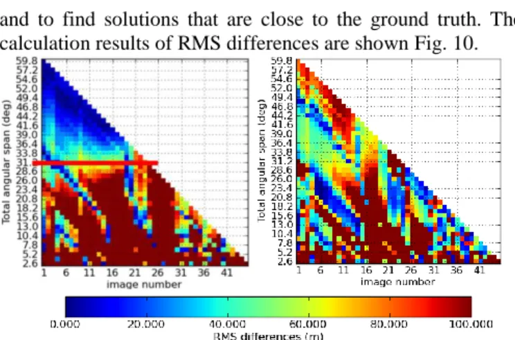
We first focus on Istres data and on the moving target presented in Fig. 8. We applied the inversion algorithm to calculate the moving target trajectory and to compare it to the GPS truth. Fig. 9 shows the RMS differences between the estimated trajectory of the real moving target on Istres data and its GPS position. The axis represents the index of the first image used to solve the system. Since the sensor is moving along the circular trajectory, this number is linked with the difference of orientation between sensor velocity and target velocity. The axis represents . We tested again the two different moving target models: the one with constant velocity (see Fig. 9, left) and the one with constant acceleration (see Fig. 9, right). As the real trajectory is not a trajectory with a perfect constant acceleration, the results are disturbed, depending on the images used to solve the system. These results show that from a certain angular span (corresponding to , see Fig. 9), the estimated trajectory is close to the GPS truth when we use a constant velocity model. It is not the case if we add the acceleration as a degree of freedom, which confirms the results of the PCA of the system (see Fig. 6 and Table II).
Another way to encompass the instability responses of the constant acceleration model is to add an orientation constrain given by the road network [25]. The addition of the road orientation thus allows to reduce the computation time 0.1 10 0 50 100 150 200 Par tial In e rtia (% ) Angular span (°) s1 s2 s3 s4
and to find solutions that are close to the ground truth. The calculation results of RMS differences are shown Fig. 10.
Fig. 9: RMS differences between the estimated trajectory of a real moving target around the city of Istres and its ground truth (GPS data). On the left is the result with the constant velocity model and on the right is the result with the constant acceleration model. The red line on the left represent the angular span at which the trajectory estimation is close to the GPS truth.
These results are obtained using the moving target model with constant acceleration. In this case, 3 different directions are proposed to the system. The method automatically selects the orientation that minimizes ( ) given by (13). We can see that in most cases, the estimated trajectory corresponds to the GPS truth.
Fig. 10: RMS between the estimated trajectory of a real moving target around the city of Istres and its ground truth (GPS data), with a model containing an information about the road network.
These results show that if we use the road directions (in urban context), the trajectory estimation is very precise, even with small angular spans. As the results are obtained with the constant acceleration model, the trajectory reconstruction method is efficient for more complex movements. If the road network is not used, we have to choose the moving target model with constant velocity and a large enough angular span to retrieve precisely the moving target trajectory. It induces a tradeoff between the angular span, the precision of the reconstruction and the constant velocity hypothesis.
One of the configurations of Fig. 9 is used to show an example of trajectory reconstruction of the moving target (see Fig. 11). We took a time interval between the two farthest images equal to (corresponding to a total angular span equal to approximately) to calculate this trajectory. The red dots represent the result of the trajectory computation and the green dots represent the apparent trajectory of the moving target. We then compare the result of the calculation with the GPS data and we compute the RMS differences between the result of the trajectory computation and the GPS data (the results are listed in the table IV).
The moving target trajectory reconstruction is very accurate. The average position RMS error on the whole target trajectory is less than . The error of the velocity is , which correspond to an average error about 2%. Concerning the acceleration and orientation errors, they are very low ( and , respectively).
Fig. 11: trajectory reconstruction for a real known trajectory (with ground truth) near the Istres airport. The red dots represent the result of the trajectory computation, and the green dots represent the apparent trajectory of the moving target. The moving target is a Renault Master travelling at an average speed of .
TABLEIV
RMS DIFFERENCES BETWEEN THE RESULT OF THE TRAJECTORY COMPUTATION AND THE GROUND TRUTH (GPS DATA) AROUND THE CITY OF ISTRES
Symbol Quantity Value
Ground position RMS differences Velocity RMS differences Acceleration RMS differences Orientation RMS differences
Fig. 12 shows the trajectory of the moving target obtained around the city of Nîmes concerning the moving target with unknown movements. We took a time interval between the two farthest images equal to (corresponding to a total angular span equal to approximately) to calculate this trajectory.
Fig. 12: trajectory reconstruction for a real unknown trajectory. Red circle is the train station of the city of Nîmes. The red dots represent the result of the trajectory computation, and the green dots represent the apparent trajectory of the moving target. The green (dotted) line represents the railway.
The moving target model used for calculation is a constant velocity model. The green dots represent the apparent trajectory of the moving target during the time , i. e. the coordinates of the moving target centre in all the SAR images used for the trajectory calculation. The coordinates of the moving target centre is obtained by using the measurement methodology described on the section II. We projected all
these coordinates on a single image for visualising. We can see the apparent position of the moving target on the image shown here in the yellow rectangle. The measured velocity of the moving target is almost constant and equal to . Furthermore, the target is very close to the railway (green dotted lines). The result of the trajectory computation is shown in the white circle (red dots). All these characteristics are consistent with a train arrival in the Nîmes station (red circle).
V. CONCLUSION
This paper presents a novel methodology to track moving target from the apparent coordinates of the moving targets in a set of SAR images acquired along a circular trajectory in monosensor spotlight mode. This method consists in inverting a equation system, being the number of used images. The apparent coordinates measurements are given by an autofocus and relocation method. A validation with synthetic aircraft and target trajectories was carried out, testing two different moving target models: one with a constant velocity and one with a constant acceleration. The computation of the RMS differences between the estimated trajectory and the synthetic ground truth combined with a mathematical analysis of the system has highlighted the sensitivity of the method when we consider the moving target acceleration and its stability with the constant velocity model.
Some results concerning real moving targets trajectory reconstruction are shown around the city of Istres and Nîmes. The computation of the RMS differences confirms the results on synthetic trajectories and proved the efficiency of the method with the constant velocity model and from a certain angular span. Concerning Istres data, we examine a moving target with ground truth (GPS data), and the comparison between the estimated trajectory and the GPS data gives position RMS differences of less than meters. For Nîmes data, the results concern a moving target which is supposed to be a train and the inversion method gives a trajectory which is close to the railway.
Another way to encompass the instabilities using the constant acceleration model is to add an orientation constrain given by the road network. With these constrains, we obtain effective results in almost all cases. Further studies could be done following this work. For example, the impacts of the azimuth resolution on the validity of the second order phase history of the moving target. Indeed, a good azimuth resolution is linked to a large integration time, and in this case, high order terms in the phase history cannot be neglected. The impacts of these terms have been studied in a multisensor context [8] but not yet in a circular monosensor case. The contribution of a second antenna can also be discussed, especially if the acceleration of the moving target is taken into account.
ACKNOWLEDGMENT
The authors would like to thank the RAMSES NG team (O. Ruault du Plessis, R. Baqué, G. Bonin, P. Fromage, and D. Heuzé) for having acquired the data around the city of Istres, the pilots for having performed the circular path.
REFERENCES
[1] I. G. Cumming and F. H. Wong, Digital Processing of Synthetic
Aperture Radar Data, Algorithms and Implementation. Boston, MA:
Artech House, 2005.
[2] R. K. Raney, “Synthetic aperture imaging radar and moving targets,”
IEEE Trans. Aerosp. Electron. Syst., vol. AES-7, no. 3, pp. 499-505,
May 1971.
[3] G. Wang, X-G. Xia, V. C. Chen and R. L. Fielder, “Detection, location and imaging of fast moving targets using multifrequency antenna array SAR,” IEEE Trans. Aerosp. Electron. Syst., vol. 40, no. 1, pp. 345-3555, Jan. 2004.
[4] J. Ward, Space-time adaptive processing for airborne radar . M IT Linc oln Lab., Lexin gt on, M A, Tech. R ep. 1015, Dec. 1994. [5] A. Budillon, V. Pascazio, and G. Schirinzi, “Estimation of radial velocity
of moving targets by along-track interferometric SAR systems,” IEEE
Geosci. Remote Sens. Lett, vol. 5, no. 3, pp. 349-353, Jul. 2008.
[6] M. I. Pettersson, “Optimum relative speed discretization for detection of moving objects in wide band SAR,” IET Radar, Sonar Navig., vol. 1, no. 3, pp.539-553, Mar. 2007.
[7] S. R. J. Axelsson, “Position correction of moving targets in SAR imagery,” Proc. SPIE, vol. 5236, pp. 80-92, Jan. 2004.
[8] J. J. Sharma, C. H. Gierull, and M. J. Collins, “The influence of target acceleration on velocity estimation in dual-channel SAR-GMTI,” IEEE
Trans. Geosci. Remote Sens., vol. 44, no. 1, pp. 134-147, Jan. 2006.
[9] G. Bonin and P. Dreuillet, “The airborne SAR system SETHI: Airborne microwave remote sensing imaging system,” in Proc. EUSAR, Friedrichshafen, Germany, 2008, pp. 1-4.
[10] R. Baqué and P. Dreuillet, “The airborne SAR-system : RAMSES NG Airborne microwave remote sensing imaging system,” in IET
International Conference on Radar Systems (Radar 2012), Glasgow, UK,
2012, pp. 1-4.
[11] J. R. Fienup, “Detecting moving targets in SAR imagery by focusing,”
IEEE Trans. Aerosp. Electron. Syst., vol. 37, no. 3, pp. 794-809, Jul.
2001.
[12] T. Sparr, “Time-frequency signature of a moving target in SAR images,” in Proc. RTO-MAP-SET, 2004, pp. 1-8.
[13] R. P. Perry, R. C. Dipietro and R. L. Fante, “SAR imaging of moving targets,” IEEE Trans. Aerosp. Electron. Syst., vol. 35, no. 1, pp. 188-200, Jan. 1999.
[14] P. A. C. Marques and J. M. B. Dias, “Velocity estimation of fast moving targets using a single SAR sensor,” IEEE Trans. Aerosp. Electron. Syst., vol. 41, no. 1, pp. 75-89, Jan. 2005.
[15] V. C. Chen, “Time-frequency analysis of SAR image with ground moving targets,” Proc. SPIE, vol. 3391, pp. 295-302, Apr. 1998. [16] M. Kirscht, “Detection and imaging of arbitrarily moving targets with
single-channel SAR,” Proc. Inst. Elect. Eng.-Radar Sonar Navig., vol. 150, no. 1, pp. 7-11, Feb. 2003.
[17] K. Ouchi, “On the multilook images of moving targets by Synthetic Aperture Radars,”IEEE Trans. Antenn. Propagat., vol. 3, no. 8, pp. 823-827, Aug. 1985.
[18] M. Kirscht, “Detection and focused imaging of moving objects evaluating a sequence of single-look SAR images,” in Proc. 3rd Int. Airborne Remote Sens. Conf. Exhib., Copenhagen, Denmark, Jul. 1997, vol. I, pp. 393-400
[19] J. M. B. Dias and P. A. C. Marques, “Multiple moving targets detection and trajectory parameters estimation using a single SAR sensor,” IEEE
Trans. Aerosp. Electron. Syst., vol. 39, no. 2, pp. 604-624, Apr. 2003.
[20] M. Soumekh, “Reconaissance with slant plane circular SAR imaging,”
IEEE Trans. Image Process., vol. 5, no. 8, pp. 1252-1265, Aug. 1996.
[21] L. Perlovsky, R. Ilin, R. Deming, R. Linehan and F. Lin, “Moving target detection and characterization with circular SAR,” in IEEE Radar
Conference, Washington, DC, 2010, pp. 661-666.
[22] J.B. Poisson, H. Oriot, F. Tupin, “Performances analysis of moving target tracking in circular SAR,” in Proc. IRS, Dresden, Germany, 2013, pp. 1-6.
[23] J. B. Poisson, H. Oriot, F. Tupin, “Moving target tracking using circular SAR imagery,” in Proc. EUSAR, Nuremberg, Germany, 2012, pp. 1-4. [24] J. A. Fessler, “Moments of implicity defined estimators (e.g., ML and
MAP): Applications to transmission tomography,” Proc. Int. Conf.
Acoustics, Speech, and Signal Processing, vol. 3662, pp. 2291-2294,
1995.
[25] P. A. C. Marques, “SAR-MTI improvement using a-priori knowledge of the road network,” in Proc. Eur. Radar Conf., Oct. 2010, pp. 244-247.