HAL Id: hal-01890617
https://hal.archives-ouvertes.fr/hal-01890617
Submitted on 4 Nov 2020
HAL is a multi-disciplinary open access
archive for the deposit and dissemination of
sci-entific research documents, whether they are
pub-lished or not. The documents may come from
teaching and research institutions in France or
abroad, or from public or private research centers.
L’archive ouverte pluridisciplinaire HAL, est
destinée au dépôt et à la diffusion de documents
scientifiques de niveau recherche, publiés ou non,
émanant des établissements d’enseignement et de
recherche français ou étrangers, des laboratoires
publics ou privés.
Residence time distribution on flow characterisation of
multichannel systems: Modelling and experimentation
Xiaofeng Guo, Yilin Fan, Lingai Luo
To cite this version:
Xiaofeng Guo, Yilin Fan, Lingai Luo. Residence time distribution on flow characterisation of
multi-channel systems: Modelling and experimentation. Experimental Thermal and Fluid Science, Elsevier,
2018, 99, pp.407 - 419. �10.1016/j.expthermflusci.2018.08.016�. �hal-01890617�
Contents lists available atScienceDirect
Experimental Thermal and Fluid Science
journal homepage:www.elsevier.com/locate/etfsResidence time distribution on
flow characterisation of multichannel
systems: Modelling and experimentation
Xiaofeng Guo
a,⁎, Yilin Fan
b, Lingai Luo
baESIEE Paris, Université Paris Est, LIED UMR CNRS 8236, 2 boulevard Blaise Pascal– Cité Descartes, 93162 Noisy Le Grand, France
bLaboratoire de Thermique et Energie de Nantes (LTEN), UMR CNRS 6607, Université de Nantes, Rue Christian Pauc, BP 50609, 44306 Nantes Cedex 03, France
A R T I C L E I N F O Keywords:
Residence Time Distribution (RTD) Non-intrusive measurement Flow distribution Multichannel device
A B S T R A C T
Residence Time Distribution (RTD) is a frequently used tool in conventional process equipment and it provides internalflow characterisation by simple tracer tests. In this paper, we explore the feasibility of using RTD to identifyfluid distribution uniformity in millimetric multichannel devices. Both theoretical modelling and ex-perimental implementation are conducted to 16-channel systems. Theoretical modelling confirms the effec-tiveness of non-intrusive RTD measurements in evaluatingflowrate distribution uniformity. Different influencing factors, such as channel corrosion, blockage, distributor structure, channel length or width variation, etc., can be reflected by RTD response curve. The experimental setup consists of a lab-developed RTD test platform coupling a fast camera and two miniflowcells capable to quantify rapid tracer concentration evolution through carbon ink visualization. The platform is particularly powerful for very narrow RTD measurement with residence time down to 1 s. With the platform, we investigate the RTD characteristics of a multichannel device under severalflow conditions. Model correlation of the experimental data gives valuable information such asfluid distribution, plug-flow ratio and perfectly mixed volume.
1. Introduction
Significant progresses in Process Intensification [1,2] have been seen in last decades. They are characterised by compact size and en-hanced performances influids mixing, heat transfer as well as chemical syntheses yields. However, industrial applications usually require large production rate which in general means high throughput, a weak point for most micro- or mini-devices. Numbering-up process[3–8]is then applied, in the form of 2D or 3D multichannel/layer systems or modular reconfigurable devices. Particularly for multichannel systems, the par-allelisation of a large number of flow/mixing/reaction paths helps achieve industrial-level production.
Fluid distribution uniformity in multichannel devices is considered as a key issue to achieve high global performances. A number of studies in the literature have confirmed the influence of flowrate distribution in multichannel heat exchangers [9], mixers[10,11] and chemical re-actors[12–14]. One of the existing difficulties in the evaluation of fluid distribution influence lies in the identification of flow distribution uniformity (in terms offlowrate). Non-intrusive measurements are ne-cessary in case of non-transparent devices for whichflow visualisation test is not applicable. This paper introduces our modelling and ex-perimentation works on the development of a non-intrusive method
based on Residence Time Distribution (RTD) characterization and its application to multichannel devices for their fluid flow distribution diagnostic.
1.1. Previous studies
Parallel millimetric channels can be configured to provide multiple functionalities including heat exchange, mixing and chemical reaction. Our previous studies[10,15,16]on a 16-channel device have demon-strated rapid mixing effect (with micromixing time down to 10 ms) and compact heat exchange property (with the overall heat transfer coef-ficient being in the range of 2000–5000 W m−2K−1). All these
perfor-mances are thanks to a special tree-like structure that serves asfluid distributor and collector. By using such a nature-inspired manifold, the flow distribution non-uniformity is estimated to be lower than 10% under testflow conditions.
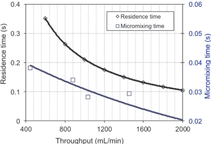
However, once channelflowrates differ among channels (non-uni-form distribution, or maldistribution), the global per(non-uni-formance is ex-pected to degrade in most cases. Regarding micromixing and chemical reaction, unevenfluid distribution can result in unbalanced reagents composition thus totally different reaction kinetics. Shown inFig. 1is the link betweenfluid residence time and micromixing time, previously
https://doi.org/10.1016/j.expthermflusci.2018.08.016
Received 3 December 2017; Received in revised form 9 July 2018; Accepted 13 August 2018
⁎Corresponding author at: ESIEE Paris, Department SEN, 2 bd Blaise Pascal BP99, 93162, Noisy Le Grand Cedex, France.
E-mail address:[email protected](X. Guo). Available online 15 August 2018
0894-1777/ © 2018 Elsevier Inc. All rights reserved.
measured inside the 16-channel device [16]. It can be seen that, without a mechanical aided mixing, the two time variables are closely related and dependent on the channelflowrate. In other words, uneven flowrate distribution in a multichannel device may result in different micromixing time among channels, implying less controllable syntheses and heterogeneousfinal products.
In some specific cases, uneven fluid distribution may have positive influence on mixing. As in the study of Su et al. 2015[17]on a mul-tichannel zigzag microreactor, if the overallflowrate is kept the same, partial channel blockage may enhance mixing since more fluid per-turbation happens in non-blocked channels with higherflowrates. In case of gross maldistribution, strongerfluid impingements in collectors also enhance the mixing process. However, the above conclusions only are applicable only under two conditions: (i) the mixing should be slow so that it does notfinish before going into the collector zone, and (ii) a higher pressure loss with the same overall flowrate guaranteed by a pump. Our study focuses on straight pipes that will be used for rapid mixing/reaction applications and we suppose that they all require uniformfluid distribution for better performance.
As the influence of flow distribution uniformity on various perfor-mances of multichannel device is significant, the perfect reproduction of single pipe performances is strongly expected during numbering-up process. The ability to predict or identify the fluid distribution uni-formity in a multichannel device by a non-intrusive experimental method is hence helpful.
1.2. Existing methods influid distribution identification
Main methodologies in the diagnostic offluid distribution in mul-tichannel devices can be categorized by numerical simulation andflow visualization. The use of non-intrusive tool such as RTD should be much helpful yet not sufficiently advanced in the literature.
CFD (Computational Fluid Dynamics) simulation is an interesting and practical tool intensively used for the prediction or characterization of hydrodynamic and/or thermal properties of multichannel devices, sometimes with the purpose of structural optimization. A number of studies using CFD tools have been reported in the literature[18–21]. Nevertheless, it should be noted that current CFD techniques still have some difficulties in correctly describing turbulent flows, vortex or curvatureflows and multi-phase flows. Moreover, CFD results need to be validated by experimental measurements.
Besides numerical methods, existing experimental techniques for the evaluation of fluid distribution are limited to visualizations by color, pH indicator or fluorescence tracers [22–24]. Other intrusive experimental methods such as Hot Wire Probe (HWP), Doppler Ultra-sonic Velocimetry (DUV) are compared by Boutin et al.[25]. But the
above-listed techniques give only single point measurement other than detailed flow distribution information. Concentration measurement using salt as tracer[26]can be an effective solution for conventional devices. When comes to millimetric device that have short residence time, this method is limited by the sampling rate of conductometer. PIV (Particle Image Velocimetry)[25,27]and LIF (Laser Induced Fluores-cence) [28]measurements provide quantitative velocity distribution inside certainflow configurations, but under specific conditions. First, the visualization is usually limited to simple or single-pipe devices but not adapted to 3D complex configurations. Second, PIV or LIF mea-surements require that the studied structure being transparent[28]in accordance with the wave length of the laser source.
The development of a non-intrusive tool for fluid distribution characterization based on inlet-outlet detection should be more prac-tical for the identification of general multichannel flow systems. To the authors’ knowledge, very few studies in the literature addressed the fluid distribution issue by RTD tool. Detailed RTD analyses merit being involved to explore the relationship between RTD characters and the flow distribution uniformity.
1.3. RTD and its application
Non-intrusive tracer test has been widely used in process en-gineering except for quantitativefluid distribution determination. After the pioneer work of MacMullin and Weber in 1935[29]and several classical interpretations of RTD by Danckwerts in 1953[30], extensive applications have been found in the field of chemical engineering. Macro-mixing and hydraulic characteristics of a process device could be reflected through examining the RTD curve [31]. RTD has also been used to predict the chemical reaction conversions by combining che-mical kinetics and RTD analysis[32]or to determine optimal design parameters of tubular reactors[33]. Besides conventional RTD models for CSTRs (Continuous Stirred Tank Reactor) and PFRs (Plug Flow Reactor), some recent applications in multichannel systems in the aim of flow and mixing characterisation attracts some attention too [34–38]. In particular, recent works by Wibel et al.[39]investigated the impact of inlet/outlet volumes and unevenflow distribution on the RTD characters of micro devices consisting of an array of parallel mi-crochannel, by both CFD simulation and experimental characterization. For miniaturized process devices, one of the challenges to conduct a RTD analysis lies in the choice of tracer and its detection instrument. Especially for non-transparent devices, particle or dye visualisation [40] are generally impossible. Dong et al. [41] developed single channel Ultrasonic Microreactor and studied the effect of ultrasonic field on the mixing and RTD. The mechanism of ultrasonic induced cavitation (bubbles sizing 100–200 µm) intensifies radial mixing and reduces axial dispersion within the reactor channel (characteristic di-mension from 250 µm to 1 mm). Their RTD measurements are based on UV–Vis spectrometer tracing 5 g/L uranine solution. This technique is more adapted to long residence time (around 100 s in their case). For very narrow RTD measurement, the spectrometer’s sampling time may limit its application. In conclusion, quantitativefluid distribution (in terms offlowrate) determination by an easy-to-use RTD measurement is still lacking. Moreover, due to short residence time and narrow RTD curve of millimetric devices, traditional methods like conductivity measurement using salt as tracer [26], become limited by sampling rates. Developing a rapid RTD detection platform applicable to micro-or mini-fluidic devices is then of practical significance.
1.4. Current study
The main contribution of this study is to demonstrate the utility of RTD tool for the characterization of fluid distribution uniformity in multichannel devices. The study begins with the modelling of the RTD behavior of multichannel device with non-uniform distribution as-sumptions; then, an experimental platform applied to a previously
0.02 0.03 0.04 0.05 0.06 0 0.1 0.2 0.3 0.4 1200 400 800 1600 2000 Micromixing time (s) Residence time (s) Throughput (mL/min) Residence time Micromixing time
Fig. 1. The link between residence time and micromixing time in a static mi-cromixer.
developed mini-reactor is explained in detail.
The modelling and experimentation are conducted taking a 16-channelfluidic system as example. In the modelling part, axial disper-sion RTD representation isfirstly established in each channel, according to its flowrate and other geometrical parameters. Then, supposing flowrate deviation among the 16 channels, we obtain the global RTD of the whole device. The comparison between a perfect, homogeneous distribution case and a non-uniform distribution case will confirm the feasibility offlow distribution diagnostic through a non-intrusive RTD injection-response measurement. For the experimentation part, a tracer injection-detection platform with the aim of identifying short residence time and narrow RTD curves is introduced and explained in detail. The basic principle is instantaneous tracer concentration determination by using fast camera and image analysis. We confirm the feasibility of using the developed platform to identify the RTD of our device with throughput time down to 1 s. In general, this tracer test platform can be easily adapted to other micro- or mini-fluidic systems regardless of its residence time being long or short.
It worth noting that the modelling and experimental parts are not meant for results validation but to show independently the role of RTD study for distribution uniformity. We aim to show large RTD deviation due to unevenfluid distribution by making specific assumptions in the modelling process. The distributor and collector parts are not con-sidered in the model. In the experimental part, however, we use our previously developed reactor whose fluid distribution uniformity is already guaranteed thanks to tree-like bifurcation distributor and col-lectors.
The rest of the paper is organized as follows: (i) the RTD modelling of multichannelfluid system, (ii) detail of the development of a rapid RTD measurement system, and (iii) discussions on the overall metho-dology.
2. RTD modelling of a multichannel system
The procedure of the RTD modelling is as follows: (i) single pipe flow modelling under fully developed laminar condition using Dispersive Plug Flow (DPF) model; (ii) determination of flowrates in each channel in a multichannel device under different conditions, and (iii) composition of all single channel RTD signals to obtain the global RTD curve. Non-uniform flow distribution originated from different factors (channel length variation, width difference, distributor/col-lector design, etc.) is considered. The influence of channel flowrate deviation on the global RTD curve is modelled. However, fluid dis-tribution and collection are not considered in the model.
Pipe dispersiveflow is considered to model each channel before constructing the global RTD model for a multichannel system. The following general hypotheses are used:
(i) Fully developed laminarflow;
(ii) Circular cross section channels, pipeflow;
(iii) Only spatial dispersion (shear force induced diffusion) caused by velocity gradient (hence concentration gradient) is considered, turbulence caused diffusion does not exist.
2.1. Multichannel RTD modelling– general approach
In a multichannel system, the tracer concentration evolution under fully developed laminar flow in channel i can be expressed by DPF model, given by Eq. (1)[37]. The single channel RTD is a function of Peclet number Pe and dimensionless time t/τm.
⎜ ⎟ = + ⎛ ⎝ − + − ⎞ ⎠ E t Pe π t τ Pe t τ t τ ( ) 1 4 ( / ) exp ( 1)(1 / ) 4 / i i m i i m i m i , 3 , 2 , (1)
where Ei(t) represents the RTD response in channel i, t time of pipeflow
(s) andτmthe mean pass-through time (s).
The dimensionless Pe number is given by: =
Pe uL
D (2)
where u is the average velocity inside pipe (m s−1), L length of the pipe (m) and D the dispersion coefficient, (m2s−1), obtained with Taylor
correlation[31]: = + D D u d D m m 2 2 (3) Dmis the molecular diffusion of water, u the velocity of flow and d the channel diameter. In our case, the molecular diffusion is negligible compared with the axial dispersion.
Then the global RTD could be calculated using Eq. (4), by com-bining all individual RTD curves considering individual channel flow-rates as a weighting factor.
∑
= = E t Q Q E t ( ) 1 ( ) i n i i 1 (4)where Q is the total volumeflowrate, and Qi the individual volume
flowrate in channel i.
In a single pipe, hydraulic relation associates parameters including pressure loss (ΔPi), geometry (d and L) and flowrate (Qi), using
=
P f d L Q
Δi ( ,i i, i). Under laminar regime, the pressure loss for pipeflow is governed by Hagen-Poiseuille law given by Eq. (5). The equation, applied to different channels, provides basic calculation for flowrate distribution among different channels.
=
P μL Q
πd
Δi 128 i i
i4 (5)
Until this step, a RTD analysis can be constructed to a multichannel device, taking into account different cases such as channel length var-iation, diameter difference, gross fluid maldistribution due to dis-tributor design, block of one or several channels, corrosion of one or several channels, etc.
2.2. Flowrate distribution coupling
Based on the multichannel RTD model, two categories of cases are studied. The first category is passage-to-passage maldistribution, in-duced by variation of length, diameter, corrosion or blockage. The inlet distributor and the outlet collector are supposed to be perfect so that they provide equal pressure loss (ΔPi) to every channel. The second
category is named gross maldistribution case due to improper dis-tributor/collector design. In this case, channel geometric parameters including diameter and length are identical. However, the channel flowrate may differ from one pipe to another.
The two categories will be treated separately. For the passage-to-passage maldistribution category, the channelflowrates are calculated based on the pressure balance while for the gross maldistribution ca-tegory, theflowrate distribution is predefined. Once individual flow-rates obtained, the global RTD model is constructed by combining all individual RTD curves.
2.2.1. Case of length variation
Modelling of length-varied multichannel RTD is based on the fol-lowing hypotheses:
(i) Varied channel lengths Li;
(ii) Fixed total flowrate Q, internal volume V as well as identical channel diameter d;
= = = = = ∑ = P P P P P Q Δ Δ ... Δ Δ Δ i μ πd 1 2 128 i n Li 4 1 1 (6) (iv) Based on the previously determined pressure loss, individual
channelflowrate (Qi) is calculated as:
= Q πd μL P 128 Δ i i 4 (7) (v) Tracer (Dirac impulse) amounts injected into channels are
propor-tional toflowrate (Qi/Q);
The model assumptions with the length-varied geometry are illu-strated inFig. 2. Practically, the variance of channel length Liis usually
a result of impropriate design or imprecise fabrication of one or several channels during numbering-up process.
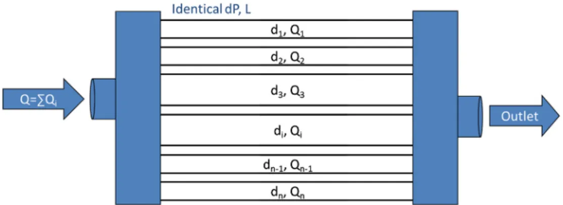
2.2.2. Case of diameter variation
In this case, all other hypotheses are the same as the previous one (Section 2.2.1), except for thefirst two:
(i) Varied diameter di, identical channel length L;
(ii) Fixed totalflowrate Q, and volume V;
Eqs. (6) and (7) in this case shall be modified as Eq. (8) for the determination of pressure loss and then Eq. (9) to obtain individual channelflowrate: = ∑ = P Lμ π d Q Δ 128 i n i 1 4 (8) = Q πd μL P 128 Δ i i 4 (9) The model assumptions with diameter varied geometry are illu-strated inFig. 3. Under practical situations, the variation of diameter di
may come from (i) total blockage of one or several channels; (ii) de-terioration enlarging the diameter; (iii) partial blockage of channel because of fouling; and (iv) impropriate design or fabrication of mul-tiple channels during the numbering-up process. It worth noting that in the total blockage situation, the model considers reduced number of channels and keeps the same pressure drop in the effective channels. 2.2.3. Case of gross maldistribution
The gross maldistribution is mainly due to improper design of dis-tributor/collector and one of them is the ladder network as shown in
the upper left corner ofFig. 4. The modelling process is based on hy-potheses below:
(i) Identical d and L for all pipes; (ii) Fixed Q, V;
(iii) Channelflowrate Qiis predefined in the following modelling;
(iv) Channel pressure loss (ΔPi) is no longer identical;
(v) Tracer (Dirac impulse) amounts injected into channels are pro-portional toflowrate (Qi/Q);
2.3. Results and discussion
The modelling is implemented in Matlab©[42]environment. The following discussions are based on both qualitative comparisons and quantitative statistical analyses. Under non-uniformflow distribution situation, individual RTD curves in pipe i might vary from one to an-other. After being put together, the shape and spreading character of the global RTD curve can be observed, which clearly differ from that under uniform distribution condition. Time location of concentration peak can be different too. Moreover, comparison of curve variance (σ2
) gives quantitative deviation information between non-uniform and uniform distribution conditions.
2.3.1. Case of length variation
Thefirst case study is a 16-channel system with identical diameter of 1 mm, but length varied from 0.44 to 1.94 m, following a parabolic curve as shown inFig. 5(a). The case of identical length of 1 m, which represents the same total volume (channel only, 12.6 mL) as the varied one, is also modelled for comparison. The pass-through time for both cases is the same, i.e., 12.6 s under aflowrate of 60 mL·min−1.
Shown inFig. 5(b) are RTD curves in all 16 channels for the varied-length case. For channels numbering from 5 to 11, their concentration peaks arrive within 10 s. The RTD peaks in longer channels, however, appear much later than the average pass-through time 12.5 s. Corre-sponding Pe number ranges from 2.3 for shortest channels in the middle to 17.1 for longest ones at the side.
The global inlet-outlet RTD curve, both in cases of varied- and identical length, are shown inFig. 5(c). Two features can be observed in thisfigure: the peak arrival time and the tailing effect. Firstly, it can be observed that under uneven distribution case, peak concentration ar-rives at around 2.5 s. Compared with the value of 6.5 s for identical channel case, the varied-length concentration peak arrives much ear-lier. A large number of tracers follows higherflowrates in short chan-nels. Secondly, length-varied multichannel device holds a tailing effect. The outlet tracer detection can last much longer than the average pass-through time; while for the uniform distribution case, no tracer can be detected after 30 s. This can be explained by much lower Pe number in
longer channels where tracers spend more time to traverse such paths. To quantitatively evaluate influence of length variation on the spreading character of RTD curve, the second moment of tracer curve, the variance (σ2), is analysed. Shown inFig. 5(d) are RTD curves of
multichannel device, with different degree of flowrate deviation (Qdv)
due to length variation. Note that the parameter Qdv, as shown in Eq.
(10), is defined as the maximal difference of flowrate among channels devised by the averageflowrate, [–]:A Qdvvalue of zero means perfect
distribution. = − Q Q Q Q dv i max i min mean , , (10) We may observe from the RTD curves that the higher theflowrate deviation (Qdv), the higher the order of magnitude of the RTD variance
(σ2). For the worst case, i.e.,flowrate deviation of 78% corresponds to a
variance of 120 s2in E(t) curve. While for the ideal uniform case, the
minimum value of variance is 38 s2. RTD is quantitatively shown to be more expanded with existence of distribution non-uniformity, meaning that the residence times for different portions of reactants are largely varied.
Absolute value of variance, however, depends highly on theflow conditions as flowrate, channel number, etc. Once the above para-meters arefixed, the variance of ideal RTD curve is fixed. Further RTD tests under the same condition, if showing a higher variance, means the departure from the uniform condition.
2.3.2. Case of diameter variation
In case of one or several channels being blocked or enlarged due to corrosion, the modelling considers diameter variation. The total volume V reduces while the globalflowrate Q is kept the same by a pumping system.
Shown in Fig. 6(a) is the comparison of obtained E(t) curves
between a case of 4 channels in 16 being blocked and another case without blockage. Frist of all, earlier tracer peaks at the outlet can be observed in the blockage case (3 s instead of 6 s). This means shorter pass-through time in case of channel blockage since part of the total volume becomes dead volume. Secondly, in contrary with the length variation case, no tailing effect is observed when 4 channels are blocked. Pelect number is increased due to dead volume and theflow becomes closer to pistonflow.
Simplified corrosion case can also be modeled by supposing en-larged diameter to one or several channels.Fig. 6(b) shows two RTD curves comparing in one case 20% enlarged diameter for 4 channels and the other under normal situation. The 4 enlarged channels result in expanded E(t) curve, meaning different Pe numbers in normal and en-larged channels. More precisely, extra volume in corroded channels results in smaller Pe number thus more diffusive flow. The global RTD curve in this case is then more expanded than a pistonflow.
2.3.3. Reflect of gross maldistribution by RTD
When it comes to the case of improper distributor or collector de-sign, the RTD curve can also be influenced by gross maldistribution. Flowrate in each pipe is imposed by a preset value according to uniform or non-uniform distribution case, as shown inFig. 7. Such parabolic distribution shape may be observed in typical Z-type ladder networks having one inlet pipe and one outlet pipe in diagonal position and perpendicular parallel pipes[43]. The total volumetricflowrate is kept at 60 mL/min, the same value as in Sections 2.3.1 and 2.3.2.
As shown inFig. 7(a) and (b), RTD curves under aflowrate devia-tion condidevia-tion can differ from those under uniform distribudevia-tion condi-tion. The difference can be slight (for the case of 10% deviated flowrate, (a) but becomes very distinctive when theflowrate deviation Qdv
in-creases (b).
For channels with high flowrate (at two sides as shown in the
Fig. 3. Multi-channel RTD model, case of diameter variation.
figures), tracer peaks appear much earlier than other channels, in-dicating shorter average residence time. Moreover, if we examine the spreading character of the RTD curves, wefind that uniform distribu-tion curve is less stretched compared with that withfluid deviation. Pe number in these channels is higher andflow is closer to plug flow.
The influence of maldistribution on RTD depends highly on flow-rates. At low flowrate, the influences are easier to be distinguished compared with highflowrates. In other words, the distribution issue at lowflowrate has more influence on the global RTD curve and may re-sult in more serious performance deterioration.
Fig. 5. Global and individual RTD curves for length varied non-uniform distribution cases.
2.3.4. Discussion
Other case studies were also performed, covering different channel numbers, different total flowrates or different Qdvvariations. Although
the shapes of global RTD curves and the correspondingσ2values may
vary case by case, the general trend is similar as the cases presented above. A global RTD curve appearing stretched or distorted (longer tailing, multiple peaks, etc.) with higherσ2value usually implies the
presence of unevenflow distribution.
In all cases of non-uniform distribution, the inhomogeneity of re-sidence time may degrade the global performance. For example as shown inFig. 5, peak concentration in the varied length case arrives at 2.5 s instead of 6.5 s for identical length case. This information can be obtained by RTD tests and thus shows as an effective internal flow identification tool. Regarding heat transfer, local heat transfer coeffi-cient depends on individual channel velocity (flowrate). The above RTD modelling results show how important a uniform fluid distribution should be kept in multichannel devices. The use of some optimised structures such as tree-like distributor[10],flat constructal distributor/ collector [7,17], etc., may help providing evenfluid distribution to avoid the above issue.
The analyses of the three maldistribution cases confirm the feasi-bility of reflecting fluid distribution characters by RTD test, instead of currently used visualisation or numerical methods. The next part fo-cuses on the development and implementation of a tracer test platform on multichannel devices.
3. High-speed RTD measurement 3.1. RTD detection system
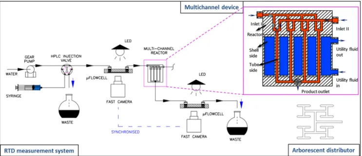
The high-speed tracer test platform is comprised of a high-speed camera, two lab-devised miniflowcells for ink observation, and an HPLC valve for tracer injection. Sampling time of this platform, which is critical for a short impulse response measurement, could be as short as 1 ms (1000 Hz) according to the frame-rates of the fast camera.
The test platform is described inFig. 8. One gear pump is used to circulatefluid through the 16-channel device. Here the device has two inlets and one outlet since it is initially designed to be multifunctional serving as both fluid mixers, heat exchangers and reactors. Details about the configuration can be found in our previous papers[10,15]. More specifically, the equal fluid distribution is confirmed being under 10% among the 16 channels. Tracer is injected to one of the inlets of device through using an HPLC valve, which is usually used for rapid injection of afixed volume of liquid. The other inlet was blocked during the RTD measurement. By doing this, both the fluid distribution,
collection and multichannel parts are investigated by RTD. Two mini-flowcells are placed shortly before the inlet and after the outlet of the multichannel device. The distance is kept as short as possible to avoid possible influence on the result. LED sources are employed to provide sufficient and adjustable luminance to the miniflowcells. Synchronised fast cameras are used to capture photos during the testing process. Water serves as the main circulationfluid through the multichannel device.
Carbon ink is chosen as the tracer in this test. Particles of carbon with sizes around 1 µm are dispersed homogeneously in water. By di-luting the inks into water in a trial-and-error manner, we realise an inversed grey scale change varying from 255 (white, no tracer detected) to the zero (black, most concentrated). In our case, we use an 8-bit image scale corresponding to a maximum grey scale of 255. Advantages of using inks are: (i) chemically stable; (ii) easy to be detected with monochrome fast camera; (iii) non-adhesive to pipe wall; (iv) en-vironment harmless; (v) negligible influence on the physical properties of liquid; etc.
As the key detection unit of this tracer test, two miniflowcells are designed and fabricated (Fig. 9) in laboratory. Basically, the mini-flowcell provides a narrow flow path of 0.5 mm for fluid so that light passed through the miniflowcell is inversely proportional to the con-centration of tracer. Photo sequences taken by fast camera every 1 ms then reflect different grey scales. Through image analyses and data normalisation, evolution of the tracer concentration with time is ob-tained.
As it is practically impossible to realise a real Dirac injection, short pulse input is generally used. For all test cases, the injection tracer volume isfixed at 15 µL by the HPLC 6-way valve.
3.2. Signal treatment
Image treatment and post analyses are implemented using an open source tool ImageJ[44]. Grey scales of captured image sequences with time stamp are analysed in a‘Batch’ manner, i.e. a large quantity of time-labelled photos are analysed in a single process. Concentration of tracers is then calculated with respect to time. Finally, inlet and outlet concentration curves are normalised so that the surface area under the curves equals 1.
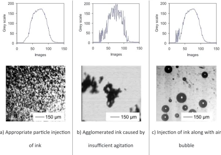
Several precautions should be taken before and during the experi-ments. First of all, the injection of tracers should be done after agitating the tracer solutions. Ink particles tend to agglomerate after being left still for several hours. The appearance of ink particle agglomerations (shown inFig. 10b) may influence the continuity of measurement, thus the accuracy on the concentration. Special attention should be given
during the injection progress. Some air bubbles may enter the system when injecting the small volume of tracer by HPLC valve. This may also give noise to the measuring results (see Fig. 10c) and should be avoided. One way to prevent air from passing inside is to switch the valve in a very fast manner. Some researchers used electric solenoid or piezoelectric actuator to switch the valve as presented in the paper [45].
3.3. Post processing 3.3.1. Beer-Lambert law
The relationship between ink concentration and captured light in-tensity is exponential according to Beer-Lambert law:
= −
I I e ε lC
0 ink (11)
where I stands for the light intensity measured after the miniflowcell with ink-in-water as medium, and I0is that with pure water as medium;
εinkis the extinction coefficient of ink, L·mol−1·cm−1; l the optical path
of miniflowcell, cm; and C the concentration of ink in water, mol·L−1.
Withεinkand l being constants, an exponential relationship between
concentration and light intensity can relate images grey scale with concentration: ∝ = C I I G G ln 0 ln 0 (12) where G is the inversed grey scale of images, 0 to 255; G0= 255 is the
inversed grey scale value in the case of pure water. It worth noting that
the minimum value of measured G in our experiment is kept higher than 0, i.e., the darkest image is not fully opaque. This is to guarantee that even in case of the highest concentration, the grey scale is still under saturated.
Obtained concentration C should still be normalised so that the area under the concentration/time curve equals 1.
3.3.2. Noise elimination
Random noises could be eliminated by applying higher frequency noise removal. The simplest method is the moving average one, suitable for large deviated noise eliminating. Preset value of noise limit is ob-tained by trial-and-error. + − > + = − + if C n C n set value C n C n C n ( 1) ( ) _ ( 1) ( ( 1) ( )) 2 (13) 3.3.3. RTD modelfitting
Two theoretical RTD models may be used to approximately re-present theflow behaviour in the multichannel device: DPF model (Eq. (1)) and compartment model[31,37]. The later combines a PF portion and a fully mixed one (CSTR), by defining a volumetric plug flow proportionθP.
The compartment model considers part of the reactor volume being PF (P) and the other part being CSTR (M) and it can be expressed by:
Fig. 8. A tracer test platform and its working principle for a rapid residence time distribution characterisation of a multichannel device.
a) concept of the lab-developed miniflowcell
b) photo of the two miniflowcells
= ⎧ ⎨ ⎩ < − ⩾ −
(
− −)
E θ for θ θ for θ θ ( ) 0 exp P θ θ θ θ θ P 1 1 P 1 1 P P P (14)whereθ = t/τmis the dimensionless time,θP=τ τP m,τm=τP+τMand =
τ τP M V VP M, RTD E(t) of this model can be calculated with known mean residence timeτmand givenθP.
To approximatelyfit the measured response curve with one of the two theoretical RTD models, basic parameters are firstly pre-set. It concerns the Pe number for the case of DPF and plug flow volume proportionθPfor compartment PF-CSTR model. Then, RTD models are
obtained by using spatial pass-through time (τm,spatial) as the mean
re-sidence time. Next, RTD models are convoluted with experimental input signal to simulate a standard model response to the real injection. The difference between convoluted model response and tested response is minimized by adjusting Pe orθPby an iterative calculation.
Calculation of outlet concentration from inlet tracer concentration and E(t) is a forward problem and it involves a convolution process according to Eq. (15). Convolution tool of Matlab© is utilized for this procedure.
∫
= − ′ ′ ′ Cout( )t C (t t)· ( )E t dt t in 0 (15)Model predicted RTD is obtained by adjusting different parameters (Pe for DPF model andθPfor PF + CSTR model). In this step, the
cu-mulative deviation between convoluted response Cout,fitand measured
response Cout,testis integrated:
∫
= − = ∑ − ∞ = ∞ E C t C t dt C t C t t | ( ) ( )| | ( ) ( )| Δfit out fit i out test i
i
out fit i out test i
0 , ,
1
, ,
(16) During thefitting process, the Efitis minimized to identify the most
appropriate Pe and θP values. The defined cumulative error has a
maximum value of 1 since both Cinand Coutsignals are normalized. The
smaller this value, the closer the model convoluted response from measured response. Corresponding RTD expressions are then obtained.
3.3.4. Determination of mean residence time
Thefirst calculation of mean residence time is through the spatial circulating time offluid through studied volume:
=
τm spatial, V Q (17)
The other way of mean residence time determination is from the basics of RTD. After tracer tests, the mean residence time could be calculated by the difference between the average injection time and outlet time, subtracted by the time passing through the detecting miniflowcell: = − − = ∑ ∑ − ∑ ∑ − = = = = τ τ τ τ t C t C t t C t C t V Q ( ) ( ) ( ) ( ) /
m measured response inject flowcell i
n i out i i n out i i n i in i i n in i flowcell , 1 1 1 1 (18) The comparison of the two residence times helps verify the precision level of the measurement tool.
a) Appropriate particle injection
of ink
b) Agglomerated ink caused by
insufficient agitation
c) Injection of ink along with air
bubble
0 50 100 150 200 0 50 100 150 Images Gr e y s ca le 0 50 100 150 200 0 50 100 150 Images Gr e y s ca le 0 50 100 150 200 0 50 100 150 Images Gr e y s ca leFig. 10. Ink injection should be prepared with precaution and cases should be avoided like (b) agglomeration and (c) bubble presence; Obtained grey scale curves are shown above the images (Images captured through fast camera and miniflowcells, post processed through ImageJ).
3.4. Results and discussions
A series offive tests is implemented to the 16-channel device. Tests are carried out under stable state without any leakage or tracer ab-sorbance. Severalflowrate conditions are tested and their characteristic parameters including Re and spatial pass through time are shown in Table 1.
Regarding theflow regime, it worth noting that the tested reactor is a multichannel device with arborescent (tree-like) distributor and col-lector. Flowrates in different levels of the multi-scale structure differ so as to the corresponding Re number. For example in the case of R1, a totalflowrate of 280 mL·min−1gives a maximum Re of 2324 (transi-tional flow in the collector outlet), while that of channel Re is 185 (laminar). Therefore, different flow regimes co-exist in this multi-channel device, with multi-channelflow basically being laminar.
3.4.1. Tracer concentration curves
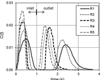
Curves of Injection and response in tested cases are shown in Fig. 11. Under different flowrate conditions, the injection and response concentration curves are clearly distinguished. As in the lowestflowrate case, i.e. R1, both inlet and outlet concentration curves last longer than the other tests. The expanded concentration is mainly due to the low volume flowrate imposed to R1. From R1 to R5, the inlet and outlet concentration durations decrease withflowrate augmentation.
The output concentration is more expanded than its corresponding input one, showing a dispersive character due to the internal multi-channel structure. For each of the five cases, the tracer is detected during longer time than its corresponding input signal. As the case of R5, its injected tracers become undetected starting from 0.6 s. On the other hand, the output tracers are observed starting from 1.1 s and disappear from the detection miniflowcell at 2.2 s. The pulse interval changes from 0.6 s at the inlet to 1.1 s at the outlet, meaning a sig-nificant dispersive mixing inside the heat exchanger reactor.
3.4.2. Precision verification by mean residence time
To examine the precision of the tracer test process, the measured residence time and the theoretical spatial pass-through time are plotted in Fig. 12. Both residence times follow an inversely proportional character withflowrate. In most cases, the two residence times are close to each other, except for that of the case R2 (325 mL·min−1). The average relative error is 7.2% and that of maximal error is 19.1% (case of R2). The reasons for uncertainties are twofold. First, instrumentation errors exist inflowrate determination and tracer concentration detec-tion. For example, the significantly deviated case R2, observed after repeated tests, is probably due to mechanical vibration resonance be-tween the pump and the tested device. Second and most probably, the complexflow characteristic of the studied device, including distribu-tion/16-channel/collection zones and each of them has different flow regimes, may give uncertainties. This will be discussed in the model fitting part.
3.4.3. Modelfitting results
Theoreticalfitted DPF and PF-CSTR RTD E(t) and E(θ) curves are shown inFigs. 13and14, along with identified Pe and θPvalues. Fitting
errors between experimental results and both models range from 10% to 22%, with the PF-CSTR model closer to the experimental results. These curves eliminate the imperfect impulse injection effect on the response, and they provide information such as residence time, plug flow degree, mixing volume fraction, etc.
First of all, as discussed earlier, the residence time shortens with increasingflowrate. For higher flowrates, the first detection of tracer arrives earlier and this can be observed both from the DPFfitted result and the PF-CSTR one.
Secondly, from the DPF results, the plugflow degree for all cases are very high with an identified value of Pe ranging from 168 (R5) to 317 (R3). In general, a Pe number higher than 100 is considered as a highly plugflow. This plug flow seems to be more distinguished for the case R3, with a Pe number of 317.
Finally, examining the parameterθPmay give information on the
proportion of mixing volume in the total volume. As the compartment model separates the reactor in two parts: a part of perfect mixing and the other perfect plugflow, it may be more adapted to our system in-cluding tree-like distributor/collector and 16 channels. ExperimentalθP
ranges between 0.87 (R5) and 0.91 (R3), indicating around 90% of the total volume being occupied by pure plugflow. Thus, only a small portion of volume in the reactor is used as mixing volume and in par-ticular in the tree-like split-and-combine structure.
Table 1
Summary offive RTD tests and their corresponding conditions. Test FlowrateQ (mL min−1) MaximumRe (–) ChannelRe (–) Thereotical pass-through timeτm(s) R1 280 2324 185 1.05 R2 325 2698 215 0.91 R3 400 3320 264 0.74 R4 440 3652 291 0.67 R5 493 4094 326 0.6
Fig. 11. Experimental RTD input and response through multichannel device, cases from R1 to R5, total flowrate increased from 280 mL min−1 (R1) to
493 mL min−1(R5).
Fig. 12. Comparison on theoretical pass-through time and detected mean re-sidence time, cases from R1 to R5, indicating an average error of 7.2%.
3.4.4. Discussion
The first conclusion by examining the RTD curves of the multi-channel device is on the fluid distribution uniformity. As discussed earlier in this paper,flowrate deviation among channels may give rise to distorted RTD curves such as higher variance, double peak in the response curve, etc. Since none of our test results (R1-R5) reflects a second peak,fluid distribution is thus considered to be relatively uni-form.
According to a correlation given by Levenspiel[31], for a DPFflow and with Pe higher than 1, the RTD curve variance is inversely pro-portional to Pe by: = σ Pe 2 θ2 (19) Fig. 15demonstrates the comparison between the theoretically and experimentally obtained relationship between Pe number and normal-ized variance. From thefigure, the test result is shown to hold the same trend as that given by theory. The difference in value is mainly due to the fitting deviation from original signal to model convolution. This comparison can also serve as a verification of the effectiveness of the developed RTD measuring system.
Earlier study [10]on the same multichannel device has revealed efficient mixing effect, both in macro scale and micro scale. It may be interesting to compare the low volume used for mixing from the RTD
tests. As discussed earlier, only 10% of the total volume has been used for species mixing. As a result, the mixing effect happens in a very local position in the reactor. The rest of the device, however, is characterised by highly plugflow.
a): E(t)
c
u
r
v
e
b E( ) curve
)
:
Fig. 13. RTD curves obtained by DPF modelfitting.a): E(t)
c
u
r
v
e
b E( ) curve
)
:
Fig. 14. RTD curves obtained by PF-CSTR modelfitting.
Fig. 15. RTD normalized variance with respect to Peclet number (DPF model fitting).
For such a multichannel complexflow system as studied, being high degree plugflow does not conflict with its efficient mixing character. On the contrary, a reactor with very local and efficient mixing, while with plug flow for the reaction functional part, is beneficial for un-dertaking chemical reactions. If comparing with a CSTR reactor, the advantage of current reactor is the local mixing effect instead of mixing in the global reactor size.
Finally, both DPF and PF-CSTR models can be implemented for the modelfitting and they give different information and precisions. The currently tested 16-channel system represents a relative short pipeflow (L/d = 50/2 cm), connected to a distributor and a collector. This con-figuration is more adapted to PF-CSTR model since it separates the volume into two zones. In the case of higher length/diameter ratios and without distributor/collector (e.g., the cases in the modelling part), the DPF model might be more adapted for thefitting process.
4. Conclusions
A RTD model for multichannel devices, considering diameter, length and distributor/collector induced flowrate variations is con-structed in this study. Different situations are analysed using the model and compared with that of perfectly uniform distribution situation.
Comparisons show how fluid distribution uniformity may be re-flected by global RTD curve. For example, compared with the case of even length distribution, a varied-length system will receive its peak concentration earlier, meaning a shorterfluid passage time for some channels. However, its tail could last much longer than that of uniform length case. Similar results can be obtained for the cases of channel blockage, corrosion, and gross maldistribution (due to distributor de-sign).
These results demonstrate that RTD can be a useful tool for the diagnostic offlow distribution non-uniformity. The identification of the above-mentioned problems in multichannel devices using non-intrusive tracer test is then possible.
An experimental platform is then constructed taking a 16-channel device as example. The ink-based tracer test platform, together with fast camera detection, is able to determine narrow RTD with mean re-sidence time as short as 600 ms. The RTD test shows a uniformflowrate distribution and quasi plug flow pattern (Pe > 168) in the tested multichannel device with no short-circuit, backflow or stagnant area observed. Together with its data processing procedure, the experiment platform can be used to characterize various millimetric multichannel devices with short or long pass-through time.
Our future efforts are emphasized on applying the above theoretical and experimental approaches to other type of multi-channel systems, with a special attention on the fluid distribution issue according to distributor design.
References
[1] A. Stankiewicz, J.A. Moulijn, Process intensification: transforming chemical en-gineering, Chem. Eng. Prog. 96 (2000) 22–34.
[2] T. Van Gerven, A. Stankiewicz, Structure, energy, synergy, time-the fundamentals of process intensification, Ind. Eng. Chem. Res. 48 (2009) 2465–2474,https://doi. org/10.1021/ie801501y.
[3] M. Wei, Y. Fan, L. Luo, G. Flamant, Fluidflow distribution optimization for mini-mizing the peak temperature of a tubular solar receiver, Energy 91 (2015) 663–677, https://doi.org/10.1016/j.energy.2015.08.072.
[4] M.N. Kashid, A. Gupta, A. Renken, L. Kiwi-Minsker, Numbering-up and mass transfer studies of liquid-liquid two-phase microstructured reactors, Chem. Eng. J. 158 (2010) 233–240.
[5] M. Saber, J.M. Commenge, L. Falk, Microreactor numbering-up in multi-scale net-works for industrial-scale applications: impact offlow maldistribution on the re-actor performances, Chem. Eng. Sci. 65 (2010) 372–379.
[6] O. Tonomura, T. Tominari, M. Kano, S. Hasebe, Operation policy for micro chemical plants with external numbering-up structure, Chem. Eng. J. 135 (2007) S131–S137, https://doi.org/10.1016/j.cej.2007.07.006.
[7] J. Yue, R. Boichot, L. Luo, Y. Gonthier, G. Chen, Q. Yuan, Flow distribution and mass transfer in a parallel microchannel contactor integrated with constructal distributors, AIChE J. 56 (2010) 298–317,https://doi.org/10.1002/aic.11991.
[8] D. Tarlet, Y. Fan, S. Roux, L. Luo, Entropy generation analysis of a mini heat ex-changer for heat transfer intensification, Exp. Therm. Fluid Sci. 53 (2014) 119–126, https://doi.org/10.1016/j.expthermflusci.2013.11.016.
[9] Y. Fan, R. Boichot, T. Goldin, L. Luo, Flow distribution property of the constructal distributor and heat transfer intensification in a mini heat exchanger, AIChE J. 54 (2008) 2796–2808.
[10] X. Guo, Y. Fan, L. Luo, Mixing performance assessment of a multi-channel mini heat exchanger reactor with arborescent distributor and collector, Chem. Eng. J. 227 (2013) 116–127,https://doi.org/10.1016/j.cej.2012.08.068.
[11] P. Zhou, D. Tarlet, M. Wei, Y. Fan, L. Luo, Novel multi-scale parallel mini-channel contactor for monodisperse water-in-oil emulsification, Chem. Eng. Res. Des. 121 (2017) 233–244,https://doi.org/10.1016/j.cherd.2017.03.010.
[12] Z. Fan, X. Zhou, L. Luo, W. Yuan, Evaluation of the performance of a constructal mixer with the iodide-iodate reaction system, Chem. Eng. Process. Process Intensif. 49 (2010) 628–632,https://doi.org/10.1016/j.cep.2010.04.005.
[13] J.M. Commenge, L. Falk, J.P. Corriou, M. Matlosz, Analysis of microstructured re-actor characteristics for process miniaturization and intensification, Chem. Eng. Technol. 28 (2005) 446–458,https://doi.org/10.1002/ceat.200500017. [14] L. Falk, J.M. Commenge, Performance comparison of micromixers, Chem. Eng. Sci.
65 (2010) 405–411.
[15] X. Guo, Y. Fan, L. Luo, Multi-channel heat exchanger-reactor using arborescent distributors: a characterization study offluid distribution, heat exchange perfor-mance and exothermic reaction, Energy 69 (2014) 728–741,https://doi.org/10. 1016/j.energy.2014.03.069.
[16] X. Guo, Intensification des transferts dans un mini-échangeur multicanaux multi-fonctionnels, Université de Grenoble, 2013.
[17] Y. Su, G. Chen, E.Y. Kenig, An experimental study on the numbering-up of micro-channels for liquid mixing, Lab Chip 15 (2015) 179–187,https://doi.org/10.1039/ C4LC00987H.
[18] H. Liu, P. Li, J.V. Lew, CFD study onflow distribution uniformity in fuel distributors having multiple structural bifurcations offlow channels, Int. J. Hydrogen Energy. 35 (2010) 13.
[19] J. Aubin, M. Ferrando, V. Jiricny, Current methods for characterizing mixing and flow in microchannels, Chem. Eng. Sci. 65 (2010) 2065–2093,https://doi.org/10. 1016/j.ces.2009.12.001.
[20] C. Pistoresi, Y. Fan, L. Luo, Numerical study on the improvement offlow dis-tribution uniformity among parallel mini-channels, Chem. Eng. Process. Process Intensif. 95 (2017) 63–71.
[21] M. Wei, Y. Fan, L. Luo, G. Flamant, CFD-based evolutionary algorithm for the realization of targetfluid flow distribution among parallel channels, Chem. Eng. Res. Des. 100 (2015) 341–352,https://doi.org/10.1016/j.cherd.2015.05.031. [22] S. Panić, S. Loebbecke, T. Tuercke, J. Antes, D. Bošković, Experimental approaches
to a better understanding of mixing performance of microfluidic devices, Chem. Eng. J. 101 (2004) 409–419.
[23] A.D. Stroock, S.K. Dertinger, G.M. Whitesides, A. Ajdari, Patterningflows using grooved surfaces, Anal. Chem. 74 (2002) 5306–5312.
[24] A.D. Stroock, S.K.W. Dertinger, A. Ajdari, I. Mezic, H.A. Stone, G.M. Whitesides, Chaotic mixer for microchannels, Science 80 (295) (2002) 647–651.
[25] G. Boutin, M. Wei, Y. Fan, L. Luo, Experimental measurement offlow distribution in a parallel mini-channelfluidic network using PIV technique, Asia Pacific J. Chem. Eng. 11 (2016) 630–641.
[26] M. Wei, G. Boutin, Y. Fan, L. Luo, Numerical and experimental investigation on the realization of targetflow distribution among parallel mini-channels, Chem. Eng. Res. Des. 113 (2016) 74–84,https://doi.org/10.1016/j.cherd.2016.06.026. [27] F. Huchet, J. Comiti, P. Legentilhomme, C. Solliec, J. Legrand, A. Montillet,
Multi-scale analysis of hydrodynamics inside a network of crossing minichannels using electrodiffusion method and PIV measurements, Int. J. Heat Fluid Flow. 29 (2008) 1411–1421,https://doi.org/10.1016/j.ijheatfluidflow.2008.04.012.
[28] O. Pust, T. Strand, P. Mathys, A. Rütti, Quantification of laminar mixing perfor-mance using Laser-Induced Fluorescence, 2006.
[29] R.B. MacMullin, M. Weber, The theory of short-circuiting in continuousflow mixing vessels in series and the kinetics of chemical reactions in such systems, Trans. Am. Inst. Chem. Eng. 31 (1935) 409–458.
[30] P.V. Danckwerts, Continuousflow systems. Distribution of residence times, Chem. Eng. Sci. 2 (1953) 1–13.
[31] O. Levenspiel, Chemical Reaction Engineering, third ed., Wiley, New York, 1999. [32] S. Fogler, Essentials of Chemical Reaction Engineering,first ed., Pearson Education
Inc, Boston, 2011.
[33] S. Klutz, S.K. Kurt, M. Lobedann, N. Kockmann, Narrow residence time distribution in tubular reactor concept for Reynolds number range of 10–100, Chem. Eng. Res. Des. 95 (2015) 22–33,https://doi.org/10.1016/j.cherd.2015.01.003.
[34] I.V. Koptyug, K.V. Kovtunov, E. Gerkema, L. Kiwi-Minsker, R.Z. Sagdeev, NMR microimaging offluid flow in model string-type reactors, Chem. Eng. Sci. 62 (2007) 4459–4468,https://doi.org/10.1016/j.ces.2007.04.045.
[35] J. Aubin, L. Prat, C. Xuereb, C. Gourdon, Chemical Engineering and Processing: process Intensification Effect of microchannel aspect ratio on residence time dis-tributions and the axial dispersion coefficient, Water. 48 (2009) 554–559,https:// doi.org/10.1016/j.cep.2008.08.004.
[36] F. Trachsel, A. Günther, S. Khan, K.F. Jensen, Measurement of residence time dis-tribution in microfluidic systems, Chem. Eng. Sci. 60 (2005) 5729–5737. [37] C.G.C.C. Gutierrez, E.F.T.S. Dias, J.A.W. Gut, Residence time distribution in holding
tubes using generalized convection model and numerical convolution for non-ideal tracer detection, J. Food Eng. 98 (2010) 248–256,https://doi.org/10.1016/j. jfoodeng.2010.01.004.
[38] E. Georget, J.L. Sauvageat, A. Burbidge, A. Mathys, Residence time distributions in a modular micro reaction system, J. Food Eng. 116 (2013) 910–919,https://doi.
org/10.1016/j.jfoodeng.2013.01.041.
[39] W. Wibel, A. Wenka, J.J. Brandner, R. Dittmeyer, Reprint of: Measuring and modeling the residence time distribution of gasflows in multichannel micro-reactors, Chem. Eng. J. 227 (2013) 203–214,https://doi.org/10.1016/j.cej.2013. 05.016.
[40] Z. Anxionnaz, M. Cabassud, C. Gourdon, P. Tochon, Heat exchanger/reactors (HEX reactors): concepts, technologies: State-of-the-art, Chem. Eng. Process. Process Intensif. 47 (2008) 2029–2050,https://doi.org/10.1016/j.cep.2008.06.012. [41] Z. Dong, S. Zhao, Y. Zhang, C. Yao, Q. Yuan, G. Chen, Mixing and residence time
distribution in ultrasonic microreactors, AIChE J. 63 (2017) 1404–1418,https://
doi.org/10.1002/aic.15493.
[42] MathWorks, MATLAB, MATLAB R2012b. (2012) R2012b. 10.1201/ 9781420034950.
[43] M. Saber, J.M. Commenge, L. Falk, Rapid design of channel multi-scale networks with minimumflow maldistribution, Chem. Eng. Process. Process Intensif. 48 (2009) 723–733.
[44] C. Schneider, W. Rasband, K. Eliceiri, ImageJ, Nat. Methods 9 (2012) 671–675. [45] D. Boskovic, S. Loebbecke, Modelling of the residence time distribution in